Compressive Subspace Learning with Antenna Cross-correlations for Wideband Spectrum Sensing

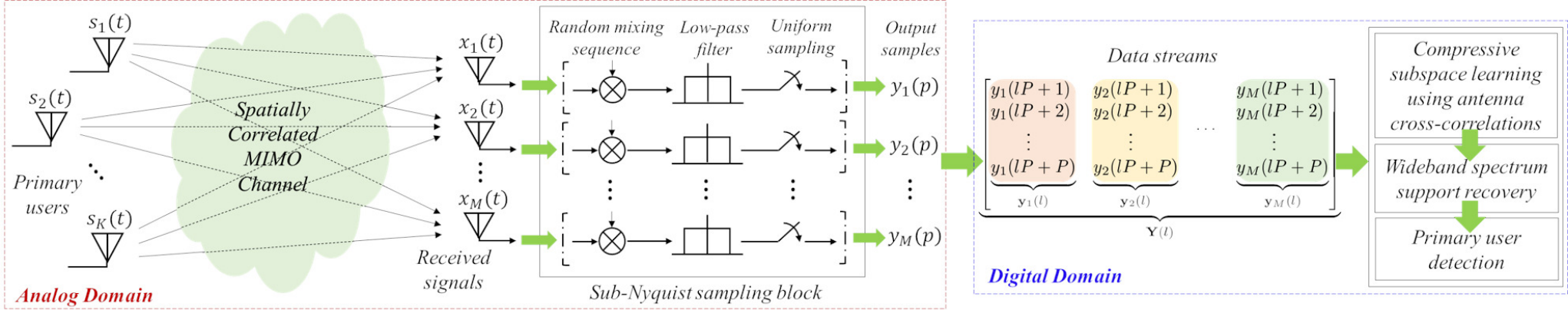
Consider an $M$-antenna CR that senses a wideband spectrum utilized by $K$ PUs. Each PU is equipped with one antenna and the PU signal, denoted as $s_{k}(t)$, is scattered in multiple paths to arrive at a receiving antenna, where such multiple scattered paths are equivalent to a single path with a channel gain $g_{mk}(t)$ as shown in the analog domain in Fig. 1. The channel gain matrix $\mathbf{G}\in\mathbb{C}^{M\times K}$ is defined and assumed to be fixed during a sensing period $T_{s}$. Without loss of generality, the received signal at the $m$th receiving antenna is denoted as $x_{m}(t)$, which is a sum of noise and $K$ faded PU signals. The noise, denoted as $n_{m}(t)$, is assumed a complex additive white Gaussian noise (AWGN) with zero mean and $\sigma^{2}_{m}$ variance, i.e., $n_{m}(t)\sim\mathcal{CN}(0,\sigma^{2}_{m})$. First, we denote $\bar{\mathbf{X}}=[\mathbf{x}_{1},\mathbf{x}_{2},\cdots,\mathbf{x}_{M}]^{T}\in\mathbb{C}^{M\times Q}$, $\bar{\mathbf{S}}=[\mathbf{s}_{1},\mathbf{s}_{2},\cdots,\mathbf{s}_{K}]^{T}\in\mathbb{C}^{K\times Q}$ and $\bar{\mathbf{N}}=[\bar{\mathbf{n}}_{1},\bar{\mathbf{n}}_{2},\cdots,\bar{\mathbf{n}}_{M}]^{T}\in\mathbb{C}^{M\times Q}$ as matrices with each column composed by $Q$ Nyquist samples of $x_{m}(t)$, $s_{k}(t)$ and $n_{m}(t)$, respectively. We then write the received sample matrix as

The PU signals $s_{k}(t)(1\leq k\leq K)$ are assumed to be independent with each other. The complex AWGN $n_{m}(t)(1\leq m\leq M)$ are assumed to be i.i.d. and also independent with the PU signals. The considered channels between the CR and PUs are denoted by a spatially correlated MIMO channel model described by the Kronecker model [37], whose channel gain matrix is given by

where $\mathbf{P}$ and $\mathbf{Q}$ are the transmitting and the receiving correlation matrices, respectively; $\mathbf{G}_{w}$ is a matrix constituted by i.i.d. complex Gaussian variables with zero mean and unit variance. The independence between any two PU signals makes the transmitting correlation matrix diagonal, i.e., $\mathbf{P}=diag\{\sigma_{1}^{2},\sigma_{2}^{2},\cdots,\sigma_{K}^{2}\}\in\mathbb{C}^{K\times K}$ with diagonal elements $\sigma_{k}^{2}(1\leq k\leq K)$ being transmit powers of PUs. To further characterize the receiving correlation matrix $\mathbf{Q}$, we define the correlation coefficient between the $m_{1}$th antenna and $m_{2}$th antenna as $\rho_{m_{1}m_{2}}\in\mathbb{C}(0\leq\left|\rho_{m_{1}m_{2}}\right|\leq 1)$. Then, we have $\mathbf{Q}=\left\{\rho_{m_{1}m_{2}}\right\}\in\mathbb{C}^{M\times M}(1\leq m_{1},m_{2}\leq M)$.

The received signals are passed to a multi-antenna sub-Nyquist sampling board to obtain the sub-sampled data streams. The received signal $x_{m}(t)$ of the $m$th antenna is then mixed with a random sequence, low-pass filtered, and uniformly sampled at $f_{m}$ to output the sub-samples $y_{m}(p)$ as shown in Fig. 1. The hardware configurations of all branches are set the same. The whole process of sub-Nyquist sampling can be represented by a measurement matrix $\mathbf{\Omega}\in\mathbb{C}^{P\times Q}$ with $P$ being the number of sub-samples and $P\ll Q$ [38]. Let $\mathbf{Y}=[\mathbf{y}_{1},\mathbf{y}_{2},\cdots,\mathbf{y}_{M}]\in\mathbb{C}^{P\times M}$ represent the sub-sample matrix of all antennas. Then, the input-output relation can be formulated as

For sub-Nyquist sampling based WBSS, the wideband spectrum is assumed to be sparse with a total sensed bandwidth limited to $W$ Hz and each bandwidth of a PU signal restricted to $B$ Hz. Each antenna receives a $W$ Hz wideband signal that is a linear superposition of $K$ different PU signals and an AWGN. Based on (3) and the frequency domain relation $\bar{\mathbf{X}}^{T}=\mathbf{\Psi}\mathbf{Z}+\bar{\mathbf{N}}^{T}$ with $\mathbf{Z}=[\mathbf{z}_{1},\mathbf{z}_{2},\cdots,\mathbf{z}_{M}]$ being the sparse Fourier coefficient matrix and $\mathbf{\Psi}$ being the discrete Fourier transform matrix, $\mathbf{Y}$ can be expressed in a sparse model as

with $\mathbf{A}\triangleq\mathbf{\Omega}\mathbf{\Psi}$ and $\mathbf{N}\triangleq\mathbf{\Omega}\bar{\mathbf{N}}^{T}$. Here the AWGN after sub-Nyquist sampling is still the AWGN yet with the larger noise power. The noise enhancement is induced by noise folding factor that is defined as the output-input noise power ratio of a sub-Nyquist sampling system [39]. We define the spectrum supports $\mathbb{S}=supp(\mathbf{Z})$ as the index set of disjoint narrowbands on which the Fourier coefficients of PU signals are lying. The spectrum supports $\mathbb{S}$ is unknown in prior due to the spectrum mobility of PUs. We aim to simultaneously detect the existing of PU signals and the corresponding spectrum support $\mathbb{S}$ from the sub-samples $\mathbf{Y}$.

Based on (1) and (3), $\mathbf{Y}$ can be reformulated as

As seen from (5), the sub-samples are influenced by both the wireless channel fading and the AWGN.

Aiming to obtain clean sub-samples from the noisy ones by using CSL algorithms, we expect to achieve a better WBSS performance [35]. Without prior information on the wireless channel and transmitted signals, we consider the blind recovery problem

with $\hat{\mathbf{Y}}$ being the constructed sub-samples and $\epsilon$ being the pre-specified bound for noise. It is noted that the constructed sub-samples can be either a matrix or a vector, which depends on the output of the CSL algorithm (corresponding to the vCSLACC algorithm and the mCSLSACC algorithm in Section III-A). Here, we use the matrix form, namely $\hat{\mathbf{Y}}$, without loss of generality. The matrix form denoting automatically reduces to the vector form if the output of the mCSLSACC algorithm is employed and the matrix $\mathbf{Z}$ correspondingly changes to the vector $\mathbf{z}$. To solve (6), we choose a greedy algorithm for the low computational complexity and simultaneous orthogonal matching pursuit (SOMP) [40] is properly used to achieve a feasible solution to the blind recovery problem in (6). We can alternatively integrate the constructed SCMs in (14) with the framework in [18, 19, 20] to realize the PSD recovery. However, as the emphasis of this paper lies in the influence analysis of the antenna and channel to the proposed CSL algorithms, we choose to adopt the spectrum recovery in (6) instead of the PSD recovery.

After the recovery stage, we use the energy detection method to make the final decision based on the recovered spectrum supports $\mathbb{S}$ and Fourier coefficients $\mathbf{Z}$. Specifically, for each $i\in\mathbb{S}$, the test statistics is given by $\mathcal{T}_{i}=\frac{1}{M}\sum_{m=1}^{M}|\mathbf{z}_{m}(i)|^{2}$. We define the probability of detection $p_{d}^{i}$ and the probability of false alarm $p_{f}^{i}$ for each spectrum support $i\in\mathbb{S}$, where $p_{d}^{i}=\mathbb{P}(\mathcal{T}_{i}>\gamma|\mathcal{H}_{1}^{i})$ and $p_{f}^{i}=\mathbb{P}(\mathcal{T}_{i}>\gamma|\mathcal{H}_{0}^{i})$ with $\mathcal{H}_{1}^{i}$ and $\mathcal{H}_{0}^{i}$ indicating the presence and absence of PUs on support $i$, $\gamma$ being a pre-defined non-negative threshold and $\mathbb{P}(\cdot)$ denoting the probability. Furthermore, let $\bar{\mathbb{S}}$ denote the complementary set of $\mathbb{S}$ such that $\mathbb{S}\cup\bar{\mathbb{S}}$ exactly consists of the whole index set of disjoint narrowbands. Then, the probabilities of detection and false alarm in terms of the spectrum support set $\mathbb{S}$ are defined as the averages of $p_{d}^{i}$ and $p_{f}^{i}$ over $\mathbb{S}$ and $\bar{\mathbb{S}}$, respectively, i.e.,

The entire process of the CSL based WBSS can be seen from the digital domain in Fig. 1.

We propose to exploit antenna cross-correlations and consider two different sub-sample operations ($\mathcal{A}_{m}$, $\mathcal{A}_{v}\in\mathscr{A}$) to realize the matrix and vector arrangements, respectively. Based on this idea, two CSL algorithms (i.e., mCSLSACC and vCSLACC) are proposed. We assume that in a sensing period each sub-sample data stream of an antenna is divided into $L$ segments with each segment $P$ sub-samples. In addition, we introduce an integer parameter $r(0\leq r\leq M-1)$ as the shift factor of antenna array to indicate the index shifting of a sub-array compared with another sub-array. Among all $M$ antennas, we select a consecutive sub-array indexed by $\mathbb{I}_{0}\triangleq\{i,i+1,\cdots,j\}(1\leq i\leq j\leq M-r)$ to generate the basic sub-sample group. Then another consecutive sub-array indexed by $\mathbb{I}_{r}\triangleq\{i+r,i+1+r,\cdots,j+r\}$ produces the shifted sub-sample group. When $r=0$, it is the antenna auto-correlation case, which is also considered for completeness. Without loss of generality, we consider the $l$th $(l\in[1,L])$ segment and give the following equations without including index $l$. The specific form by $\mathcal{A}_{m}$ shown in Fig. 2(a) is given by

where $\mathcal{A}_{m}(\mathbf{Y}_{\mathbb{I}_{0}}),\mathcal{A}_{m}(\mathbf{Y}_{\mathbb{I}_{r}})\in\mathbb{C}^{P\times(j-i+1)}$. For each $r$, we define $\mathbf{R}(\mathbf{Y},\mathcal{A}_{m},\mathbb{I}_{0},r)\triangleq\mathscr{E}\{\mathcal{A}_{m}(\mathbf{Y}_{\mathbb{I}_{0}})$ $\mathcal{A}_{m}^{H}(\mathbf{Y}_{\mathbb{I}_{r}})\}$ as an individual SCM. By collecting all individual cross-correlations to form a combined SCM $\mathbf{R}_{Y_{c}}\triangleq\sum_{r=1}^{i-1}\mathbf{R}(\mathbf{Y},\mathcal{A}_{m},\mathbb{I}_{0},-r)+\sum_{r=1}^{M-j}\mathbf{R}(\mathbf{Y},\mathcal{A}_{m},\mathbb{I}_{0},r)$ and learning the signal subspace from $\mathbf{R}_{Y_{c}}$, we derive the mCSLSACC. On the other hand, the vCSLACC is developed by learning signal subspace from a defined SCM $\mathbf{R}(\mathbf{Y},\mathcal{A}_{v},\mathbb{I}_{0},r)\triangleq\mathscr{E}\{\mathcal{A}_{v}(\mathbf{Y}_{\mathbb{I}_{0}})\mathcal{A}_{v}^{H}(\mathbf{Y}_{\mathbb{I}_{r}})\}$, in which the specific form by $\mathcal{A}_{v}$ shown in Fig. 2(b) is given by

where $\mathcal{A}_{v}(\mathbf{Y}_{\mathbb{I}_{0}}),\mathcal{A}_{v}(\mathbf{Y}_{\mathbb{I}_{r}})\in\mathbb{C}^{P(j-i+1)\times 1}$. The operation by $\mathcal{A}_{v}$ stacks sub-samples of each antenna into a vector in an increasing order from the $i$th ($i+r$th) to the $j$th ($j+r$th) antenna.

As stated in the solving process of problem (8), the signal subspace is obtained via an SVD, which is given by

where $\mathcal{A}\in\{\mathcal{A}_{m},\mathcal{A}_{v}\}$; $\mathbf{U}_{s}$ and $\mathbf{U}_{n}$ are matrices constituted by eigenvectors corresponding to signal and noise, respectively; $\mathbf{D}_{s}\triangleq diag\{\lambda_{1},\lambda_{2},\cdots,\lambda_{s}\}$ and $\mathbf{D}_{n}\triangleq diag\{\lambda_{s+1},\lambda_{s+2},\cdots,\lambda_{s+n}\}$ are diagonal matrices with singular values indicating signal and noise as their diagonal elements, respectively. The signal subspace $\mathbf{U}_{s}=[\mathbf{u}_{1},\mathbf{u}_{2},\cdots,\mathbf{u}_{s}]$ is determined by finding the $s$ largest singular values and the remaining $n$ singular values are used for noise subspace extraction, thereby resulting in a signal subspace projection $\mathbf{P}_{s}=\mathbf{U}_{s}\mathbf{U}_{s}^{H}$. We can construct the SCM and sub-samples via the obtained signal subspace as

where $\boldsymbol{\lambda}_{s}\triangleq[\lambda_{1},\lambda_{2},\cdots,\lambda_{s}]^{T}$. In practice, we estimate the SCM from finite sub-samples by averaging $L$ cross-correlations. The proposed algorithms are listed in Algorithm 1 and Algorithm 2, respectively.

It is worth noting that to learn subspaces from $\mathscr{E}\{\mathcal{A}(\mathbf{Y}_{\mathbb{I}_{0}})\mathcal{A}^{H}(\mathbf{Y}_{\mathbb{I}_{r}})\}$ is equivalent to learn the subspaces from $\mathscr{E}\{\mathcal{A}(\mathbf{Y}_{\mathbb{I}_{r}})\mathcal{A}^{H}(\mathbf{Y}_{\mathbb{I}_{0}})\}$ for $\mathcal{A}\in\{\mathcal{A}_{m},\mathcal{A}_{v}\}$. Therefore, we only take the former into consideration. In addition, we summarize the main differences of two proposed algorithms as follows:

• •

  For all different values of $r$, the mCSLSACC corresponds to the case of only one input-output vector pair for its decomposed SCM being a combined result over $r$, while the vCSLACC includes $r$ input-output vector pairs. In addition, the number of dominant singular values (i.e., $s$) are different for both algorithms.

• •

  The basic SCM used to constitute $\mathbf{R}_{Y_{c}}$ in the mCSLSACC is a sum of individual $\mathscr{E}\{\mathbf{y}_{m}\mathbf{y}_{m+r}^{H}\}$ $(i\leq m\leq j)$ with equal weights over $j-i+1$ antennas. Therefore, the signal subspace is obtained as a superposition result and its bases expands on the time dimension. Nevertheless, the SCM in the vCSLACC is constituted by sub-matrices $\mathscr{E}\{\mathbf{y}_{m_{1}}\mathbf{y}_{m_{2}}^{H}\}(i\leq m_{1}\leq j,i+r\leq m_{2}\leq j+r)$, leading to a spatial-temporal joint decomposition.

To establish the SCM of the mCSLACC, we arrange the corresponding Nyquist samples $\mathbf{s}_{k}=[s_{k}(lQ+1),s_{k}(lQ+2),\cdots,s_{k}(lQ+Q)]^{T}$ and $\mathbf{c}_{m}=[c_{m}(lQ+1),c_{m}(lQ+2),\cdots,c_{m}(lQ+Q)]^{T},1\leq m\leq M,c\in\{x,n\}$ into matrices as

where $\mathbf{c}\in\{\mathbf{x},\mathbf{n}\}$, $\mathbf{C}\in\{\mathbf{X},\mathbf{N}\}$. Defining $\mathbf{C}_{\mathbb{I}_{0}}\triangleq[\mathbf{C}]_{:,i:j}$, $\mathbf{C}_{\mathbb{I}_{r}}\triangleq[\mathbf{C}]_{:,(i+r):(j+r)}$ and following (5), we get

where $\mathbf{G}_{\mathbb{I}_{0}}^{T}\triangleq[\mathbf{G}^{T}]_{:,i:j}$ and $\mathbf{G}_{\mathbb{I}_{r}}^{T}\triangleq[\mathbf{G}^{T}]_{:,(i+r):(j+r)}$. Then, $\mathbf{R}(\mathbf{Y},\mathcal{A}_{m},\mathbb{I}_{0},r)$ can be further given by

where $\mathbf{g}_{k}$ is denoted as the $k$th column of $\mathbf{G}$ with $[\mathbf{g}_{k}^{T}]_{\mathbb{I}_{0}}\triangleq[\mathbf{g}_{k}^{T}]_{i:j}$ and $[\mathbf{g}_{k}^{T}]_{\mathbb{I}_{r}}\triangleq[\mathbf{g}_{k}^{T}]_{(i+r):(j+r)}$; $\mathbf{R}_{s_{k}}\triangleq\mathscr{E}\left\{\mathbf{s}_{k}\mathbf{s}_{k}^{H}\right\}$ and $\mathbf{R}(\mathbf{N},\mathcal{A}_{m},\mathbb{I}_{0},r)\triangleq\mathscr{E}\{\mathcal{A}_{m}(\mathbf{N}_{\mathbb{I}_{0}})\mathcal{A}_{m}^{H}(\mathbf{N}_{\mathbb{I}_{r}})\}$. (18) is derived by following the fact that $\mathscr{E}\left\{\mathbf{s}_{k_{1}}\mathbf{s}_{k_{2}}^{H}\right\}=\mathbf{0}$ when $k_{1}\neq k_{2}$. For the noise term $\mathbf{R}(\mathbf{N},\mathcal{A}_{m},\mathbb{I}_{0},r)$, discussions are listed as follows:

• •

  At $r=0$, the noise term comes from an auto-correlation of $\mathbf{N}_{\mathbb{I}_{0}}$, thereby leading to the only use of antenna auto-correlations. It, thus, becomes a diagonal matrix $\sigma_{N_{\mathbb{I}_{0}}}^{2}\mathbf{I}_{P}$ with $\sigma_{N_{\mathbb{I}_{0}}}^{2}\triangleq\sum_{m\in\mathbb{I}_{0}}\alpha_{m}\sigma_{m}^{2}$ and $\alpha_{m}$ being the noise folding factor. This condition leads to a noise corruption to $\mathbf{R}(\mathbf{Y},\mathcal{A}_{m},\mathbb{I}_{0},r)$.

• •

  When $r\neq 0$, the noise term is obtained based on the cross-correlation between $\mathbf{N}_{\mathbb{I}_{0}}$ and $\mathbf{N}_{\mathbb{I}_{r}}$, allowing the exploitation of antenna cross-correlations without being faced with the noise corruption at $r=0$. This reveals that $\mathbf{R}(\mathbf{Y},\mathcal{A}_{m},\mathbb{I}_{0},r)$ is not interfered by noise for $r\neq 0$.

Throughout the above discussions, we can exploit the second condition to improve the signal subspace learning in the low SNR scenario.

To establish the SCM relation between the basic mCSLACC and traditional CSL algorithms for further analysis, both SCMs in statistical sense w.r.t. the wireless fading channel are investigated. Following the Kronecker model in (2), we obtain $\mathbf{g}_{k}=\sigma_{k}\mathbf{Q}^{\frac{1}{2}}\bar{\mathbf{g}}_{k}$, where $\sigma_{k}$ is the $k$th diagonal element of $\mathbf{P}^{\frac{1}{2}}$ and $\bar{\mathbf{g}}_{k}$ is the $k$th column of matrix $\mathbf{G}_{w}$ whose elements follow the Rayleigh distribution with zero mean and unit variance. Let $\mathbf{q}_{m}(1\leq m\leq M)$ be columns of $\mathbf{Q}^{\frac{1}{2}}$. Then we get

where $\mathscr{E}\left\{\bar{g}_{m_{1}k}\bar{g}_{m_{2}k}^{*}\right\}=0,\forall m_{1}\neq m_{2}$ and $\mathscr{E}\left\{\left|\bar{g}_{mk}\right|^{2}\right\}=1,\forall m$ are used for the derivation. The last equality in (19) follows the Hermitian structure of $\mathbf{Q}^{\frac{1}{2}}$.

Taking expectation to both sides of (18) and using (19), we obtain

where $\bar{\mathbf{R}}(\mathbf{Y},\mathcal{A}_{m},\mathbb{I}_{0},r)\triangleq\mathscr{E}_{\mathbf{g}_{k}}\left\{\mathbf{R}(\mathbf{Y},\mathcal{A}_{m},\mathbb{I}_{0},r)\right\}$ represents the SCM in statistical sense w.r.t. the wireless fading channel and $\bar{\mathbf{R}}_{sa}\triangleq\mathbf{\Omega}\sum_{k=1}^{K}{\sigma_{k}^{2}}\mathbf{R}_{s_{k}}\mathbf{\Omega}^{H}$. The matrix $\bar{\mathbf{R}}_{sa}$ coincides with the SCM in statistical sense of traditional CSL algorithms considering the MIMO channel without spatial correlations (i.e., by setting $\mathbf{g}_{k}={\sigma_{k}}\mathbf{I}_{M}\bar{\mathbf{g}}_{k}$). It is noted from (20) that the mCSLACC introducs $G\triangleq\sum\nolimits_{u\in\mathbb{I}_{0}}{\mathbf{q}_{u}^{H}\mathbf{q}_{u+r}}$ over traditional CSL algorithms in statistical sense in terms of SCM.

Based on the derived relation in (20), we next show how the spatially correlated MIMO channel and the shift factor of antenna sub-arrays influence the performance of the mCSLACC by comparing it with traditional CSL algorithms. The comparison is based on a relation between singular values of two SCMs. Such a singular value relation helps us understand the amplification introduced by the mCSLACC, where the large amplification on singular values allows an accurate discrimination from noise than traditional CSL algorithms.

We define singular value matrices $\mathbf{D}(\mathbf{Y},\mathcal{A}_{m},\mathbb{I}_{0},r)\triangleq sv\left(\bar{\mathbf{R}}(\mathbf{Y},\mathcal{A}_{m},\mathbb{I}_{0},r)\right)$ and $\mathbf{D}_{sa}\triangleq sv\left(\bar{\mathbf{R}}_{sa}\right)$, allowing the derivation of the singular value relation in (20) as

We note that the singular values in $\mathbf{D}(\mathbf{Y},\mathcal{A}_{m},\mathbb{I}_{0},r)$ are amplified results of the singular values in $\mathbf{D}_{sa}$ by an amplification factor $|G|\triangleq\left|\sum\nolimits_{u\in\mathbb{I}_{0}}{\mathbf{q}_{u}^{H}\mathbf{q}_{u+r}}\right|$.

In order to provide more insights on the derived amplification factor, the exponential correlation model is used to describe the receiving correlation matrix, whose specific form is given by

where $\rho$ is a coefficient (known as correlation coefficient) characterizing the correlation between adjacent antennas. This model shows that the correlations are the same for equally spaced antennas and are exponentially decayed for increasingly spaced antennas. With such an exponential correlation model and the equation $\mathbf{Q}^{\frac{1}{2}}(\mathbf{Q}^{\frac{1}{2}})^{H}=\mathbf{Q}$, we obtain the correlation between the $m_{1}$th and $m_{2}$th columns of $\mathbf{Q}^{\frac{1}{2}}$ as

Accordingly, the amplification factor $|G|$ is obtained based on (23) as

As in (24), the $|G|$ reduces to $j-i+1$ at $r=0$, which is equivalent to traditional CSL algorithms considering spatially uncorrelated MIMO channel. Dividing the noise term $\sigma_{N_{\mathbb{I}_{0}}}^{2}\mathbf{I}_{P}$ by $j-i+1$, the mCSLACC can be considered as an antenna averaging scheme, which makes the mCSLACC robust against noise. When $r\neq 0$, the $|G|$ reduces by the correlation coefficient $|\rho|$ with an increasing $r$, which reveals that the amplification effect by antenna cross-correlations becomes weak with the increasing of antenna distances. However, the superiority of mCSLACC at $r\neq 0$ over that at $r=0$ is attributed to the lack of noise corruption. Moreover, in the case of $r\neq 0$, a large correlation coefficient indeed promotes an improved amplification effect, while in the case of $r=0$, the fact $|\rho|^{0}=1$ shows that $|G|$ does not change with varying correlation coefficients. As expected, both cases are influenced by the number of deployed antennas $j-i+1$, where both of their performances improve with the increasing $j-i+1$.

As previously discussed, we can tell from (21) that, for each $r\neq 0$, the SCM of mCSLACC enjoys noise-free property and introduces a $|G|$ over the singular values of SCM in traditional CSL algorithms. Since $|G|$ exponentially decayed, taking advantage of all noise-free amplifications is necessary. To this end, we propose the mCSLSACC. By summing up individual SCMs $\mathbf{R}(\mathbf{Y},\mathcal{A}_{m},\mathbb{I}_{0},r)$ $(1\leq r\leq M-j)$ over $r$ for a given sub-array indexed by $\mathbb{I}_{0}$, we obtain the statistical relation based on (20) between the combined SCM $\mathbf{R}_{Y_{c}}$ and the SCM of traditional CSL algorithms as

Then, based on (25), the singular value relation is given by

where $\mathbf{D}_{Y_{c}}\triangleq sv\left(\bar{\mathbf{R}}_{Y_{c}}\right)$. With the exponential correlation model, the following theorem gives the amplification factor by the mCSLSACC.

Given a fixed $M$, $|G|$ in (27) does not always increase with the increasing $j-i+1$. The maximum of $|G|$ exists, depending on both $|\rho|$ and $j-i+1$. Accordingly, Theorem 1 can be used as a criterion to determine the optimal $j-i+1$ that maximizes $|G|$.

Discussion 1: Theorem 1 bridges a connection between the singular value gain and the spatial correlation as well as the number of deployed antennas, providing us a convenient way to analyze how such factors influence the singular values in statistical sense. As the recovery stage retains for the WBSS, the singular values of CSL algorithms should be discriminated from noise for signal subspace extraction. Considering that the large singular value makes the discrimination accurate, one can use the amplification factor as a guide to design an MIMO system that satisfies the discrimination standard of singular values. For a given SNR that enables traditional CSL algorithms, we can design the spatial correlation and the number of deployed antennas to meet the SNR that enables the discrimination of singular values. Additionally, given a fixed number of total antennas, the theoretical result provides a criterion to determine the optimal number of deployed antennas when one uses the proposed mCSLSACC algorithm.

In the vCSLACC, the Nyquist samples and sub-samples are reorganized by operator $\mathcal{A}_{v}$, which stacks the columns of matrices into vectors. More specifically, defining vectors $\mathbf{n}_{\mathbb{I}_{0}}\triangleq vec(\mathbf{N}_{\mathbb{I}_{0}})$, $\mathbf{n}_{\mathbb{I}_{r}}\triangleq vec\left(\mathbf{N}_{\mathbb{I}_{r}}\right)$ and $\mathbf{s}\triangleq vec(\mathbf{S})$, and vectorizing both sides of (16) and (17), we obtain

The SCM $\mathbf{R}(\mathbf{Y},\mathcal{A}_{v},\mathbb{I}_{0},r)$ is thus derived based on (28) and (29) as

where $\mathbf{R}_{\mathbf{s}}\triangleq\mathscr{E}\left\{\mathbf{s}\mathbf{s}^{H}\right\}$ is a block diagonal matrix, with $\mathbf{R}_{s_{k}}(1\leq k\leq K)$ being the diagonal blocks. The second equality of (30) follows the block diagonal structure of $\mathbf{R}_{\mathbf{s}}$. We discuss different cases of the noise term $\mathbf{R}(\mathbf{N},\mathcal{A}_{v},\mathbb{I}_{0},r)$ as follows:

• •

  When $0\leq r\leq j-i$, the noise term $\mathbf{R}(\mathbf{N},\mathcal{A}_{v},\mathbb{I}_{0},r)$ exists as a block off-diagonal (diagonal when $r=0$) matrix of dimension $(j-i+1)P$, whose off-diagonal blocks are given by $\mathbf{\Pi}_{m}\triangleq diag\{\alpha_{m}\sigma^{2}_{m},\cdots,\alpha_{m}\sigma^{2}_{m}\}$ $\in\mathbb{C}^{P\times 1}$ $(1\leq m\leq j-i+1-r)$. The SCM $\mathbf{R}(\mathbf{Y},\mathcal{A}_{v},\mathbb{I}_{0},r)$ is therefore corrupted by noise.

• •

  The noise term $\mathbf{R}(\mathbf{N},\mathcal{A}_{v},\mathbb{I}_{0},r)$ disappears when $j-i<r\leq M-j$ and the SCM $\mathbf{R}(\mathbf{Y},\mathcal{A}_{v},\mathbb{I}_{0},r)$ is therefore not corrupted by noise. As a result, the vCSLACC can be used to improve the performance of signal subspace learning in low SNR scenarios.

In order to establish the SCM relation between the proposed vCSLACC and traditional CSL algorithms for further analysis, we similarly investigate the SCMs in statistical sense w.r.t. the wireless fading channel as in Section IV-A. First of all, we derive $\mathscr{E}\left\{[\mathbf{g}_{k}]_{\mathbb{I}_{0}}[\mathbf{g}_{k}^{H}]_{\mathbb{I}_{r}}\right\}$ as

where $\mathbf{T}_{i,j,r}$ is a sub-matrix constituted by rows of $\mathbf{Q}$ indexed from $i$ to $j$ and columns of $\mathbf{Q}$ indexed from $i+r$ to $j+r$. Plugging (31) into the expectation of (30), we then get

References

- [1] FCC, “Spectrum task force report: Federal communications commission,” Tech. Rep. ET Docket no. 02-135, Nov. 2002.
- [2] M. Mchenry, “NSF spectrum occupancy measurements project summary,” shared spectrum co., Tech. Rep., Aug. 2005.
- [3] Y. Chen and H. S. Oh, “A survey of measurement-based spectrum occupancy modeling for cognitive radios,” IEEE Commun. Surveys Tuts., vol. 18, no. 1, pp. 848–859, Firstquarter 2016.
- [4] S. Haykin, “Cognitive radio: Brain-empowered wireless communications,” IEEE J. Sel. Areas Commun., vol. 23, no. 2, pp. 201–220, Feb. 2005.
- [5] T. Yucek and H. Arslan, “A survey of spectrum sensing algorithms for cognitive radio applications,” IEEE Commun. Surveys Tuts., vol. 11, no. 1, pp. 116–130, Firstquarter 2009.
- [6] M. Zheng, W. Liang, H. Yu, and M. Song, “SMCSS: A quick and reliable cooperative spectrum sensing scheme for cognitive industrial wireless networks,” IEEE Access, vol. 4, pp. 9308–9319, 2016.
- [7] M. Zheng, L. Chen, W. Liang, H. Yu, and J. Wu, “Energy-efficiency maximization for cooperative spectrum sensing in cognitive sensor networks,” IEEE Trans. Green Commun. Netw., vol. 1, no. 1, pp. 29–39, Mar. 2017.
- [8] G. Hattab and M. Ibnkahla, “Multiband spectrum access: Great promises for future cognitive radio networks,” Proc. IEEE, vol. 102, no. 3, pp. 282–306, Mar. 2014.
- [9] A. Ali and W. Hamouda, “Advances on spectrum sensing for cognitive radio networks: Theory and applications,” IEEE Commun. Surveys Tuts., vol. 19, no. 2, pp. 1277–1304, Secondquarter 2017.
- [10] B. Hamdaoui, B. Khalfi, and M. Guizani, “Compressed wideband spectrum sensing: Concept, challenges, and enablers,” IEEE Commun. Mag., vol. 56, no. 4, pp. 136–141, Apr. 2018.
- [11] Z. Qin, J. Fan, Y. Liu, Y. Gao, and G. Y. Li, “Sparse representation for wireless communications: A compressive sensing approach,” IEEE Signal Process. Mag., vol. 35, no. 3, pp. 40–58, May 2018.
- [12] E. J. Candes, J. Romberg, and T. Tao, “Robust uncertainty principles: Exact signal reconstruction from highly incomplete frequency information,” IEEE Trans. Inf. Theory, vol. 52, no. 2, pp. 489–509, Feb. 2006.
- [13] M. Mishali and Y. C. Eldar, “Sub-nyquist sampling,” IEEE Signal Process. Mag., vol. 28, no. 6, pp. 98–124, Nov. 2011.
- [14] B. Khalfi, B. Hamdaoui, M. Guizani, and N. Zorba, “Efficient spectrum availability information recovery for wideband DSA networks: A weighted compressive sampling approach,” IEEE Trans. Wireless Commun., vol. 17, no. 4, pp. 2162–2172, Apr. 2018.
- [15] P. Qi, Z. Li, H. Li, and T. Xiong, “Blind sub-Nyquist spectrum sensing with modulated wideband converter,” IEEE Trans. Veh. Technol., vol. 67, no. 5, pp. 4278–4288, May 2018.
- [16] X. Zhang, Y. Ma, Y. Gao, and W. Zhang, “Autonomous compressive-sensing-augmented spectrum sensing,” IEEE Trans. Veh. Technol., vol. 67, no. 8, pp. 6970–6980, Aug. 2018.
- [17] F. Wang, J. Fang, H. Duan, and H. Li, “Phased-array-based sub-Nyquist sampling for joint wideband spectrum sensing and direction-of-arrival estimation,” IEEE Trans. Signal Process., vol. 66, no. 23, pp. 6110–6123, Dec. 2018.
- [18] D. D. Ariananda and G. Leus, “Compressive wideband power spectrum estimation,” IEEE Trans. Signal Process., vol. 60, no. 9, pp. 4775–4789, Sep. 2012.
- [19] D. Cohen and Y. C. Eldar, “Sub-Nyquist sampling for power spectrum sensing in cognitive radios: A unified approach,” IEEE Trans. Signal Process., vol. 62, no. 15, pp. 3897–3910, Aug. 2014.
- [20] D. Romero, D. D. Ariananda, Z. Tian, and G. Leus, “Compressive covariance sensing: Structure-based compressive sensing beyond sparsity,” IEEE Signal Process. Mag., vol. 33, no. 1, pp. 78–93, Jan. 2016.
- [21] H. Sun, A. Nallanathan, C. X. Wang, and Y. Chen, “Wideband spectrum sensing for cognitive radio networks: A survey,” IEEE Wireless Commun., vol. 20, no. 2, pp. 74–81, Apr. 2013.
- [22] A. Taherpour, M. Nasiri-Kenari, and S. Gazor, “Multiple antenna spectrum sensing in cognitive radios,” IEEE Trans. Wireless Commun., vol. 9, no. 2, pp. 814–823, Feb. 2010.
- [23] X. Yang, Q. Cui, R. Yang, X. Tao, and X. Guo, “Multi-antenna compressed wideband spectrum sensing for cognitive radio,” in Proc. IEEE Wireless Commun. and Netw. Conf., Mar. 2011, pp. 1903–1908.
- [24] S. S. Ioushua, O. Yair, D. Cohen, and Y. C. Eldar, “CaSCADE: Compressed carrier and DOA estimation,” IEEE Trans. Signal Process., vol. 65, no. 10, pp. 2645–2658, May 2017.
- [25] C. Masouros, M. Sellathurai, and T. Ratnarajah, “Large-scale MIMO transmitters in fixed physical spaces: The effect of transmit correlation and mutual coupling,” IEEE Trans. Commun., vol. 61, no. 7, pp. 2794–2804, July 2013.
- [26] T. Gong, Z. Yang, and M. Zheng, “Compressive subspace learning based wideband spectrum sensing for multiantenna cognitive radio,” IEEE Trans. Veh. Technol., vol. 68, no. 7, pp. 6636–6648, July 2019.
- [27] M. S. Oude Alink, A. B. J. Kokkeler, E. A. M. Klumperink, G. J. M. Smit, and B. Nauta, “Lowering the SNR wall for energy detection using cross-correlation,” IEEE Trans. Veh. Technol., vol. 60, no. 8, pp. 3748–3757, Oct. 2011.
- [28] M. Kitsunezuka and K. S. J. Pister, “Cross-correlation-based, phase-domain spectrum sensing with low-cost software-defined radio receivers,” IEEE Trans. Signal Process., vol. 63, no. 8, pp. 2033–2048, Apr. 2015.
- [29] J. C. Merritt and J. D. Chisum, “High-speed cross-correlation for spectrum sensing and direction finding of time-varying signals,” IEEE Sensors J., vol. 18, no. 15, pp. 6161–6168, Aug. 2018.
- [30] Y. Zeng and Y. C. Liang, “Eigenvalue-based spectrum sensing algorithms for cognitive radio,” IEEE Trans. Commun., vol. 57, no. 6, pp. 1784–1793, June 2009.
- [31] Z. Li, D. Wang, P. Qi, and B. Hao, “Maximum-eigenvalue-based sensing and power recognition for multiantenna cognitive radio system,” IEEE Trans. Veh. Technol., vol. 65, no. 10, pp. 8218–8229, Oct. 2016.
- [32] C. Liu, H. Li, J. Wang, and M. Jin, “Optimal eigenvalue weighting detection for multi-antenna cognitive radio networks,” IEEE Trans. Wireless Commun., vol. 16, no. 4, pp. 2083–2096, Apr. 2017.
- [33] K. Bouallegue, I. Dayoub, M. Gharbi, and K. Hassan, “Blind spectrum sensing using extreme eigenvalues for cognitive radio networks,” IEEE Commun. Lett., vol. 22, no. 7, pp. 1386–1389, July 2018.
- [34] M. Jin, Q. Guo, Y. Li, J. Xi, and D. Huang, “Spectrum sensing using multiple large eigenvalues and its performance analysis,” IEEE Internet Things J., vol. 6, no. 1, pp. 776–789, Feb. 2019.
- [35] Y. Ma, Y. Gao, Y. C. Liang, and S. Cui, “Reliable and efficient sub-Nyquist wideband spectrum sensing in cooperative cognitive radio networks,” IEEE J. Sel. Areas Commun., vol. 34, no. 10, pp. 2750–2762, Oct. 2016.
- [36] X. Zhang, Y. Ma, H. Qi, Y. Gao, Z. Xie, M. Zhang, X. Wang, G. Wei, and Z. Li, “Distributed compressive sensing augmented wideband spectrum sharing for cognitive IoT,” IEEE Internet Things J., vol. 5, no. 4, pp. 3234–3245, Aug. 2018.
- [37] N. Costa and S. Haykin, Multiple-Input, Multiple-Output Channel Models: Theory and Practice. John Wiley & Sons, Inc., 2010.
- [38] J. A. Tropp, J. N. Laska, M. F. Duarte, J. K. Romberg, and R. G. Baraniuk, “Beyond Nyquist: Efficient sampling of sparse bandlimited signals,” IEEE Trans. Inf. Theory, vol. 56, no. 1, pp. 520–544, Jan. 2010.
- [39] T. Gong, Z. Liu, C. Xie, and Z. Yang, “Property investigation on the additive white Gaussian noise after sub-Nyquist sampling,” IEEE Access, vol. 7, pp. 122 820–122 826, 2019.
- [40] J. A. Tropp, A. C. Gilbert, and M. J. Strauss, “Simultaneous sparse approximation via greedy pursuit,” in Proc. IEEE Int. Conf. Acoust., Speech, Signal Process., Mar. 2005, pp. 721–724.
- [41] J. Choi and D. J. Love, “Bounds on eigenvalues of a spatial correlation matrix,” IEEE Commun. Lett., vol. 18, no. 8, pp. 1391–1394, Aug. 2014.
- [42] H. Lim, Y. Jang, and D. Yoon, “Bounds for eigenvalues of spatial correlation matrices with the exponential model in MIMO systems,” IEEE Trans. Wireless Commun., vol. 16, no. 2, pp. 1196–1204, Feb. 2017.
- [43] T. Gong, G. Yang, K. Mu, C. Zhao, and Z. Yang, “An improved upper bound on the maximum eigenvalue of exponential model based spatial correlation matrices in massive MIMO systems,” in Proc. IEEE Int. Conf. Commun. Technol., Oct. 2019, pp. 638–642.
- [44] S. Park, A. Alkhateeb, and R. W. Heath, “Dynamic subarrays for hybrid precoding in wideband mmwave MIMO systems,” IEEE Trans. Wireless Commun., vol. 16, no. 5, pp. 2907–2920, May 2017.
- [45] G. A. F. Seber, A Matrix Handbook for Statisticians. John Wiley & Sons, Inc., 2007.