Unsupervised Deep Learning for Optimizing Wireless Systems with Instantaneous and Statistic ConstraintsThis paper has been presented in part at the IEEE Global Communications Conference 2019 [1] and in part at the IEEE International Symposium on Personal, Indoor and Mobile Radio Communications 2019 [2].C. Sun and C. Yang are with the School of Electronics and Information Engineering, Beihang University, Beijing 100191, China (email:{sunchengjian,cyyang}@buaa.edu.cn).C. She is with the School of Electrical and Information Engineering, University of Sydney, Sydney, NSW 2006, Australia (e-mail: shechangyang@gmail.com).

The theory of calculus of variations in [6] indicates that the optimal solution of problem (4) should satisfy the following conditions,

From the definition of the Lagrangian, (5) can be derived as follows,

which is the simplified form of the Eular-Lagrange equation defined in [6].

These conditions are the first-order necessary conditions to achieve the optimality of functional optimization problems, like the KKT conditions of variable optimization problems [17]. However, the condition in (7) is an integral equation, which comes from the statistic constraints. This makes solving functional optimization problems rather challenging. In particular, even if the closed-form expression of $\bm{x}(\bm{\theta})$ can be obtained from (5), (6), (8), (4a) and (4b), the closed-form expressions of Lagrange multiplier for the statistic constraints $\lambda_{j},j=I+1,...,I+J$ are hard to derive since integral equations are in general difficult to solve. For example, the optimal solution of problem (3) is the well-known “water-filling” policy, where the water level satisfying (7) and (4b) does not have closed-form expression and has to be obtained from binary search in [16]. On the other hand, if the closed-form expression of $\bm{x}(\bm{\theta})$ cannot be obtained, one has to employ the FEM with extremely high complexity for finding the numerical result of the integration in (7).

In what follows, we resort to unsupervised deep learning to solve problem (4).

To deal with the constraints of a problem, one can solve its primal-dual problem. In particular, if problem (4) is convex and the Slater’s condition holds, then it is equivalent to the following problem [17, 6],

The Slater’s condition generally holds in optimization problems with continues variables. However, the convexity does not hold in many cases. If the problem is non-convex, a local optimal solution of problem (4) can be obtained by solving problem (10) [18].

To find the solution with unsupervised deep learning, we approximate the two functions in $L$, $\bm{x}(\bm{\theta})$ and $\bm{{v}}(\bm{\theta})\triangleq[{{v}}_{1}(\bm{\theta}),...,{{v}}_{I}(\bm{\theta})]^{\rm T}$, by two DNNs denoted as $\mathcal{N}_{x}(\bm{\theta};\bm{\omega}_{x})$ and $\mathcal{N}_{v}(\bm{\theta};\bm{\omega}_{v})$ respectively with model parameters $\bm{\omega}_{x}$ and $\bm{\omega}_{v}$. According to the Universal Approximation Theory, a deterministic continuous function defined over a compact set can be approximated by a DNN, and the approximation can be arbitrarily accurate [19]. By replacing $\bm{x}(\bm{\theta})$ and $\bm{{v}}(\bm{\theta})$ with $\hat{\bm{x}}(\bm{\theta})\!\triangleq\!\mathcal{N}_{x}(\bm{\theta};\bm{\omega}_{x})$ and $\hat{\bm{{v}}}(\bm{\theta})\!\triangleq\!\mathcal{N}_{v}(\bm{\theta};\bm{\omega}_{v})$, problem (10) can be re-written as,

Then, the primal-dual method can be used to update primal variables $\bm{\omega}_{x}$, dual variables ${\bm{\omega}}_{v}$, and the Lagrange multiplier for statistical constraint ${\lambda}_{j}$ iteratively to find a solution of problem (11). At the $t$th iteration, these variables can be updated by the stochastic gradient descent (SGD) method and the stochastic gradient ascent (SGA) method as

where ${\left(x\right)}^{+}\!\triangleq\!\max\!{\left\{x,0\right\}}$ ensures ${{{\lambda}}}_{j}^{(t+1)}>0$, $\phi_{\omega_{x}}(t)$, $\phi_{\omega_{{v}}}(t)$ and $\phi_{{{\lambda}}_{j}}(t)$ are the learning rates for updating $\bm{\omega}_{x}$, ${\bm{\omega}}_{v}$ and ${\lambda}_{j}$, and ${\nabla_{\omega_{x}}}\hat{L}^{(t)}$ and ${\nabla_{\omega_{v}}}\hat{L}{{}^{(}t)}$ are the gradients of $\hat{L}$ w.r.t. ${\omega_{x}}$ and ${\omega_{v}}$, respectively.¹¹ 1 The gradient of a scalar $x$ w.r.t. to a vector ${\bm{y}}_{N_{y}\times 1}$ is defined as $\nabla_{{\bm{y}}}x\triangleq[{\partial{x}}/{\partial{y_{1}}},...,{\partial x}/{\partial y_{N_{y}}}]^{\rm T}$ and the gradient of a vector $\bm{x}_{N_{x}\times 1}$ w.r.t. to a vector ${\bm{y}}_{N_{y}\times 1}$ is defined as $\nabla_{{\bm{y}}}\bm{x}\triangleq[\nabla_{{\bm{y}}}{x_{1}},...,\nabla_{{\bm{y}}}{x_{N_{x}}}]$. The method to compute the gradient and derivative is provided in Appendix B.

To guarantee $\hat{{v}}_{i}(\bm{\theta})\geq{0},\forall{\bm{\theta}\in\mathcal{D}_{\theta}}$, we need to choose a proper activation function in the output layer of $\mathcal{N}_{v}(\bm{\theta};\bm{\omega}_{v})$, e.g., $\texttt{ReLU}(x)\triangleq\max(x,0)$ or $\texttt{SoftPlus}(x)\triangleq\ln[1+\exp(x)]$ [20, 21].

The DNNs are trained by optimizing $\bm{\omega}_{x}$, $\bm{\omega}_{v}$, ${\lambda}_{j}$, $j=I+1,...,I+J$ respectively with the SGD and SGA methods. As shown in [9], the primal-dual method converges at least to a local optimal solution of the primal-dual problem of the original problem. A local optimal solution is either at a stationary point of $\hat{L}$ or on the boundary of the feasible region. Thus, the following properties hold for the obtained solutions: $\nabla_{\bm{\omega}_{x}}\hat{L}=\bm{0}$, $\nabla_{\bm{\omega}_{v}}\hat{L}=\bm{0}$ (or $\hat{{v}_{i}}(\bm{\theta})=0$) and ${\partial\hat{L}}/{\partial{\lambda}_{j}}=0$ (or ${\lambda}_{j}=0$), $j=I+1,...,I+J$. These properties implicitly serve as the “supervised signal” of the DNNs. Since the DNNs are trained without labels, it belongs to unsupervised learning.

Consider a DL orthogonal frequency division multiple access system, where a BS with $N_{\mathrm{t}}$ antennas serves $K$ single-antenna users. The maximal transmit power and the total bandwidth of the BS are denoted by $P_{\mathrm{max}}$ and $W_{\max}$, respectively.

The packets for each user arrive at the buffer of the BS randomly. The inter-arrival time between packets could be shorter than the service time of each packet. Therefore, the packets may wait in the buffer of the BS. We consider a queueing model that the packets for different users wait in different queues and are served according to a first-come-first-serve order.

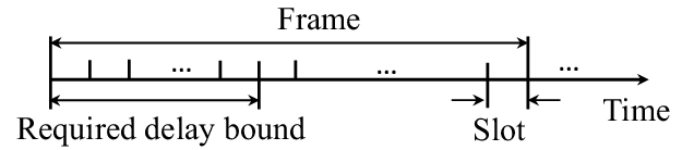
Time is discretized into slots, each with duration $T_{\mathrm{s}}$. The duration for DL data transmission in one time slot is $\tau<T_{\mathrm{s}}$. Since the E2E delay requirement in URLLC is typically shorter than the coherence time of small-scale channel, the channel is quasi-static and time diversity cannot be exploited. To improve the transmission reliability within the delay bound, we consider frequency hopping, where each user is assigned with different subchannels in adjacent slots. When the frequency interval between adjacent subchannels is larger than the coherence bandwidth, the small-scale channel gains of a user among slots are mutual independent. Since the packet size $u$ in URLLC is typically small (e.g., $20$ bytes or $32$ bytes [22]), the bandwidth required for transmitting each packet is less than the channel coherence bandwidth. Therefore, the small-scale channel is flat fading.

As shown in [16], the large-scale channel gain of a user varies when its moving distance is comparable to the decorrelation distance of shadowing, i.e., $50\sim 100$ m. Thus, the coherence time of the large-scale channel gain is around a few seconds, much longer than the delay bound $D_{\mathrm{max}}$ and the slot duration $T_{\mathrm{s}}$ (e.g., in 5G New Radio, $T_{\mathrm{s}}$ can be much shorter than $1$ ms [3]). We assume that large-scale channel gains stay constant in each frame that consists of $N_{\rm f}$ time slots, and may vary in different frames. The relations among the timescales of the frames, slots, and the required delay bound are illustrated in Fig. 1.

In URLLC, the blocklength of channel coding is short due to the short transmission duration, and hence the impact of decoding errors on reliability cannot be ignored. Since Shannon’s capacity formula cannot be employed to characterize the probability of decoding errors [23], we consider the achievable rate in finite blocklength regime. In quasi-static flat fading channels, when small-scale channel gain is available at the transmitter and receiver, the achievable rate of the $k$th user can be accurately approximated by [24],

where $W_{k}$ and $P_{k}$ are the bandwidth and the transmit power allocated to the $k$th user, respectively, $\varepsilon^{\mathrm{c}}_{k}$ is the decoding error probability of the $k$th user, $\alpha_{k}$ and $g_{k}$ are the large-scale channel gain and small-scale channel gain of the $k$th user, respectively, $Q_{\mathrm{G}}^{-1}(x)$ is the inverse of the Gaussian Q-function, and $V_{k}$ is the channel dispersion given by $V_{k}=1-\frac{1}{\left[1+\frac{\alpha_{k}g_{k}P_{k}}{N_{0}W_{k}}\right]^{2}}$ [24].

Although the achievable rate is in closed-form, it is still too complicated to obtain graceful results. As shown in [23], if the SNR $\frac{\alpha_{k}g_{k}P_{k}}{N_{0}W_{k}}\geq$ $5$ dB, $V_{k}\!\approx\!1$ is accurate. Since high SNR is required to ensure ultra-high reliability and ultra-low latency, such approximation is reasonable. Even when the SNR is not high, we can obtain a lower bound of the achievable rate by substituting $V_{k}\!\approx\!1$ into $s_{k}$. Then, the required $\varepsilon^{\mathrm{c}}$ can be satisfied if the lower bound of (15) is used to characterize the achievable rate.

The QoS requirement of each user can be characterized by an E2E delay bound $D_{\mathrm{max}}$ for each packet and the overall packet loss probability $\varepsilon_{\mathrm{max}}$.

The uplink transmission delay, backhaul delay and processing delay have been studied in [25], [26] and [27], respectively, and can be subtracted from the E2E delay. In this paper, $D_{\mathrm{max}}$ is the DL delay, which consists of the queueing delay (denoted as $D^{\mathrm{q}}_{k}$ for the $k$th user), transmission delay $D^{\mathrm{t}}$ (which equals to $T_{s}$, including the data transmission time $\tau$ and the channel training time) and decoding delay $D^{\mathrm{c}}$.

$D^{\mathrm{t}}$ and $D^{\mathrm{c}}$ are constant values depending on the standardization and hardware [28]. Due to the random packet arrival, $D^{\mathrm{q}}_{k}$ is random. To ensure the delay requirement, $D^{\mathrm{q}}_{k}$ should be bounded by $D^{\mathrm{q}}_{\mathrm{max}}\!\triangleq\!D_{\mathrm{max}}\!-\!D^{\mathrm{t}}\!-\!D^{\mathrm{c}}$ with a very low probability, because a packet will be useless if the queueing delay of the packet exceeds $D^{\mathrm{q}}_{\mathrm{max}}$.

Denote $\varepsilon^{\mathrm{q}}_{k}\!\triangleq\!\Pr\{D^{\mathrm{q}}_{k}\!>\!D^{\mathrm{q}}_{\mathrm{max}}\}$ as the queueing delay violation probability. Then, the overall reliability requirement can be characterized by $1-(1-\varepsilon^{\mathrm{c}}_{k})(1-\varepsilon^{\mathrm{q}}_{k})\approx\varepsilon^{\mathrm{c}}_{k}+\varepsilon^{\mathrm{q}}_{k}\leq\varepsilon_{\mathrm{max}}$. This approximation is very accurate, because the values of $\varepsilon^{\mathrm{c}}$ and $\varepsilon^{\mathrm{q}}$ are very small in URLLC.

Effective bandwidth and effective capacity have been widely used to analyze the tail probability of queueing delay, i.e., $D^{\mathrm{q}}_{\mathrm{max}}$ is large or $\varepsilon^{\mathrm{q}}_{k}$ is extremely small [29, 30]. As analyzed in [31], if the slot duration is much shorter than the delay bound, which is true in URLLC, effective bandwidth can be used to analyze the queueing delay at the BS for Poisson, interrupted Poisson and switched Poisson arrival processes.

We take the Poisson arrival process with the average packet arrival rate $a_{k}$ packets/slot as an example, whose effective bandwidth can be expressed as [31]

If the constant packet service rate (i.e., the achievable rate) of the $k$th user is no less than $B^{\mathrm{E}}_{k}$, then we have $\Pr\{D^{\rm q}_{k}\!>\!D^{\rm q}_{\max}\}\!\leq\!\exp\{-\vartheta_{k}B^{\mathrm{E}}_{k}D^{\mathrm{q}}_{\mathrm{max}}\}$, where $\vartheta_{k}$ is the QoS component, which reflects the decay rate of the tail probability of the queueing delay. By setting the upper bound in the inequity equals to $\varepsilon_{\mathrm{max}}/2$, we can obtain

Since the small-scale channel gains of a user are independent among slots owing to frequency hopping, the effective capacity of the $k$th user can be expressed as [32]

When both the packet arrival process and the packet service process are stochastic, $D^{\mathrm{q}}_{\mathrm{max}}$ and $\varepsilon^{\mathrm{q}}_{k}$ can be satisfied if [33]

To simplify the optimization problem, we set $\varepsilon^{\mathrm{c}}_{k}\!=\!\varepsilon^{\mathrm{q}}_{k}\!=\!\varepsilon_{\mathrm{max}}/2$. The results in [31, 25] show that the optimal values of $\varepsilon^{\mathrm{c}}_{k}$ and $\varepsilon^{\mathrm{q}}_{k}$ are in the same order of magnitude, and the simplification will only lead to a negligible performance loss. Then, the QoS of each user, characterized by $D_{\mathrm{max}}$ and $\varepsilon_{\mathrm{max}}$, can be satisfied if (19) holds after substituting the expression of $s_{k}$ in (15) into (18). Such a QoS constraint is complicated and may not be expressed in closed-form.

In particular, assume that $P_{0}\!=\!P_{\max}/W_{\max}$. Then, by substituting $\varepsilon^{\mathrm{c}}_{k}\!=\!\varepsilon_{\mathrm{max}}/2$ into (15), the achievable rate of the $k$th user can be re-written as follows,

The bandwidth allocation problem can be formulated as a variable optimization problem that minimizes the total bandwidth required to ensure the QoS of every user, i.e.,

where (21a) is obtained by substituting (18) into (19), $s_{k}$ is given by (20), and $W_{\max}$ is the maximal total bandwidth.

Since the left-hand side of the constraint in (21b) is the same as the objective function, we can remove it when solving problem (21). If the minimal bandwidth required to guarantee the QoS requirement of every user exceeds $W_{\max}$, problem (21) will be infeasible. After removing the constraint in (21b), the bandwidth allocation of every user is mutually independent among each other. Thus, problem (21) can be equivalently decomposed into $K$ single-user problems,

In the rest part of this subsection, the index $k$ is omitted for notational simplicity.

To provide a baseline for the unsupervised deep learning method, we first find the optimal solution of problem in (22) for any given realizations of the environmental parameters.

Since $s_{k}$ in (20) increases with $W$, the left-hand side of (21a) decreases with $W$, and the minimal bandwidth is obtained when the equality in (21a) holds. If effective capacity can be derived as a closed-form expression, say in large-scale antenna systems [35], then we can use binary search to find the minimal bandwidth. In general wireless systems, the effective capacity does not have closed-form expression, and hence (21a) cannot be expressed in closed form. To find the optimal bandwidth allocated to each user, one can use stochastic optimization through the following iterations,

where $\phi(t)\!>\!0$ is the learning rate, $s^{(t)}$ is the achievable rate computed from (20) given the realization of $g$ in the $t$th iteration, and one realization of $g$ can be obtained in each slot. With $\phi(t)\!\sim\!\mathcal{O}\!\left(\frac{1}{t}\right)$, $\{W^{(t)}\}$ converges to the unique optimal bandwidth [36] thanks to the monotonicity of the function of the left-hand side of (21a).

For the sake of learning to optimize problem (22), we first formulate a functional optimization problem of finding the mapping from $\alpha$ to the optimal solution of problem (22) as follows,

where $s[W(\alpha);\alpha]\!=\!\frac{\tau W(\alpha)}{u\ln{2}}\left[\ln\!\left(1\!+\!\frac{\alpha g}{N_{0}}P_{0}\right)\!-\!\frac{Q_{\mathrm{G}}^{-1}\!\left({\varepsilon_{\mathrm{max}}/2}\right)}{\sqrt{\tau W(\alpha)}}\right]$ is the re-written expression of (20), and (24a) is an instantaneous constraint although it consists of expectation, because the expectation is taken over small-scale channel gains for a given realization of the environment parameter ${\alpha}$. The constraint in (24a) is non-convex, hence problem (24) is non-convex. According to the discussion in Section II-D, a local optimal solution of problem (24) can be found by solving its primal-dual problem,

where ${v}(\alpha)$ is the Lagrange multiplier function. The constraint $W(\alpha)\!\geq\!0$ and the corresponding Lagrange multiplier are not included in $L_{1}$, because the optimal bandwidth is always positive and the corresponding Lagrange multiplier is always zero.

To apply the framework in Section II-D to solve problem (25), we approximate the functions $W(\alpha)$ and ${v}(\alpha)$ by two DNNs, denoted as $\hat{W}\!\triangleq\!\mathcal{N}_{W}\left(\alpha;\bm{\omega}_{W}\right)$ and $\hat{{v}}\!\triangleq\!\mathcal{N}_{{v}}\left(\alpha;\bm{\omega}_{{v}}\right)$, respectively. By using appropriate activation function in the output layers of both DNNs, $\hat{W}$ and $\hat{{v}}$ are positive. The model parameters of the DNNs, $\bm{\omega}_{W}$ and $\bm{\omega}_{{v}}$, can be obtained iteratively as follows,

where $\hat{L}_{1}^{(t)}\!\triangleq\!\frac{1}{N_{\mathrm{b}}}\sum_{n=1}^{N_{\mathrm{b}}}{\left[\hat{W}^{(t,n)}\!+\!\hat{v}^{(t,n)}\!\left(e^{-\!\vartheta\hat{s}^{(t,n)}}\!\!-\!e^{-\vartheta B^{\mathrm{E}}}\right)\right]}$ is the estimated objective function in (25) with $N_{\mathrm{b}}$ realizations of large-scale channel gains while $\alpha^{(t,n)}$ and $\hat{s}^{(t,n)}$ are respectively the $n$th realizations of the large-scale channel gain and the achievable rate in the $t$th iteration, $\hat{W}^{(t,n)}\!\triangleq\!\mathcal{N}_{W}\left(\alpha^{(t,n)};\bm{\omega}^{(t)}_{W}\right)$ and $\hat{v}^{(t,n)}\!\triangleq\!\mathcal{N}_{v}\left(\alpha^{(t,n)};\bm{\omega}^{(t)}_{v}\right)$. In (26) and (26), the derivative of $\hat{L}_{1}^{(t)}$ w.r.t. $\hat{W}^{(t,n)}$ and $\hat{v}^{(t,n)}$ can be derived as follows,

where the values of $B^{\rm E}$ and $\vartheta$ are computed according to (16) and (17), respectively, and

The gradient matrices $\nabla_{\bm{\omega}_{W}}\mathcal{N}_{W}\left(\alpha^{(t,n)};\bm{\omega}_{W}^{(t)}\right)$ and $\nabla_{\bm{\omega}_{v}}\mathcal{N}_{v}\left(\alpha^{(t,n)};\bm{\omega}_{v}^{(t)}\right)$ can be computed by backward propagation.

After the iterations converge, we can obtain a well-trained DNN $\mathcal{N}_{W}\left(\alpha;\bm{\omega}_{W}\right)$, which can approximate the optimal function of $W(\alpha)$. Then, the BS only needs to compute the bandwidth allocated to each user from $\mathcal{N}_{W}\left(\alpha;\bm{\omega}_{W}\right)$ after obtaining the large-scale channel gain of each user at the beginning of each frame.

To reflect the impact of the two-timescale resource allocation, we re-write the achievable rate of the $k$th user in (15) to satisfy $\varepsilon^{\mathrm{c}}_{k}=\varepsilon_{\mathrm{max}}/2$ as,

The problem of joint bandwidth and power allocation that minimizes the total bandwidth required to ensure the QoS under the constraint of maximal power $P_{\mathrm{max}}$ can be formulated as,

The left-hand side of (29a) is a function of $P_{k}(\bm{g})$, which measures the QoS requirement in each frame and depends on the distribution of environmental parameters $\bm{g}$. Thus, (29a) are the statistic constraints for the functional optimization. The constraints in (29b) and (29c) only depend on specific realizations of environmental parameters, and hence are instantaneous constraints. The total bandwidth constraint is removed as explained in previous subsection. If the minimal total bandwidth is higher than $W_{\max}$, then the problem is infeasible.

This a generic functional optimization problem, including both functional optimization for $P_{k}(\bm{g})$ and variable optimization for $W_{k}$. In what follows, we apply the proposed framework to solve this hybrid variable and functional optimization problem.

To provide a baseline for the learning-based solution, we first derive the optimal solution of problem (29) from the necessary conditions. To simplify the notation, in the sequel we again use $s_{k}$ to denote $s_{k}[W_{k},P_{k}(\bm{g});g_{k}]$ in (28).

The Lagrangian of problem (29) can be expressed as follows,

where $\lambda_{k}$, $h(\bm{g})$ and $v_{k}(\bm{g})$ are the Lagrange multipliers. Similar to the Lagrangian in (25), the constraint $W_{k}\!\geq\!0$ and the corresponding Lagrange multiplier are omitted in $L_{2}$.

Then, the optimal solution of problem (29) should satisfy its first-order necessary conditions, which can be derived as [6],

where $p(\bm{g})$ is the joint PDF of $\bm{g}$.

Optimal Power Allocation: From (30) and (28) we have

where $\gamma_{k}\!\triangleq\!\frac{\alpha_{k}g_{k}P_{k}(\bm{g})}{N_{0}W_{k}}$ is the SNR of the $k$th user, $\beta_{k}\!\triangleq\!\frac{\lambda_{k}\vartheta_{k}\alpha_{k}\tau}{N_{0}u\ln\!{2}}e^{\frac{\vartheta_{k}\sqrt{\tau W_{k}}Q_{\mathrm{G}}^{-1}\!\left({\varepsilon_{\mathrm{max}}/2}\right)}{u\ln\!{2}}}$, and $\eta_{k}\!\triangleq\!1/{\left({1+\frac{\vartheta_{k}\tau W_{k}}{u\ln\!{2}}}\right)}$.

References

- [1] C. Sun and C. Yang, “Unsupervised deep learning for ultra-reliable and low-latency communications,” in Proc. IEEE Globecom, 2019.
- [2] ——, “Learning to optimize with unsupervised learning: Training deep neural networks for URLLC,” in Proc. IEEE PIMRC, 2019.
- [3] 3GPP, “Study on New Radio (NR) access technology; physical layer aspects (Release 14),” 3GPP, TR 38.802, 2017, v2.0.0.
- [4] C. She, R. Dong, Z. Gu, Z. Hou, Y. Li, W. Hardjawana, C. Yang, L. Song, and B. Vucetic, “Deep learning for ultra-reliable and low-latency communications in 6G networks,” IEEE Network, accepted, 2020.
- [5] H. Sun, X. Chen, Q. Shi, M. Hong, X. Fu, and N. D. Sidiropoulos, “Learning to optimize: Training deep neural networks for interference management,” IEEE Trans. on Signal Proc., vol. 66, no. 20, pp. 5348–5453, Oct. 2018.
- [6] J. Gregory, Constrained optimization in the calculus of variations and optimal control theory. Chapman and Hall/CRC, 2018.
- [7] D. Liu, C. Sun, C. Yang, and L. Hanzo, “Optimizing wireless systems using unsupervised and reinforced-unsupervised deep learning,” IEEE Network, vol. 34, no. 4, pp. 270–277, July 2020.
- [8] O. C. Zienkiewicz, R. L. Taylor, P. Nithiarasu, and J. Zhu, The finite element method. McGraw-hill London, 1977, vol. 3.
- [9] M. Eisen, C. Zhang, L. F. O. Chamon, D. D. Lee, and A. Ribeiro, “Learning optimal resource allocations in wireless systems,” IEEE Trans. Signal Process., vol. 67, no. 10, pp. 2775–2790, May 2019.
- [10] L. Liu, B. Yin, S. Zhang, X. Cao, and Y. Cheng, “Deep learning meets wireless network optimization: Identify critical links,” IEEE Transactions on Network Science and Engineering, vol. 7, no. 1, pp. 167–180, 2020.
- [11] J. Guo and C. Yang, “Predictive resource allocation with deep learning,” in Proc. IEEE VTC Fall, 2018.
- [12] R. Dong, C. She, W. Hardjawana, Y. Li, and B. Vucetic, “Deep learning for radio resource allocation with diverse quality-of-service requirements in 5G,” IEEE Trans. Wireless Commun., minor revision, 2020. [Online]. Available: https://arxiv.org/pdf/2004.00507.pdf
- [13] H. Lee, S. H. Lee, and T. Q. S. Quek, “Deep learning for distributed optimization: Applications to wireless resource management,” IEEE J. Sel. Areas Commun., vol. 37, no. 10, pp. 2251–2266, 2019.
- [14] W. Cui, S. Kaiming, and W. Yu, “Spatial deep learning for wireless scheduling,” IEEE J. Sel. Areas Commun., vol. 37, no. 6, pp. 1248–1261, June 2019.
- [15] D. Liberzon, Calculus of Variations and Optimal Control Theory: A Concise Introduction. Princeton University Press, 2012.
- [16] A. Goldsmith, Wireless Communications. Cambridge University Press, 2005.
- [17] S. Boyd and L. Vandanberghe, Convex Optimization. Cambridge University Press, 2004.
- [18] D. G. Luenberger, Optimization by vector space methods. John Wiley & Sons, 1997.
- [19] K. Hornik, M. B. Stinchcombe, and H. White, “Multilayer feedforward networks are universal approximators,” Neural Networks, vol. 2, no. 5, pp. 359–366, 1989.
- [20] V. Nair and G. E. Hinton, “Rectified linear units improve restricted boltzmann machines,” in Proc. ICML, 2010, pp. 807–814.
- [21] X. Glorot, A. Bordes, and Y. Bengio, “Deep sparse rectifier neural networks,” in Proc. AISTATS, 2011, pp. 315–323.
- [22] 3GPP, Study on Scenarios and Requirements for Next Generation Access Technologies. Technical Specification Group Radio Access Network, Technical Report 38.913, Release 14, Oct. 2016.
- [23] S. Schiessl, J. Gross, and H. Al-Zubaidy, “Delay analysis for wireless fading channels with finite blocklength channel coding,” in Proc. ACM MSWiM, 2015, pp. 13–22. [Online]. Available: https://doi.org/10.1145/2811587.2811596
- [24] W. Yang, G. Durisi, T. Koch, and Y. Polyanskiy, “Quasi-static multiple-antenna fading channels at finite blocklength,” IEEE Trans. Inf. Theory, vol. 60, no. 7, pp. 4232–4264, Jul. 2014.
- [25] C. She, C. Yang, and T. Q. S. Quek, “Joint uplink and downlink resource configuration for ultra-reliable and low-latency communications,” IEEE Trans. Commun., vol. 66, no. 5, pp. 2266–2280, May 2018.
- [26] G. Zhang, T. Q. S. Quek, M. Kountouris, et al., “Fundamentals of heterogeneous backhaul design—analysis and optimization,” IEEE Trans. Commun., vol. 64, no. 2, pp. 876–889, Feb. 2016.
- [27] B. Makki, T. Svensson, G. Caire, and M. Zorzi, “Fast HARQ over finite blocklength codes: A technique for low-latency reliable communication,” IEEE Trans. Wireless Commun., vol. 18, no. 1, pp. 194–209, Jan 2019.
- [28] M. Condoluci, T. Mahmoodi, E. Steinbach, and M. Dohler, “Soft resource reservation for low-delayed teleoperation over mobile networks,” IEEE Access, vol. 5, pp. 10 445–10 455, May 2017.
- [29] C. Chang and J. A. Thomas, “Effective bandwidth in high-speed digital networks,” IEEE J. Sel. Areas Commun., vol. 13, no. 6, pp. 1091–1100, Aug. 1995.
- [30] D. Wu and R. Negi, “Effective capacity: A wireless link model for support of quality of service,” IEEE Trans. Wireless Commun., vol. 2, no. 4, pp. 630–643, July 2003.
- [31] C. She, C. Yang, and T. Q. S. Quek, “Cross-layer optimization for ultra-reliable and low-latency radio access networks,” IEEE Trans. Wireless Commun., vol. 17, no. 1, pp. 127–141, Jan 2018.
- [32] J. Tang and X. Zhang, “Quality-of-service driven power and rate adaptation over wireless links,” IEEE Trans. Wireless Commun., vol. 6, no. 8, pp. 3058–3068, August 2007.
- [33] L. Liu, P. Parag, J. Tang, W. Y. Chen, and J. F. Chamberland, “Resource allocation and quality of service evaluation for wireless communication systems using fluid models,” IEEE Trans. on Inf. Theory, vol. 53, no. 5, pp. 1767–1777, May 2007.
- [34] 3GPP, LTE; E-UTRA; Physical layer procedures. TS 36.213 v. 8.8.0 Release 8, Oct. 2009.
- [35] C. She, C. Yang, and L. Liu, “Energy-efficient resource allocation for MIMO-OFDM systems serving random sources with statistical QoS requirement,” IEEE Trans. Commun., vol. 63, no. 11, pp. 4125–4141, Nov 2015.
- [36] L. Bottou, “Online algorithms and stochastic approximations,” in Online Learning and Neural Networks, D. Saad, Ed. Cambridge, UK: Cambridge University Press, 1998, revised, Oct. 2012. [Online]. Available: http://leon.bottou.org/papers/bottou-98x
- [37] C. Sun, C. She, and C. Yang, “Exploiting multi-user diversity for ultra-reliable and low-latency communications,” in Proc. IEEE Globecom Workshops, 2017.