ATOMS: ALMA Three-millimeter Observations of Massive Star-forming regions – I. Survey description and a first look at G9.62+0.192020ATOMS: ALMA Three-millimeter Observations of Massive Star-forming regions – I. Survey description and a first look at G9.62+0.19–A
Abstract
The “ATOMS," standing for ALMA Three-millimeter Observations of Massive Star-forming regions, survey has observed 146 active star forming regions with ALMA Band 3, aiming to systematically investigate the spatial distribution of various dense gas tracers in a large sample of Galactic massive clumps, to study the roles of stellar feedback in star formation, and to characterize filamentary structures inside massive clumps. In this work, the observations, data analysis, and example science of the “ATOMS" survey are presented, using a case study for the G9.62+0.19 complex. Toward this source, some transitions, commonly assumed to trace dense gas, including CS , HCO+ and HCN , are found to show extended gas emission in low density regions within the clump; less than 25% of their emission is from dense cores. SO, CH3OH, H13CN and HC3N show similar morphologies in their spatial distributions and reveal well the dense cores. Widespread narrow SiO emission is present (over 1 pc), which may be caused by slow shocks from large–scale colliding flows or Hii regions. Stellar feedback from an expanding Hii region has greatly reshaped the natal clump, significantly changed the spatial distribution of gas, and may also account for the sequential high-mass star formation in the G9.62+0.19 complex. The ATOMS survey data can be jointly analyzed with other survey data, e.g., "MALT90", "Orion B", "EMPIRE", "ALMA_IMF", and "ALMAGAL", to deepen our understandings of "dense gas" star formation scaling relations and massive proto-cluster formation.
Keywords:
stars: formation – ISM: kinematics and dynamics – ISM: Hii regions1 Introduction
Knowledge of the physical factors that control the conversion of interstellar gas into stars is of fundamental importance for understanding the star formation process and the evolution of galaxies. Schmidt 1959 proposed a relation between star formation rate (SFR) and gas density. Kennicutt 1998a; Kennicutt 1998b found a strong observational relation between the star formation rate (SFR) surface density () and the surface density of cold gas (), which suggests that the SFR surface density is primarily regulated by the gas mass surface density. This so-called Kennicutt-Schmidt (K-S) law, is a crucial input into theoretical models of galaxy evolution. The K-S law between and total gas surface density (=+) across entire galaxies and galactic nuclei, has a typical power-law index of 1.4-1.6 (Kennicutt 1998a; Kennicutt 1998b; Kennicutt & Evans 2012). Resolved studies of nearby galaxies instead show a linear relation of with molecular gas, implying a depletion time for gas that is constant with surface density at about 1-2 Gyr (Bigiel et al. 2008; Tacconi et al. 2020, e.g.,). While significant progress has been made in recent years, there are still fundamental aspects of the origin of star formation relations that remain unaddressed.
1.1 The role of dense molecular gas in star formation
Gao & Solomon 2004 showed that the far–infrared luminosities () in starburst galaxies correlated tightly with the luminosities of HCN line emission, i.e., the dense gas star formation law. A nearly linear relation between SFR, indicated by , and dense molecular gas mass, indicated by molecular line luminosities (), have been revealed in a number of entire galaxies (Gao & Solomon 2004; Greve 2014; Zhang et al. 2014; Liu et al. 2015) or spatially resolved nearby galaxies (Chen et al. 2015; Tan et al. 2018) with various dense gas tracers, e.g., HCN, HCO+, CS and high-J CO lines. The tightness of this correlation suggests that the denser parts of molecular clouds, rather than the total clouds, provide the direct fuel for star formation.
Wu et al. 2005; Wu et al. 2010 showed that massive, dense clumps (with typical sizes of 1 pc) in the Milky Way followed a similar relation and suggested that the fundamental units of massive clustered star formation are such massive dense clumps. In addition, the vast majority of dense cores and young stellar objects (YSOs) in nearby clouds are found above a "threshold" surface density of about 120 M⊙ pc-2 (or 8 mag) (Heiderman et al. 2010; Lada et al. 2010; Lada et al. 2012). By comparing various models of star formation to observations of nearby clouds, Evans et al. 2014 found that the mass of dense gas above such a "threshold" surface density of 8 mag was the best predictor of the star formation rate. Vutisalchavakul et al. 2016 found a similar result for more distant and massive clouds in the Galactic Plane, using millimeter continuum emission from the BGPS survey (Ginsburg et al. 2013) to measure the mass of dense gas. The average star formation rate per unit mass of dense gas (star formation efficiency; SFE) is remarkably constant from the scales of nearby molecular clouds to Galactic Plane clouds to nearby galaxies to distant (ultra)luminous IR galaxies (Vutisalchavakul et al. 2016). In contrast, the star formation rate per unit mass of total molecular gas shows much more dispersion (Vutisalchavakul et al. 2016).
However, the dense gas star formation relation and the nature of the gas probed by dense gas tracers such as HCN, HCO+ and CS emission is still far from being well-understood. One attractive explanation for the low star formation efficiency in molecular clouds is that most clouds are not gravitationally bound, but only relatively dense regions (clumps) within them are bound (Dobbs et al. 2011; Barnes et al. 2016, e.g.,). This may also explain the tight relation between far-infrared luminosities and the luminosities of dense molecular tracers in molecular clumps, i.e., dense gas star formation law (Wu et al. 2005; Wu et al. 2010, e.g.,). Liu et al. 2016 studied the dense gas star formation law for 146 Galactic clumps, most of which are gravitationally bound. They found that the slopes of the - correlations vary for clumps with different dust temperatures and luminosity-to-mass ratios. Such behavior seems to be a result of different evolutionary stages of the Galactic clumps (Liu et al. 2016; Stephens et al. 2016). Recent observations of nearby clouds have also shown that some traditional high-density tracers, such as HCN (1-0) and HCO+ (1-0), are also easily detected in extended translucent regions at typical densities of 500 cm-3 and are poor tracers of dense structures such as filaments or cores (Kauffmann et al. 2017; Pety et al. 2017; Shimajiri et al. 2017). Most recently, Evans et al. 2020 mapped six distant (3.5-10.4 kpc) clouds in HCN (1-0) and HCO+ (1-0) line emission with high sensitivity (rms0.1 K per 0.2 km s-1 channel). They found that in all cases a substantial fraction (in most cases, the majority) of the total line luminosity arises in gas below the 8 mag threshold. These studies have challenged the definition of dense gas associated with the observation of some commonly used tracers, e.g., =1-0 of HCN and HCO+, but are limited in scope.
Therefore, in order to understand the origin of the dense gas star formation law, we need to address the following questions: (1) What is the spatial distribution of various molecular transitions, such as CS, HCN, and HCO+, in molecular clouds? (2) How much dense gas in the gravitationally bound clumps is actually participating in star formation or is concentrated in the smallest star formation units, i.e., dense cores that have typical sizes of 0.1 pc? The project introduced in this paper will systematically study how these "dense gas" tracers behave on small scales of clumps to cores, aiming for a thorough understanding of the dense gas star formation law.
For the remainder of this paper we refer to CS, HCN and HCO+ without specifying the transitions. However, we emphasize that the sensitivity to density varies strongly with energy level; the transitions from levels higher than those in this study, e.g., for CS, for HCN and HCO+, are increasingly sensitive to higher densities. Multiple transitions of a single molecular species or possibly single transitions of different species can be indicative of the characteristic densities of a region.
1.2 The role of stellar feedback in star formation
Stellar feedback from massive stars can strongly influence their surrounding interstellar medium and regulate star formation through proto-stellar outflows, thermal feedback, photoionizing radiation, radiation pressure, main sequence winds from hot stars or supernova explosions (Krumholz et al. 2014, e.g.,). The combined effects of multiple feedback mechanisms can significantly reduce star formation rates and may play a major role in determining the star formation efficiency and the stellar initial mass function in molecular clouds (Krumholz et al. 2014, e.g.,). Although stellar feedback usually has a negative effect on star formation, in the sense of restraining or terminating star formation, it is also possible for feedback to be positive by triggering new star formation (Elmegreen & Lada 1977; Whitworth et al. 1994a; Whitworth et al. 1994b; Krumholz et al. 2014; Wall et al. 2020, e.g.,). By studying a large sample of infrared bubbles, Thompson et al. 2012 estimated that the fraction of massive stars in the Milky Way formed by a triggering process could be between 14 and 30 percent.
With ALMA, Liu et al. 2017 recently studied sequential high-mass star formation in a proto-cluster, the G9.62+0.19 complex. The ALMA observations resolved G9.62+0.19 into a massive filament that fragments into dozens of continuum sources that are at different evolutionary stages (from high-mass starless core candidates, high-mass proto-stellar objects, hot molecular cores, to UC Hii regions), as also suggested in other works (Garay et al. 1993; Hofner, Wiesemeyer, & Henning 2001; Hofner et al. 1994; Hofner et al. 1996; Testi et al. 2000; Liu et al. 2011; Dall’Olio et al. 2019). Liu et al. 2017 also found no evidence for widespread low-mass proto-stellar core population in the G9.62+0.19 complex. They suggested that the sequential high-mass star formation in this region is the outcome of the stellar feedback from evolved Hii regions formed in the same natal clump. The core fragmentation may be suppressed due to feedback from young OB proto-stars by heating the cores up and injecting turbulence through outflows, leading to an increase of their Jeans masses.
In addition, thermal feedback (from outflow heating, accretion luminosity or radiative heating from OB protostars) enhanced by stellar radiation heating in conjunction with magnetic field can be important for reducing the level of fragmentation and producing massive stars (Offner et al. 2009; Krumholz et al. 2011; Myers et al. 2013, e.g.,). In contrast to the magnetic field, which is most effective in more diffuse regions, radiation feedback is more efficient in suppressing fragmentation in the dense, central region of proto-clusters (Myers et al. 2013). Moscadelli et al. 2018 studied the feedback of a Hyper Compact (HC) Hii region on its parental molecular core in the star-forming region G24.78+0.08. They found that the ionized gas of the HC Hii region is expanding into the surrounding molecular gas. The shocks produced by the fast expansion of the ionized gas significantly influence the temperature distribution throughout its parental molecular core. In addition, outflows can also heat gas at parsec scale within clumps (Wang et al. 2012, e.g.,).
Studies of stellar feedback in protoclusters are still rare in cases. More systematic study is needed, however, to evaluate how formed OB proto-stars in proto-clusters influence the dense gas distribution and star formation efficiency in their natal clumps. With its unprecedented sensitivity, ALMA enables such a systemic study, through observing a large sample of proto-clusters in a very reasonable integration time.
1.3 The role of filaments in star formation
Thermal dust emission imaging surveys with the Herschel Space Observatory have discovered ubiquitous filamentary structures in nearby clouds and distant Galactic Plane giant molecular clouds (GMCs) (André et al. 2010; André et al. 2014; André et al. 2019; Molinari et al. 2010; Arzoumanian et al. 2011; Juvela et al. 2012; Könyves et al. 2015; Wang et al. 2016; Arzoumanian et al. 2019; Schisano 2020, e.g.,). High resolution images from the space telescope Herschel and ground-based telescopes reveal complex internal structures inside filamentary clouds, including dense cores along or at the intersections of some of the filamentary substructures (Wang et al. 2011; Wang et al. 2014; André et al. 2014; Könyves et al. 2015; Zhang et al. 2015; Liu et al. 2018a; Liu et al. 2018b; Kainulainen et al. 2017). Velocity coherent fiber-like substructures in filaments are also identified in nearby clouds (Hacar et al. 2013; Hacar et al. 2016; Hacar et al. 2018; González Lobos & Stutz 2019) and distant infrared dark clouds (Chen et al. 2019). Observations by Herschel revealed that more than 70% of prestellar cores are embedded in larger, parsec-scale filamentary structures in nearby molecular clouds (André et al. 2014; Könyves et al. 2015). The fact that the cores reside mostly within the densest filaments with column densities exceeding cm-2 strongly suggests a column density threshold for core formation (e.g., Enoch et al. 2007; André et al. 2014, and references therein).
In addition, filaments also play an important role in cluster formation (Stutz & Gould 2016; Stutz 2018, e.g.,). Hub-filament systems have been revealed in high-mass star forming regions, implying a global hierarchical collapse scenario for proto-cluster formation (Liu et al. 2012; Liu et al. 2015b; Chen et al. 2019). Gas accreted along filaments continuously feeds the hub region, where massive stars may form (Liu et al. 2012; Kirk et al. 2013; Peretto et al. 2013; Lu et al. 2018; Chen et al. 2019). To date, however, only a few observational studies have been performed to trace the hypothesized accretion flows along filaments in proto-clusters.
Despite the importance of filaments in star formation, we still have too many missing links from observations to reconstruct a complete picture of star formation inside filaments. For example, do filaments in widely different environments, e.g., Galactic Plane GMCs or nearby clouds, show similar properties? Are hub-filament systems common in high-mass star-forming regions? To deepen our understandings of the roles of filaments in star formation, we need to systematically investigate a sample of filaments in both far and near clouds across the Galaxy. To separate cores from filaments in distant massive clumps, we need resolution of pc, which requires angular resolution of at distances of 10 kpc. Only with ALMA, such a systemic high-resolution observational study is possible.
2 ATOMS: ALMA Three-millimeter Observations of 146 Massive Star-forming regions
To statistically investigate the star formation process in the Galaxy, we initiated the "ALMA Three-millimeter Observations of Massive Star-forming regions (ATOMS)" survey program at ALMA. The main science goals of the ATOMS project are:
To deepen the understandings of the dense gas star formation law by studying the spatial distributions of various dense gas tracers in a large sample of Galactic clumps and evaluating how much of molecular gas is participating in star formation;
To investigate how stellar feedback from formed OB (proto)stars influences the surrounding gas distributions and the next generation of star formation in their natal clumps;
To resolve filaments and to study their roles in proto-cluster formation.
2.1 The sample of ATOMS


The ATOMS sample of 146 sources were selected from the CS survey of Bronfman et al. 1996, a complete and homogenous molecular line survey of ultra compact (UC) Hii region candidates in the Galactic plane. The sample of our 146 targets is complete for proto-clusters with bright CS emission (2 K), indicative of reasonably dense gas. It is also complete for the longitude range observable by SEST as well as ALMA (Faúndez et al. 2004). Table 10 lists the basic parameters of this sample, including source IDs in observations (column 1), IRAS names (column 2), coordinates (columns 3-4), systemic velocities (, column 5), distances from the sun (column 6), Galactocentric distances (, column 7), effective radii (, column 8), dust temperature (, column 9), bolometric luminosity (, column 10) and clump masses (, column 11). There are 122 clumps with ATLASGAL and HiGAL counterparts, which have been analyzed in detail by Urquhart et al. 2018. The basic parameters for these 122 clumps are adopted from Urquhart et al. 2018. The basic parameters for the remaining clumps are adopted from Faúndez et al. 2004.
Figure 1 shows the Galactic distribution of the ATOMS targets on the Planck 857 GHz emission map. Figure 2 presents the spatial distribution of the ATOMS targets on a top-down schematic view of the Milky Way. From them, we can see that most (139) of the ATOMS targets are located in the first and fourth Galactic Quadrants of the inner Galactic Plane (). The distances of the sample clouds range from 0.4 kpc to 13.0 kpc with a mean value of 4.5 kpc. About 67% of the sources are located closer than 5 kpc (see Figure 2). We include 27 distant (7 kpc) sources that are either close to the Galactic center or mini-starbursts (like W49N/I19078+0901), representing extreme environments for star formation. The sources have Galactocentric distances ranging from 0.5 kpc to 12.7 kpc, and are mostly located on spiral arms (see Figure 2).
Figure 3a presents the distribution of the clump masses of the sample. The clump masses range from 5.6 to 2.5 , with a median value of 1.4 M☉. The distribution of the bolometric luminosity of targets is shown in Figure 3b. The bolometric luminosity ranges from 16 to 8.1 L☉, with a median value of 5.7 L☉. All the targets in the sample have bolometric luminosity larger than 1 L☉ except for I08076-3556 and I11590-6452. I08076-3556, also known as BHR 12 or CG 30, is a bright-rimmed cometary globule located in the Gum Nebula region at a distance of 400 pc, in which a low-mass binary system is forming (Chen et al. 2008). I11590-6452 (also known as BHR 71) is also a bright-rimmed cometary globule that is forming a wide binary system (Tobin et al. 2019).
The radii of the sample range from 0.06 to 4.26 pc, with a median value of 0.86 pc, suggesting that the sample contains both nearby dense cores (0.1 pc) and distant clouds ( of several pc). The dust temperature ranges from 18 to 46 K, with a median value of 29 K. Liu et al. 2016 observed this sample in HCN (4-3) and CS (7-6) lines. The line widths of HCN (4-3) range from 1.5 to 21 km s-1, with a median value of 6.4 km s-1. The line widths of CS (7-6) range from 1.6 to 23 km s-1, with a median value of 4.5 km s-1. Most of the targets tend to be gravitationally bound with an average virial parameter of 0.8 (Liu et al. 2016).
In a word, this is a very diverse sample that is suitable for statistical studies of the star formation process with different conditions, e.g., different density, temperature, turbulence level and luminosity of dominating OB protostars, in widely different Galactic environments covering a large range of Galactocentric distances.
Figure 3c shows the mass-radius diagram for the ATOMS sample. All the targets are above the mass surface density thresholds for "efficient star formation" given in Lada et al. 2010 and Heiderman et al. 2010, implying that they are active star-forming regions. We notice that only three of the ATOMS targets are above the surface density threshold of 1 g cm-2, which is a stringent threshold for high-mass star formation given by Krumholz & McKee 2008. However, there are 134 clumps having mass surface density above the threshold for high-mass star formation regions, , defined by Kauffmann & Pillai 2010. Based on studies of ATLASGAL clumps, Urquhart et al. 2014 also suggested a less stringent empirical threshold of 0.05 g cm-2 for high-mass star formation. There are 132 clumps fulfilling the thresholds given by Kauffmann & Pillai 2010 and Urquhart et al. 2014, suggesting that more than 90% of the ATOMS targets have the ability to form high-mass stars. Figure 3d shows the luminosity-mass diagram for the ATOMS sample. About 143 ATOMS targets are above the evolution tracks for stars with final masses larger than 8 M☉, indicating that the majority of the clouds are forming high-mass stars. The majority of the clumps are in the accelerated accretion phase (Molinari et al. 2008).
In the below, we describe the observations, data analysis, and illustrate the science goals of the ATOMS survey, using a case study for the G9.62+0.19 complex (known as I18032-2032 in Table 10), which is an active high-mass star forming region located at a distance of 5.2 kpc (Sanna et al. 2009, from trigonometric parallax of 12 GHz methanol masers;). The G9.62+0.19 clump is unstable against gravitational collapse even if thermal, turbulent, and magnetic field support are taken into account together (Liu et al. 2018c). We should note that throughout this paper the analysis of G9.62+0.19 and comparison with previous works, e.g., Liu et al. 2017, is only applicable to this particular source. The ATOMS will allow to extend the analysis to a much larger sample of sources.
2.2 ALMA Observations
| Source IDs | Obs date | Min BL | Max BL | Angular resolution | Maximum recovering scale | rms per 0.122 MHz channel |
|---|---|---|---|---|---|---|
| (m) | (m) | () | () | (mJy beam-1) | ||
| ACA Observations | ||||||
| 1 | 2019-10-14 | 8.9 | 48.0 | 13.3 | 76.2 | 49 |
| 2-7 | 2019-10-14 | 8.9 | 48.0 | 13.3 | 76.2 | 63 |
| 8 | 2019-10-19 | 8.9 | 48.0 | 13.3 | 72.9 | 46 |
| 9-11 | 2019-11-08 | 8.9 | 48.0 | 13.3 | 76.2 | 70 |
| 12-23 | 2019-11-15 | 8.9 | 48.0 | 13.3 | 76.2 | 70 |
| 24-30 | 2019-11-13,2019-11-17 | 8.9 | 44.7 | 13.5 | 76.2 | 70 |
| 31-36 | 2019-11-12 | 9.6 | 48.0 | 13.1 | 53.8 | 61 |
| 37-62 | 2019-11-17,2019-11-18 | 8.9 | 48.0 | 13.3 | 76.2 | 61 |
| 63-81 | 2019-11-12 | 8.9 | 48.0 | 13.1 | 76.2 | 93 |
| 82-88 | 2019-10-31 | 8.9 | 45.0 | 13.8 | 76.2 | 58 |
| 89-101 | 2019-11-19 | 8.9 | 48.0 | 13.3 | 76.2 | 83 |
| 102-104 | 2019-09-30 | 9.6 | 48.0 | 13.1 | 53.8 | 51 |
| 105-110 | 2019-10-01,2019-10-13 | 9.1 | 48.0 | 13.1 | 65.4 | 48 |
| 111-123 | 2019-11-02, 2019-11-03 | 8.9 | 44.7 | 13.5 | 76.2 | 80 |
| 124-131 | 2019-10-31,2019-11-01 | 8.9 | 48.0 | 13.3 | 76.2 | 51 |
| 132-143 | 2019-11-01,2019-11-04 | 8.9 | 48.0 | 13.3 | 76.2 | 64 |
| 144-146 | 2019-09-30 | 9.6 | 48.0 | 13.1 | 53.8 | 67 |
| ALMA 12-m Observations | ||||||
| 1 | 2019-10-19 | 15.1 | 783.5 | 1.2 | 14.5 | 3.7 |
| 2-7 | 2019-10-19 | 15.1 | 783.5 | 1.2 | 14.5 | 4.5 |
| 8 | 2019-11-02 | 15.1 | 500.2 | 1.7 | 19.0 | 6.2 |
| 9-11 | 2019-11-11 | 15.1 | 500.2 | 1.8 | 20.3 | 8.1 |
| 12-23 | 2019-11-13 | 15.3 | 500.2 | 1.7 | 19.3 | 9.3 |
| 24-30 | 2019-11-12 | 15.1 | 500.2 | 1.8 | 19.5 | 9.6 |
| 31-36 | 2019-11-04 | 15.1 | 500.2 | 1.8 | 20.3 | 5.9 |
| 37-62 | 2019-11-04 | 15.1 | 500.2 | 1.7 | 19.9 | 9.0 |
| 63-81 | 2019-11-03 | 15.1 | 500.2 | 1.7 | 20.1 | 6.4 |
| 82-88 | 2019-11-03 | 15.1 | 500.2 | 1.9 | 21.1 | 9.2 |
| 89-101 | 2019-11-03 | 15.1 | 500.2 | 1.7 | 20.1 | 8.4 |
| 102-104 | 2019-10-28 | 15.1 | 696.8 | 1.4 | 18.1 | 6.6 |
| 105-110 | 2019-10-31 | 15.1 | 696.8 | 1.5 | 19.9 | 8.1 |
| 111-123 | 2019-11-01 | 15.1 | 500.2 | 1.7 | 18.3 | 8.5 |
| 124-131 | 2019-10-31 | 15.1 | 696.8 | 1.5 | 19.9 | 7.4 |
| 132-143 | 2019-10-31 | 15.1 | 696.8 | 1.5 | 19.9 | 5.4 |
| 144-146 | 2019-10-31 | 15.1 | 696.8 | 1.5 | 19.9 | 7.9 |
| spw | bandwidth | Species | Transition | Rest frequency | Eu/k | n (100 K) | n (100 K) | Note | |
| (MHz) | (km s-1) | (GHz) | (K) | (cm-3) | (cm-3) | ||||
| spw1 | 58.59 | 0.424 | H13CN | 1-0 | 86.339918 | 4.14 | 9.7 | 6.5 | high-density tracer |
| spw2 | 58.59 | 0.422 | H13CO+ | 1-0 | 86.754288 | 4.16 | 2.0 | 1.1 | high-density and ionization tracer |
| spw3 | 58.59 | 0.419 | CCH | 1-0 | 87.316898 | 4.19 | 1.9 | tracer of photodissociation regions | |
| spw4 | 58.59 | 0.421 | SiO | 2-1 | 86.84696 | 6.25 | 1.7 | shock/outflow tracer | |
| spw5 | 58.59 | 0.206 | HCN | 1-0 | 88.631847 | 4.25 | 1.1 | 1.7 | high-density/infall/outflow tracer |
| spw6 | 58.59 | 0.205 | HCO+ | 1-0 | 89.188526 | 4.28 | 2.3 | 2.6 | high-density/infall/outflow tracer |
| spw7 | 1875.00 | 2.973 | CH3OH | 2(1,1)-1(1,0)A | 97.582798 | 21.56 | 4.8 | high-density/hot-cores/shock tracer | |
| CS | 2-1 | 97.980953 | 7.05 | 5.5 | 4.7 | high-density/infall/outflow tracer | |||
| SO | 3(2)-2(1) | 99.29987 | 9.23 | 3.0 | high-density/shock/outflow tracer | ||||
| Hα | H40α | 99.022952 | tracer of ionized gas/HII regions | ||||||
| spw8 | 1875.00 | 2.914 | HC3N | 11-10 | 100.07639 | 28.82 | 9.2 | 1.1 | high-density/hot-cores tracer |
| a The critical density and effective excitation density are from Shirley 2015. | |||||||||
The ALMA observations of the ATOMS survey were conducted from late September to mid November 2019 with both the Atacama Compact 7 m Array (ACA; Morita Array) and the 12-m array (C43-2 or C43-3 configurations) with band 3 (Project ID: 2019.1.00685.S; PI: Tie Liu). The observations including Source IDs, observation dates, minimum baselines, maximum baselines, angular resolution, Maximum recovering scale (MRS) and rms level per 0.122 MHz channel in the ATOMS survey are summarized in Table 1. The ACA observations of G9.62+0.19 (I18032-2032, number 108 in Table 1) were conducted on the 1st and 13th October, 2019, with two executions. The 12-m array observations of G9.62+0.19 were conducted on the 31st October, 2019.
We conducted single-pointing observations with ALMA. The typical 12-m array time on source is 3 minutes, while typical ACA observing time per source is 8 minutes. The angular resolution and maximum recovered angular scale for the ACA observations are and , respectively. The angular resolution and maximum recovering angular scale for the 12-m array observations are and , respectively. These ACA and 12-m array observations are sensitive to angular scales smaller than and , respectively. The achieved angular resolutions of the 12-m array observations are usually better than 2, enabling us to resolve dense cores ( pc in size; or 2 at 10 kpc distance) in the most distant sources. The obtained sensitivity in 12-m array observations ranges from 3.7 to 9.6 mJy beam per 0.122 MHz channel.
The observations employed the Band 3 receivers in dual-polarization mode. Eight spectral windows (SPWs) were configured to cover 11 commonly-used lines including the dense gas tracers (e.g., =1-0 of HCO+, HCN and their isotopes), hot core tracers (e.g., CH3OH, HC3N), shock tracers (e.g., SiO, SO) and ionized gas tracers (H40α), as listed in Table 2. The second and third columns of Table 2 list the total bandwidth and spectral resolution of each spectral window (SPW, column 1). The specie names, transitions, rest frequencies and upper energies are listed in columns 4-7. The critical density (ncrit), as the density for which the net radiative decay rate from j to k equals the rate of collisional depopulation out of the upper level j for a multi-level system, of these transitions at 100 K are shown in the 8th column. In the 9th column, we also listed the effective excitation density (neff) at 100 K, the density which results in a molecular line with an integrated intensity of 1 K km s-1 (Evans 1999; Shirley 2015).
Two wide SPWs, each one having 1875 MHz bandwidth and 3 km s-1 spectral resolution are used for continuum emission and line scan survey. The SPWs (1-6) at the lower band have sufficiently high spectral resolution (0.2-0.4 km s-1) to resolve line profiles in high-mass star forming regions (typical line width of several km s-1) for studying kinematics.
Calibration and imaging were carried out using the CASA software package version 5.6 (McMullin et al. 2007). The ACA data and 12-m array data were calibrated and imaged separately.
The ACA data and 12-m array data can be combined together to recover very extended emission that is missed in 12-m array observations. In Figure 4, we simply combine the 12-m array data and ACA data of G9.62+0.19 in Fourier space with the CASA task "feather" for HCO+ and H13CO+. Panels a and c of Figure 4 present the spectra of HCO+ and H13CO+, respectively. We found that 12-m array data alone has recovered more than 90% of the flux in both H13CO+ and HCO+ emission. Panels b and d of Figure 4 show their integrated intensity maps from 1.5 to 6.5 km s-1. The morphology of integrated intensity maps constructed with 12-m array data alone is nearly identical to that of the maps constructed with combined data (see Figure 4b and 4d). We will more properly combine the ACA data and 12-m array data in future studies and discuss the data combination issue in a forthcoming paper (Wang et al. 2020, in preparation). The combined data, however, also suffer a non trivial missing flux problem without zero-spacing information from Total-Power (TP) observations. However, this is also advantageous for studying dense structures inside these "ATOMS" clumps. This filters out the large scale emission, making it easier the identification of compact cores or dense filamentary structures (see sections 3.1 and 3.2.6). We should note that dense cores are usually very compact (see Table 3 for example) and have angular sizes much smaller than the maximum recovering angular scale () in the 12-m array observations, indicating that the missing flux will not be a problem in deriving physical parameters (like fluxes, densities and masses) for dense cores using the 3 mm continuum emission.
In this work, we mainly focus on the spatial distributions of various gas tracers. The 12-m array data alone are good enough for this purpose. Hence, in this paper, the ACA data and 12-m array data were not combined for the case study of G9.62+0.19..
We construct continuum visibility data using the line-free spectral channels for G9.62+0.19. The continuum image of G9.62+0.19 from 12-m array data reaches a 1 rms noise of 0.2 mJy in a synthesized beam of 1.56 (P.A.=87.62). The synthesized beams for molecular lines of G9.62+0.19 are slightly different from those for continuum. The typical synthesized beam is 1.9 for lines at lower band (SPWs 1-6), and is 1.6 for lines at upper band (SPWs 7-8). The 1 rms noise is about 8 mJy beam-1 at SPWs 1-4 per 0.122 MHz channel. SPWs 5-6 have the best spectral resolution of 0.06 MHz and their 1 rms noise is about 10 mJy beam-1 per channel. The 1 rms noise at the two wide SPWs is about 3 mJy beam-1 per channel. The continuum image constructed from ACA data reaches a 1 rms noise of 4 mJy in a synthesized beam of 17.23 (P.A.=-82.87). The 1 rms noise for the ACA observations are 40 mJy beam-1, 80 mJy beam-1, and 15 mJy beam-1 per channel for lines in SPW 1-4, SPWs 5-6, and SPWs 7-8, respectively. The angular resolution and sensitivity achieved in observations of G9.62+0.19 are comparable to the median values of the whole sample.

3 Science goals and a first look at G9.62+0.19
In this section, we present the case study of the proto-cluster complex, G9.62+0.19, and introduce the exemplar sciences cases that can be addressed with the ATOMS survey.
3.1 Filaments and dense cores
The 3 mm continuum emission will be used to study how the massive clumps fragment into filaments and individual dense cores that will form new stars.
Figure 5 shows the 3 mm continuum emission of G9.62+0.19. The 3 mm continuum emission from ACA observations is shown as contours in Figure 5a and reveals only one single clump. The 3 mm continuum emission from high-resolution 12-m array data is shown as gray image in Figure 5a and contours in 5b, which reveals the expanding cometary-like Hii region, "B", to the west, and a massive fragmented filament to the east.
In the ATOMS survey, we apply the FellWalker algorithm in the Starlink CUPID package (Berry et al. 2007; Berry et al. 2015), for source extraction. The core of the FellWalker algorithm is a gradient-tracing scheme consisting of following many different paths of steepest ascent in order to reach a significant summit, each of which is associated with a clump (Berry et al. 2007). FellWalker is less dependent on specific parameter settings than CLUMPFIND (Berry et al. 2007), and has been widely used in continuum surveys (Eden et al. 2017; Eden et al. 2019; Liu et al. 2018a, e.g.,). Source extraction was conducted in regions above a threshold of 3. The minimum number of contiguous pixels (pixel size=0.27) was set at 12, equaling to those contained in half of the synthesized beam, which was used to define the smallest structures, i.e., "cores" (Sanhueza et al. 2019, see). We also tested FellWalker with larger minimum number (16 and 25) of contiguous pixels and found that the results were not changed. The detected sources were fitted with a 2D Gaussian profile and de-convolved with the beam size. With FellWalker, we identified six main components in the 3 mm continuum emission of G9.62+0.19, as shown in Figure 5a.Their de-convolved sizes, peak flux density and total flux density of the 3 mm continuum emission are listed in columns 2-4 of Table 3. Another component, MM7/G, is not resolved in 3 mm continuum, but is resolved in other hot core tracers like HC3N (11-10). MM7/G is also marked on Figure 5b and listed in Table 3.


| Name | 3 mm continuum | H40α | ||||||
| size | FWHM | |||||||
| (mJy beam-1) | (mJy) | (mJy) | (mJy beam-1) | (km s-1) | (km s-1) | |||
| B | 15.30(142) | 4.6 | 437 | 359 | 5.0 | 3.2 | 20.0 | |
| MM1/C | 3.01(132) | 8.17 | 32.6 | 32 | 6.6 | 0.2 | 20.4 | |
| MM4/E. | 1.28(89) | 25.4 | 40.9 | 2 | 3 | |||
| MM6 | 1.75(173) | 5.4 | 10.4 | |||||
| MM7/G | 5.7 | 5.7 | ||||||
| MM8/F | 2.53(166) | 13.2 | 35.5 | 3 | 3 | |||
| MM11/D | 1.04(72) | 71.6 | 98.8 | 73 | 17.8 | 11.8 | 25.8 | |
| a The values for MM4/E and MM8/F are upper limits based on rms level. | ||||||||
At 3 mm, both thermal dust emission and free-free emission from ionized gas could contribute to the continuum emission. However, since not all the ATOMS targets have been observed at centimeter wavelengths, we cannot easily compile centimeter continuum emission data to help removing any free-free contribution to the 3 mm continuum emission. Instead, we use the H40α radio recombination line (RRL) to estimate the contribution of free-free emission in continuum by deriving the line-to-continuum intensity ratio (Condon & Ransom 2016; Liu et al. 2019). The integrated intensity map of H40α is shown as color image in Figure 5b. H40α is clearly detected towards "B", "MM1/C" and "MM11/D", and is marginally detected toward MM4/E. Figure 6 presents the source-averaged H40α spectra. The spectra were fitted with gaussian profiles, and the fit results (peak intensity Ip, systemic velocity Vlsr and line width FWHM) are summarized in columns 6-8 of Table 3. The line widths of H40α of "B" and "MM1/C" are 20 km s-1. "MM11/D" has the largest line width (25 km s-1) and velocity (12 km s-1) in H40α line emission. The velocity (12 km s-1) of ionized gas in "MM11/D" is significantly redshifted relative to that (4.5 km s-1) of the molecular gas, indicating a fast flow in the ionized gas as also seen in the Hyper Compact (HC) Hii region G24.78+0.08 (Moscadelli et al. 2018).
We estimated the free-free emission at 3 mm for "B", "MM1/C" and "MM11/D", which are listed in column 5 of Table 3. An electron temperature of 6760 K is adopted, which is derived from the electron temperature gradient in the Galactic disk (Quireza et al. 2006). Higher electron temperature will lead to higher free-free emission contributions. The electron temperature could be better constrained by observing multiple RRLs in future (Zhu et al. 2019). We found that the 3 mm continuum emission in "B", "MM1/C" and "MM11/D" is dominated by free-free emission, as suggested in previous works (Hofner et al. 1996). The free-free emission in other sources is negligible. Since the properties of all the continuum sources have been well discussed in Liu et al. 2017, we will not derive any other parameters from the 3 mm continuum emission in this work.
Fragmented massive filaments are commonly seen in infrared dark clouds (Zhang & Wang 2011; Wang et al. 2011; Wang et al. 2012; Wang et al. 2014; Wang et al. 2016; Zhang et al. 2015; Sanhueza et al. 2019, IRDCs;). Those massive filaments in IRDCs also fragment into a chain of dense cores as seen in G9.62+0.19. However, those filaments in IRDCs seem to be undergoing cylindrical fragmentation governed by turbulence (Wang et al. 2011; Wang et al. 2014). In contrast, the fragmentation of the massive filament in G9.62+0.19 can be well explained by thermal Jeans instability (Liu et al. 2017).
Within the ATOMS project, we will systematically investigate the fragmentation process of proto-clusters as G9.62+0.19, and compare with IRDC clumps. This will help figure out the dominating mechanisms in dense-core formation in different Galactic environments and conditions.
3.2 Spatial distribution of molecules

One of the main science goals of the ATOMS project is to investigate the small-scale distributions of various molecular gas tracers within massive star forming regions. In particular, we will be more focused on those dense gas tracers, e.g., =1-0 of HCN and HCO+, and =2-1 of CS, which are commonly used in studying star formation scaling relations. By comparing with observational results in nearby clouds (Kauffmann et al. 2017; Pety et al. 2017; Shimajiri et al. 2017), we will investigate how well those gas tracers unveil the structures and masses of molecular clumps that are located in different Galactic environments and have different physical conditions, e.g., density, temperature, and UV radiation.
3.2.1 Gas clumps in ACA observations of G9.62+0.19
The ACA observations have large FOV () and maximum recovering scale (MRS; ), enabling us to study the overall properties of gas emission at clump scale, such as total line luminosity, emission extent, and virial masses (Liu et al. 2020). Figure 7 presents the integrated intensity (from 1.5 to 6.5 km s-1) maps of various gas tracers in ACA observations of G9.62+0.19. All the gas tracers reveal a single gas clump that can be well modeled by a 2D Gaussian profile. We performed 2D Gaussian fitting in the gas emission regions bounded by the 20% contour of their peak values. From 2D Gaussian fitting (see section 3.4), we found that the spatial distributions of the emission in all lines are smaller than the MRS () in ACA observations. In addition, except HCN and HCO+, the other lines have FWHM angular sizes smaller than 20, suggesting that 12-m array observations with MRS could recover most of the line flux.
In a companion work (Liu et al. 2020), we report studies of the star formation scaling relationships between the total bolometric emission ( or ) and the molecular line luminosities of J=1-0 transitions of H13CN, H13CO+, HCN, and HCO+ with data obtained from ACA observations for the whole “ATOMS" sample. We found that both main lines and isotopologue lines can well reveal the total masses of dense gas in Galactic molecular clumps.
However, although they are all good tracers of total masses of dense gas, their spatial distributions may be different. The upper panel of Figure 8 shows the 3 mm continuum emission in color-scale overlaid with H13CO+ integrated intensity map in contours. The emission peaks of various gas tracers as revealed in the ACA observations of G9.62+0.19 are marked on this plot. The emission peaks of most gas tracers (except HCN, HCO+ and H40α) are close to the H13CO+ emission peak. The ionized gas traced by H40α is well accociated with the 3 mm continuum emission but is clearly offset from molecular gas and peaks to the south-west. The emission peaks of HCN and HCO+ are located to the north-west of the H13CO+ emission peak, indicating that the main lines may show different spatial distributions from their isotopologue lines. The detailed spatial distributions of various gas tracers can be investigated with the high resolution 12-m array data.
3.2.2 Moment maps in 12-m array observations
In the lower panel of Figure 8, we compare the H13CO+ spectra from ACA and 12-m array observations. The spectra that were averaged over 30 region centered at the emission peak are nearly identical in both observations. The 12-m array observation recovers more than 92% of H13CO+ flux in ACA observations. From gaussian fits to the spectra, we find a systemic velocity of 4 km s-1. The line width is about 5 km s-1. To compare the spatial distributions of various gas tracers (see Table 2) revealed in 12-m array observations, we integrate their intensity in the same velocity interval that is from 1.5 to 6.5 km s-1 above a threshold of 3. This velocity interval is chosen based on the line width of H13CO+ to avoid contamination from outflow emission. In Figures 21, 22 and 23, their integrated intensity (Moment 0) maps (left panels), intensity-weighted velocity (Moment 1) maps (middle panels) and intensity-weighted velocity dispersion (Moment 2) maps (right panels) are presented as color images. The moment maps were constructed from the data after imposing a cutoff of 3. The 3 mm continuum emission is shown as contours on the moment 0 maps for comparison. The contours on moment 1 and 2 maps are showing the integrated intensity maps of corresponding line emission. Below we will discuss the detailed spatial distributions of various gas tracers based on these maps.

3.2.3 Extended gas emission
CS, HCN and HCO+ are commonly said to be dense gas tracers used in determinations of dense gas star formation laws (Gao & Solomon 2004; Wu et al. 2005; Wu et al. 2010), but this is not always true (Kauffmann et al. 2017; Pety et al. 2017; Shimajiri et al. 2017). As shown in Figure 21, all the three tracers show very extended emission in the G9.62+0.19 complex. They are poor tracers of the massive filament, where new high-mass stars are forming. Due to large optical depths or absorption, their moment 1 and moment 2 maps are very complicated and do not show any clear pattern. HCN emission reveals a dense shell-like structure with its emission peak at the position "MM4/E". What we have learned here is that opaque tracers will fail to trace the locations of densest gas on small scales (0.1 pc) though they are sort of fine to reveal the overall dense gas distribution on larger scales (1 pc; see Figure 7).
Besides these main lines with low effective excitation densities ( cm-3), the lines with higher effective excitation densities ( cm-3) in Table 2 including the isotopologue lines (H13CO+, H13CN) also show widespread emission (see Figures 22 and 23). Interestingly, the Hii region "B" appears to have produced a cavity in the molecular clump, which is clearly seen in CCH, H13CO+, H13CN, SO and HC3N emission. The Hii region "B" is bounded by molecular line emission. H13CN emission and 3 mm continuum emission together define a nearly circular region that has a radius of 0.5 pc, as shown by the magenta dashed circles in Figures 21, 22 and 23. It seems that all high-mass stars in G9.62+0.19 are formed within this 1 pc size natal clump. The Moment 1 maps of these molecular line emission show a clear velocity gradient in the southwest to northeast direction. The gas close to the Hii region "B" shows higher redshifted emission. Away from the Hii region "B", the gas radial velocity decreases. Line profiles closer to the boundary of the Hii region "B" are more redshifted, indicating that the Hii region "B" is expanding into its surrounding molecular gas and is reshaping its natal clump.
3.2.4 Tracers for photodissociation regions

CCH is a good tracer of photodissociation regions (Pety et al. 2005; Tiwari et al. 2019, PDRs;). In PDRs, the fragmentation of polycyclic aromatic hydrocarbons (PAHs) due to FUV radiation (Le Page et al. 2003; Pety et al. 2005; Montillaud et al. 2013) or new gas-phase formation routes (Cuadrado et al. 2015) facilitated by heating from high UV flux (G in Habing units) could give rise to a rich hydrocarbon chemistry. However, CCH emission is widespread in the G9.62+0.19. As shown in Figure 22, the CCH emission shows a morphology remarkably similar to that of the H13CO+ emission. It indicates that CCH emission inside massive clumps is not only concentrated in PDRs but is almost omnipresent. CCH has been detected in both nearby dark clouds (Pratap et al. 1997) and distant high-mass star forming clumps (Beuther et al. 2008; Sanhueza et al. 2012). CCH is produced quickly early on and gets replenished at the clump surfaces by the UV photodissociation of CO (Beuther et al. 2008), leading to its widespread emission in clouds.
HCO+ is more easily recombined with free electrons and its abundance is sensitive to the ionization degree of molecular gas. In far-UV irradiated environments (PDRs), its abundances may decrease. Figure 9a presents the CCH-to-H13CO+ integrated intensity ratio map. In the interface between the Hii region “B" and the massive filament, the CCH-to-H13CO+ intensity ratio is enhanced by a factor of 2-5 when compared to the massive filament itself and its surrounding regions. The enhanced CCH-to-H13CO+ intensity ratio is likely caused by the PDR of the Hii region “B". The H13CN-to-H13CO+ ratio is also enhanced in this thin layer, as seen in Figure 9b. High HCN-to-HCO+ ratios have also been found in far-UV irradiated environments such as evolved Galactic Hii regions (Nguyen-Luong et al. 2020), AGNs (Aladro et al. 2015) or luminous infrared galaxies (Papadopoulos 2007, LIRGs;). Therefore, it implies that the high CCH-to-H13CO+ and H13CN-to-H13CO+ ratios are good tracers of PDRs.
In the ATOMS survey, we will reveal the PDRs utilizing the CCH-to-H13CO+ and H13CN-to-H13CO+ ratios. We will systematically investigate the chemistry and structure of PDRs (Goicoechea et al. 2016, e.g.,). In particular, we will study how PDRs interact with their natal molecular clumps. In the G9.62+0.19 complex, the PDR of the Hii region "B" is clearly interacting with its molecular clump as indicated by the velocity gradients in Moment 1 maps of CCH, H13CO+, H13CN, SO and HC3N emission (see Figures 22 and 23).
3.2.5 Widespread shocked gas emission
In the ATOMS survey, several shock tracers, e.g., SO, SiO and CH3OH, are observed and will be used to trace the shocked gas emission. As shown in Figure 22, SiO emission is widespread in the G9.62+0.19 region. Within the 20% contour in its integrated intensity map, SiO emission shows a large velocity dispersion (1.5 km s-1), which is mainly related to outflows. However, in more extended regions, i.e., outside the 20% contour in integrated intensity map, SiO emission has a much smaller velocity dispersion of 1 km s-1. In Figure 10, we present the Moment 2 map of SiO emission in the upper-left panel and plot the SiO spectra at nine positions of G9.62+0.19 region in other panels. The SiO spectra were obtained by averaging over 5 area at each position. At positions 5 and 6, SiO shows broad line emission with high-velocity wings, indicating that SiO in these regions is affected by outflow shocks. At other positions, however, SiO emission has much narrower line widths. We fit the spectra with gaussian profiles and the results (peak intensity IP, systemic velocity Vlsr and line width FWHM) from gaussian fits of the spectra are summarized in Table 4. The positions 1-4 are located close to Hii regions ("B", "MM1/C", "MM4/E") and SiO could be excited by Hii region shocks. Positions 7-9 are away from both outflows and Hii regions. SiO emission at these positions may be caused by other mechanisms, e.g., shocks from large-scale colliding flows. Spectra at positions 1, 4 and 9 can be well fitted with a single gaussian profile, while spectra at positions 2, 3, 7, and 8 are better fitted with two gaussians including one narrow component and one broad component. The line widths of the narrow components range from 2 km s-1 to 6 km s-1. Widespread, narrow SiO emission has been detected in infrared dark clouds (Jiménez-Serra et al. 2010; Cosentino et al. 2018; Cosentino et al. 2019) and high-mass proto-cluster forming regions (Nguyen-Lu’o’ng et al. 2013; Louvet et al. 2016). Such narrow SiO emission can be reproduced by low-velocity shocks in the range 7 km s-1 to 12 km s-1 (Louvet et al. 2016). Such low-velocity shocks are usually attributed to colliding flows or cloud-cloud collision (Jiménez-Serra et al. 2010; Nguyen-Lu’o’ng et al. 2013; Louvet et al. 2016; Moscadelli et al. 2018). We noticed that the narrow components of SiO spectra at positions 7 and 8 are clearly redshifted and blueshifted by 2-3 km s-1 from the systemic velocity (4 km s-1 measured from H13CO+) with a projected velocity difference of 5 km s-1, while the wider components of SiO spectra at positions 7 and 8 are redshifted and blueshifted by 7-9 km s-1 from the systemic velocity with a projected velocity difference of 16 km s-1. This velocity difference indicates that the two elongated structures associated with positions 7 and 8 could be related to large-scale colliding flows that induce low-velocity shocks.
| Position | FWHM | ||
|---|---|---|---|
| (mJy beam-1) | (km s-1) | (km s-1) | |
| 1 | 39 | 3.38(0.05) | 2.25(0.10) |
| 2 | 10 | 0.94(0.25) | 3.70(0.93) |
| 14 | 3.53(0.49) | 11.18(0.64) | |
| 3 | 16 | 2.29(0.10) | 2.53(0.25) |
| 11 | 4.21(0.30) | 9.55(0.77) | |
| 4 | 44 | 3.87(0.03) | 2.73(0.08) |
| 7 | 39 | 6.12(0.19) | 6.12(0.27) |
| 13 | 12.62(0.82) | 7.78(1.36) | |
| 8 | 30 | -3.30(0.22) | 6.97(0.30) |
| 54 | 1.07(0.06) | 3.80(0.11) | |
| 9 | 36 | 1.92(0.06) | 5.13(0.14) |

CH3OH and SO may also trace shocked gas. The upper six panels of Figure 23 present the moment maps for CH3OH and SO. In outflow regions, CH3OH and SO emission show a large velocity dispersion, indicating that they also trace outflow shocks. Beyond the outflow and filament regions, however, the velocity dispersion of CH3OH and SO is as small (1 km s-1) as that of SiO, suggesting CH3OH and SO may also trace widespread low-velocity shocks generated from either large-scale colliding flows or Hii regions. Widespread CH3OH emission that may have originated in a large-scale shock interaction has also been detected in infrared dark clouds (Cosentino et al. 2018). However, CH3OH and SO emission can not only be induced by shocks but also be excited due to pure gas-chemistry in cold cores (Spezzano et al. 2017; Nagy et al. 2019) or hot cores (Esplugues et al. 2013; Qin et al. 2015). Indeed, they reveal well the dense cores in G9.62+0.19 too (see section 3.2.6).
In the ATOMS survey, we will for the first time investigate statistically the origin of various velocity shocks in a large sample of massive clumps.
3.2.6 Gas emission tracing dense cores
Figure 23 presents moment maps of four gas tracers, CH3OH, SO, H13CN and HC3N. All of them trace well the dense cores in the massive filament as identified by the 3 mm continuum emission. H13CN and HC3N have very similar morphology. Within the 20% contours in their integrated intensity maps, their morphology is quite similar to that of the 3 mm continuum emission. When compared with other gas tracers in Table 2, these four molecular line transitions seem to be better tracers of dense cores as well as tracers of the massive filament. Their emission maps agree with the 3 mm continuum more than the maps of HCN and HCO+.
3.2.7 Outflow gas emission
Several gas tracers in the ATOMS survey, including SiO, SO, CS, HCN, HCO+ and CH3OH, can trace outflows. Here we demonstrate that the ATOMS data are very useful for identifying protostellar outflows. In Figure 11, we present the redshifted and blueshifted high-velocity emission of these tracers. The HCN line has three hyper-fine components. To avoid contamination of hyperfine component emission from dense cores, the velocity intervals for redshifted and blueshifted high-velocity emission of HCN are [20, 50] km s-1 and [-42, -8] km s-1, respectively. For the other tracers, the velocity intervals for redshifted and blueshifted high-velocity emission are [9, 50] km s-1 and [-42,-1] km s-1, respectively. CH3OH traces part of the high-velocity outflows driven by the hot core MM8/F, but does not trace the high velocity outflows driven by the young high-mass proto-stellar object (HMPO) MM6 (Liu et al. 2017). The other five outflow tracers reveal the high-velocity outflows driven by both MM8/F and MM6. They show similar outflow morphologies. The outflow properties in G9.62+0.19 have been discussed in detail in Liu et al. 2017. In this paper, we will not further analyze the outflows.

3.2.8 Chemical differentiation among dense cores

The ATOMS survey covers a wide frequency range that includes many molecular transitions in the upper side-band. Figure 12 presents the observed spectra (in black) at the emission peak of G9.62+0.19 core MM8/F overlaid with simulated spectra (in red) from XCLASS. Several tens of molecular line transitions were identified toward MM8/F. Hence, the ATOMS data are very useful for studying the chemical properties of dense cores. We will identify spectral line transitions using the eXtended CASA Line Analysis Software Suite (Möller et al. 2017, XCLASS), which takes the beam dilution, the line opacity, and line blending into account to identify and simulate the observed molecular line transitions under the assumption of local thermodynamical equilibrium (LTE). XCLASS has been widely used in chemistry studies in ALMA era (Peng et al. 2017; Peng et al. 2019; Allen et al. 2017; Pols et al. 2018, e.g.,). The detailed chemical analysis in G9.62+0.19 is beyond the scope of this paper and will be presented in a forthcoming paper (Peng, Y.-P. et al., 2020, in preparation).
The ATOMS survey data are also very useful for studying chemical differentiation among dense cores that are at different evolutionary stages. Figure 13 compares the spectra of the two wide spectral windows at the positions of six cores in G9.62+0.19. Chemical differentiation is clear among these cores. The cometary Hii region "B" is the most evolved source in G9.62+0.19 that has ionized its gas and shows no molecular gas emission. MM1/C is also a cometary Hii region but is younger than "B". Some strong molecular lines such as HC3N, SO and CS are detected toward it. MM11/D is an UC Hii region, which shows strong H40α emission. The molecular line emission toward MM11/D is also much stronger than the corresponding emission toward MM1/C. Cores MM4/E, MM7/G and MM8/F show typical hot core chemistry with line forests in the two wide bands. MM8/F is associated with energetic outflows and has the richest line emission. MM7/G is also an outflow source but may be still at an earlier evolutionary stage than MM8/F (Liu et al. 2017). Its line emission is much weaker than that of MM8/F. MM4/E is a hyper-compact (HC) Hii region and is not associated with outflows (Liu et al. 2017). Its molecular line emission is also weaker than MM8/F. MM6 is the youngest high-mass protostellar object (HMPO) in this region that is driving an energetic bipolar outflow, and has not shown hot core chemistry.
Here we simply demonstrate that the ATOMS data are very useful for studying chemical differentiation among dense cores. In future, we will systematically investigate how the chemistry of dense cores changes with other physical properties like temperature, density, luminosity and Galactic environments.

3.3 Similarities and differences in the spatial distributions of gas tracers
Due to their different excitation conditions and abundances, different molecular line transitions may trace various physical conditions within molecular clouds, such as density, chemistry, temperature, UV radiation and so on. Through studying the similarities and differences in the spatial distributions of various gas tracers, we could figure out the best tracers for different structures inside molecular clouds, e.g., filaments, dense cores and extended cloud envelopes. In the ATOMS survey, we will mainly apply the principal component analysis (Lo et al. 2009; Jones et al. 2012; Jones et al. 2013, PCA; e.g.,) and histogram of oriented gradients (Soler et al. 2019, HOGs; e.g.,) analysis methods for this purpose. Below we will introduce the use of these two methods from the case study of G9.62+0.19.
3.3.1 Principal component analysis

The principal component analysis (PCA) is a statistical procedure to convert a set of observations of possibly correlated variables into a set of values of linearly uncorrelated variables called principal components. PCA has been widely used to identify and quantify similarities and differences between various molecular line emission inside molecular clouds (Lo et al. 2009; Jones et al. 2012; Jones et al. 2013; Spezzano et al. 2017; Nagy et al. 2019). We performed PCA on the integrated emission maps of various gas tracers to characterize their differences in spatial distribution in the G9.62+0.19 complex following a provider similar to that adopted in these previous works. The integrated intensity maps we used are presented in Figures 21, 22, and 23. These maps are firstly smoothed and re-gridded to ensure that they have the same resolution and pixel size. We then export their pixel values to SPSS software platform11 1 https://www.ibm.com/analytics/spss-statistics-software for PCA analysis. Table 5 lists the correlation matrix of the input molecules, the eigenvectors and the eigenvalues of the Principal Components. From the correlation matrix, one can see that the four dense-gas tracers (CH3OH, SO, H13CN and HC3N) are strongly correlated with each other, with correlation coefficients above 0.8. CCH shows strongest correlation with H13CO+ with a correlation coefficient of 0.91, indicating that these two molecules have very similar spatial distributions, as also mentioned in section 3.2.3. CS, HCO+ and HCN are also strongly correlated with each other. This is consistent with the integrated intensity maps (Figure 21), showing that CS, HCO+ and HCN have similar large-scale spatial distribution (also see section 3.2.3). SiO is weakly correlated with most molecules except SO. The correlation coefficient between SiO and SO is 0.8, suggesting that the two molecules trace similar shocked gas at large scale.

Figure 14 presents eigenvalues for each principal components in the PCA analysis. We identified three main principal components (or PCs 1-3) that have eigenvalues larger than 0.5. These three PCs describe 73.62, 9.40 and 6.22 per cent, respectively, of the variance in the data. They together account for nearly 90 per cent of total variation in the data set. The eigenvectors in PCA analysis describe correlations between the variable and the PCs. A (negative) positive eigenvector indicates the molecule is (anti-) correlated with the PC. The larger the value, the stronger the correlation. The eigenvectors of each molecule are listed in the last 10 rows in Table 5. Constructed images of the first three PCs are presented in Figure 15.
For the first PC (PC 1), all the ten molecules have large positive eigenvectors (0.7), suggesting that all ten molecules are positively correlated with each other on large scales and PC 1 resembles the basis of molecular distribution within the G9.62+0.19 clump, as seen in Figure 15a. The PC 1 detects well the dense cores as well as the large-scale extended structures.
Figure 16 shows the plot of eigenvectors of each molecule in PC 2 and PC 3. From this plot, we roughly classify the 10 molecules into three groups as separated by the two mutually perpendicular dashed lines. The two dashed lines are carefully chosen to ensure that the angles between a pair of eigenvectors in each group are smaller than 90. The first group includes CS, HCO+, HCN, CCH and H13CO+, which mainly trace extended gas emission and are poor tracers of dense cores. The third group includes SO, CH3OH, H13CN and HC3N, which are dense core tracers. SiO in the second group stands out from other molecules because it mainly traces shocked gas. The first and third groups are clearly anti-correlated in Figure 16. This division of groups, however, is not strict. For example, although SO and SiO are in different groups, the angle between their eigenvectors is only , indicating that they have high similarities somehow. As discussed before, SiO is strongly correlated with SO because both lines are good shock tracers. SO is assigned to the third group because SO is also tracing dense cores as well as other tracers in the same group.
Different groups are also clearly distinguished in the constructed images of the PC 2 and PC 3 (see Figures 15b and 15c). The dense core emission and shocked gas emission are shown in negative contours in the constructed image of the PC 2, while the extended gas emission is shown in solid contours. From the eigenvector plot of the third PC (PC 3 axis of Figure 16), three molecules (HCN, H13CN and CH3OH) show negative eigenvector smaller than -0.2. They mainly trace dense cores as shown in negative contours in Figure 15c. HCN emission is also strongly anti-correlated to PC 3 because its emission is centered on the dense core “MM4/E" in the constructed image of PC 3. H13CO+ and CCH are strongly correlated with PC 3 with eigenvector larger than 0.2, while CS and HCO+ are weakly correlated with PC 3 with eigenvector smaller than 0.1. It suggests that H13CO+ and CCH may trace some gas emission structures that are not well traced by CS and HCO+ (Figure 15c). Interestingly, we found that H13CO+ (also CCH) is clearly anti-correlated with H13CN in the PC 2 and PC 3. The angle between their eigenvectors in Figure 16 is close to 180, suggesting that they trace very different structures in these two PCs. It is because H13CO+ and CCH do not trace the dense cores at all, while H13CN emission coincides with the dense core emission very well.
From PCA analysis, we learned that CS, HCO+, HCN, CCH and H13CO+ show high similarities in spatial distribution because they mainly trace extended gas emission and they are poor tracers of dense cores in G9.62+0.19. In contrast, CH3OH, H13CN and HC3N trace well dense cores. SiO line is a pure shock tracer. It has high similarity with another shock tracer, SO. However, SO line emission can trace well not only shocked gas but also dense cores. The PCA analysis is very powerful in separating different kinds of gas and will be used in further studies in the ATOMS survey to characterize gas distributions.

| The correlation matrix of the input molecular dataset | ||||||||||
| CCH | CH3OH | CS | H13CN | H13CO+ | HC3N | HCN | HCO+ | SiO | SO | |
| CCH | 1.00 | 0.56 | 0.79 | 0.70 | 0.91 | 0.77 | 0.59 | 0.73 | 0.60 | 0.75 |
| CH3OH | 0.56 | 1.00 | 0.57 | 0.83 | 0.62 | 0.87 | 0.48 | 0.47 | 0.56 | 0.84 |
| CS | 0.79 | 0.57 | 1.00 | 0.81 | 0.76 | 0.75 | 0.68 | 0.87 | 0.57 | 0.81 |
| H13CN | 0.70 | 0.83 | 0.81 | 1.00 | 0.75 | 0.94 | 0.63 | 0.70 | 0.54 | 0.87 |
| H13CO+ | 0.91 | 0.62 | 0.76 | 0.75 | 1.00 | 0.83 | 0.62 | 0.75 | 0.60 | 0.80 |
| HC3N | 0.77 | 0.87 | 0.75 | 0.94 | 0.83 | 1.00 | 0.62 | 0.69 | 0.66 | 0.92 |
| HCN | 0.59 | 0.48 | 0.68 | 0.63 | 0.62 | 0.62 | 1.00 | 0.79 | 0.35 | 0.60 |
| HCO+ | 0.73 | 0.47 | 0.87 | 0.70 | 0.75 | 0.69 | 0.79 | 1.00 | 0.48 | 0.71 |
| SiO | 0.60 | 0.56 | 0.57 | 0.54 | 0.60 | 0.66 | 0.35 | 0.48 | 1.00 | 0.78 |
| SO | 0.75 | 0.84 | 0.81 | 0.87 | 0.80 | 0.92 | 0.60 | 0.71 | 0.78 | 1.00 |
| The eigenvectors and eigenvalues of the Principle Components | ||||||||||
| Component | 1 | 2 | 3 | 4 | 5 | 6 | 7 | 8 | 9 | 10 |
| Percentage of variance (%) | 73.62 | 9.40 | 6.22 | 4.18 | 2.89 | 1.16 | 1.12 | 0.72 | 0.43 | 0.26 |
| CCH | 0.87 | 0.13 | 0.27 | -0.32 | 0.09 | 0.13 | 0.10 | 0.10 | -0.06 | 0.02 |
| CH3OH | 0.80 | -0.45 | -0.34 | 0.00 | 0.07 | -0.02 | 0.20 | 0.01 | 0.07 | 0.01 |
| CS | 0.89 | 0.25 | 0.06 | 0.05 | -0.33 | 0.14 | 0.05 | -0.08 | 0.06 | -0.05 |
| H13CN | 0.91 | -0.12 | -0.28 | -0.07 | -0.16 | 0.05 | -0.18 | 0.07 | 0.03 | 0.08 |
| H13CO+ | 0.90 | 0.08 | 0.18 | -0.30 | 0.16 | -0.11 | -0.07 | -0.13 | 0.08 | 0.01 |
| HC3N | 0.94 | -0.21 | -0.14 | -0.08 | 0.04 | -0.04 | -0.10 | 0.06 | -0.05 | -0.12 |
| HCN | 0.74 | 0.47 | -0.25 | 0.26 | 0.31 | 0.10 | -0.02 | -0.02 | 0.00 | 0.00 |
| HCO+ | 0.84 | 0.44 | 0.03 | 0.13 | -0.12 | -0.23 | 0.06 | 0.09 | -0.01 | 0.01 |
| SiO | 0.71 | -0.36 | 0.48 | 0.35 | 0.07 | 0.02 | -0.05 | 0.05 | 0.05 | 0.01 |
| SO | 0.95 | -0.22 | 0.02 | 0.10 | -0.05 | -0.03 | 0.03 | -0.14 | -0.14 | 0.04 |
3.3.2 Histogram of oriented gradients analysis.
| lines | continuum | HC3N | H13CN | H13CO+ | CCH | CS | HCO+ | HCN | SO | CH3OH | SiO |
|---|---|---|---|---|---|---|---|---|---|---|---|
| continuum | 1.00 | ||||||||||
| HC3N | 0.32 | 1.00 | |||||||||
| H13CN | 0.30 | 0.43 | 1.00 | ||||||||
| H13CO+ | 0.10 | 0.33 | 0.16 | 1.00 | |||||||
| CCH | 0.13 | 0.28 | 0.18 | 0.33 | 1.00 | ||||||
| CS | 0.11 | 0.20 | 0.29 | 0.08 | 0.16 | 1.00 | |||||
| HCO+ | 0.11 | 0.17 | 0.21 | 0.18 | 0.12 | 0.19 | 1.00 | ||||
| HCN | 0.07 | 0.05 | 0.11 | 0.03 | 0.03 | 0.08 | 0.07 | 1.00 | |||
| SO | 0.20 | 0.29 | 0.29 | 0.12 | 0.14 | 0.19 | 0.09 | 0.09 | 1.00 | ||
| CH3OH | 0.24 | 0.26 | 0.25 | 0.02 | 0.03 | 0.10 | 0.05 | 0.08 | 0.23 | 1.00 | |
| SiO | 0.08 | 0.15 | 0.06 | 0.12 | 0.07 | 0.05 | 0.07 | 0.04 | 0.33 | 0.21 | 1.00 |
| continuum | 5278 | ||||||||||
| HC3N | 1138 | 6972 | |||||||||
| H13CN | 1040 | 1770 | 4707 | ||||||||
| H13CO+ | 388 | 1961 | 712 | 8011 | |||||||
| CCH | 512 | 1714 | 774 | 2051 | 9193 | ||||||
| CS | 571 | 1334 | 1387 | 546 | 1267 | 15850 | |||||
| HCO+ | 485 | 1083 | 964 | 1278 | 972 | 2373 | 18196 | ||||
| HCN | 317 | 300 | 503 | -24 | 179 | 809 | 845 | 16265 | |||
| SO | 823 | 1620 | 1243 | 764 | 701 | 1514 | 598 | 554 | 8115 | ||
| CH3OH | 391 | 644 | 448 | 28 | 57 | 266 | 90 | 179 | 661 | 2933 | |
| SiO | 119 | 381 | 119 | 163 | 138 | 169 | 169 | 156 | 1078 | 452 | 3354 |
| continuum | 1.00 | ||||||||||
| HC3N | 0.53 | 1.00 | |||||||||
| H13CN | 0.51 | 0.61 | 1.00 | ||||||||
| H13CO+ | 0.35 | 0.54 | 0.41 | 1.00 | |||||||
| CCH | 0.38 | 0.50 | 0.42 | 0.54 | 1.00 | ||||||
| CS | 0.37 | 0.43 | 0.51 | 0.33 | 0.40 | 1.00 | |||||
| HCO+ | 0.36 | 0.42 | 0.44 | 0.42 | 0.37 | 0.43 | 1.00 | ||||
| HCN | 0.33 | 0.32 | 0.37 | 0.27 | 0.29 | 0.33 | 0.32 | 1.00 | |||
| SO | 0.44 | 0.50 | 0.50 | 0.37 | 0.38 | 0.43 | 0.34 | 0.35 | 1.00 | ||
| CH3OH | 0.46 | 0.46 | 0.46 | 0.29 | 0.30 | 0.35 | 0.31 | 0.34 | 0.45 | 1.00 | |
| SiO | 0.32 | 0.38 | 0.33 | 0.33 | 0.31 | 0.32 | 0.32 | 0.30 | 0.54 | 0.44 | 1.00 |

An alternative way to study the spatial correlation between different tracers in molecular clouds is the Histogram of Oriented Gradients analysis (Soler et al. 2019, HOGs;). In the HOGs method, it is assumed that the appearance and shape of an object in an image can be well characterized by the distribution of local intensity gradients or edge directions. The HOG method quantifies similarities and differences in two images by studying the occurrences of the relative orientations between their local gradient orientations. Soler et al. 2019 investigated the spatial correlation of the HI and 13CO, and found a significant spatial correlation between the two tracers in velocity channels where .
In this work, we performed a HOGs analysis on the integrated intensity maps of various gas tracers following the procedure in Soler et al. 2019. Three statistical evaluation parameters are derived: mean resultant vector length (), the projected Rayleigh statistic (), and the alignment measurement (). The definitions of these parameters are given in Soler et al. 2019. The resultant vector length, , is a normalized quantity that can be interpreted as the fraction of uniform distribution of angles between gradient vectors. A preferential relative orientation (either parallel or perpendicular) in two images is of statistical significance if differs from zero significantly. The projected Rayleigh statistic () is used to determine whether or not gradient vectors have mostly parallel () or perpendicular () relative orientations. The higher the values, the more similarity in two images. The alignment measurement (), is an alternative method for estimating the degree of alignment between vectors (Lazarian & Hoang 2007). High and values indicate mostly parallel relative orientations between the gradient vectors.
Three statistical evaluation parameters from HOGs analysis are summarized in Table 6. The three parameters give consistent statistical evaluation results. HC3N is strongly correlated with six molecules (H13CN, H13CO+, HCO+, CCH, SO, CS), with 0.2, 1000 and 0.4. This correlation arises because HC3N is a good tracer for both dense cores and extended structures (see Figure 23). The strongest correlation occurs between HC3N and H13CN with of 0.43, of 1770 and of 0.61. These two molecules have similar geometry in their integrated intensity maps (see Figure 23). H13CO+ is most correlated with CCH, as also mentioned in section 3.2.3. The , and values for the pair of H13CO+ and CCH are 0.33, 2051 and 0.54, respectively. CS shows highest correlation with HCO+ with of 2373 and of 0.43, suggesting that they have very similar spatial distributions. HCN shows strongest correlations with CS and HCO+ with and 0.3. The SiO image is most similar to SO image with of 1078 and of 0.54, suggesting that SiO and SO may reveal similar shocked gas distribution. CH3OH shows strongest correlations ( and 0.45) with H13CN, HC3N and SO because they trace similar dense gas distribution in the massive filament.
The HOGs analysis is also consistent with the previous PCA analysis. Molecules in the same group defined by the PCA analysis in Figure 14 show the strongest correlations in the HOGs analysis.
We also investigate the similarities and differences between the 3 mm continuum emission and gas emission. We only performed HOGs analysis in the massive filament region. For example, the gray image in the upper panel of Figure 17 shows the absolute values of relative orientation angles (; color image) between the 3 mm continuum map (yellow contours) and the HC3N map (red contours) in the filament region. The histograms of relative orientation angles between 3 mm continuum and molecules are shown in the lower panel of Figure 17 and Figure 18. From the histograms, one can see that the distributions of relative orientation angles for HC3N, H13CN, CH3OH and SO are clearly peaked around 0 with small dispersions. However, the other molecules show much more flat distributions. It indicates that HC3N, H13CN, CH3OH and SO are the best to trace the dense structures (filaments and cores) as the 3 mm continuum emission. The other molecules are poor tracers for those dense structures. As shown in Table 6, HC3N shows highest similarity with the 3 mm continuum emission. The , and for the HC3N and 3 mm continuum correlation are 0.32, 1138 and 0.53, respectively. SiO shows largest difference with the 3 mm continuum emission. The , and for the SiO and 3 mm continuum correlation are 0.08, 119 and 0.32, respectively, indicating that SiO cannot trace dense structures at all.

3.4 Fraction of line fluxes from filaments and cores
| Molecule | ACAa | 12-mb | |||
|---|---|---|---|---|---|
| Size | peak | total | total | ratio | |
| () | (Jy beam-1 km s-1) | (Jy km s-1) | (Jy km s-1) | ||
| H13CN | 17.6(149) | 15.3 | 32.3 | 13.5 | 0.42 |
| H13CO+ | 24.0(127) | 15.0 | 38.1 | 11.2 | 0.29 |
| CCH | 26.2(142) | 13.0 | 38.7 | 8.7 | 0.23 |
| SiO | 18.1(93) | 10.3 | 20.7 | 4.6 | 0.22 |
| HCN | 34.3(131) | 12.1 | 46.4 | 8.5 | 0.18 |
| HCO+ | 31.4(137) | 23.6 | 89.3 | 15.3 | 0.17 |
| CH3OH | 13.7(122) | 10.6 | 17.2 | 10.1 | 0.59 |
| CS | 23.5(135) | 53.9 | 166.3 | 38.1 | 0.23 |
| SO | 17.2(119) | 28.8 | 62.2 | 19.4 | 0.31 |
| HC3N | 15.4(140) | 34.5 | 70.2 | 35.9 | 0.51 |
| a The parameters from ACA data were from 2D Gaussian fits. | |||||
| b The total integrated intensities of molecular lines in 12-m array data are measured | |||||
| within the massive filament region bounded by the 1% of peak flux density contour | |||||
| ( level) of the 3 mm continuum emission. | |||||
One of the main science goals of the ATOMS survey is to statistically evaluate what portion of gas in the gravitationally bound clumps is actually participating in star formation or is concentrated in the smallest star formation units, i.e., dense cores. In this section, we explore what fraction of the fluxes of the various lines comes from the massive filament that is forming high-mass stars in G9.62+0.19.
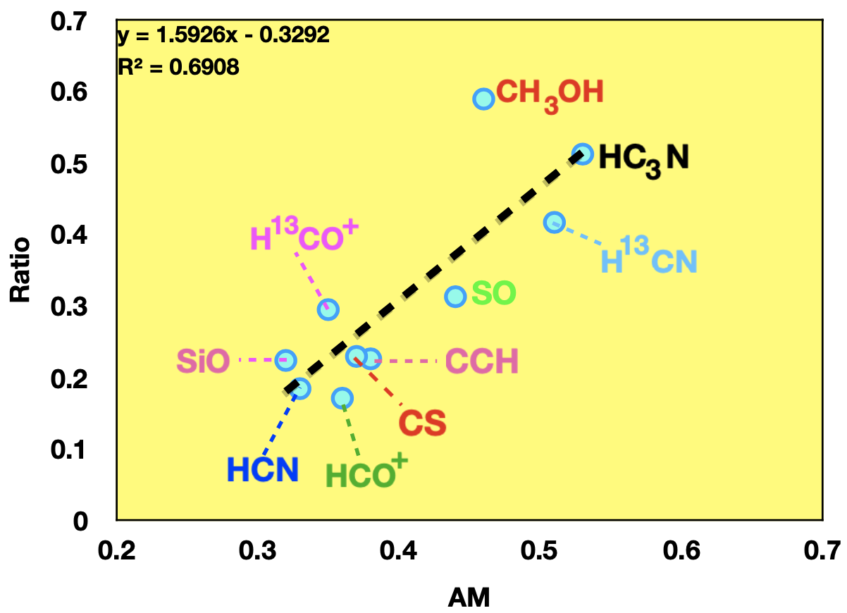
In Table 7, we compare the total integrated intensities of various molecular lines obtained from ACA measurements with that obtained from 12-m array measurements. The integrated intensities are derived in the velocity interval of 1.5 to 6.5 km s-1. The deconvolved FWHM angular sizes, peak integrated intensities and total integrated intensities () of various molecular lines in ACA data are derived from a 2D gaussian fitting, and are listed in columns 2-4 in Table 7. The total integrated intensities (S) of molecular lines in 12-m array data are measured within the massive filament region that is bounded by the 1% of peak flux density contour ( level) of the 3 mm continuum emission. We did not perform 2D Gaussian fitting on 12-m array data because the massive filament is far from a 2D Gaussian shape. We also did not measure integrated intensities of molecular lines in the Hii region “B" because there is no molecular line emission associated with it. The 1% of peak flux density contour of the 3 mm continuum emission defines well the boundary of the massive filament (see Figure 5). The ratios of to listed in the last column in Table 7 can be used to evaluate how much emission is from the densest filament region. Figure 19 shows the ratios against the values that are derived from HOGs analysis. There is a clear trend between the ratios and the values. Molecules with higher values show higher similarity with the 3 mm continuum emission. Molecules (CH3OH, HC3N and H13CN) that have high values also show high ratios of to (), further suggesting that these molecular lines are good tracers of the dense filament. In contrast, only less than 25% of the fluxes of CCH, HCN, CS and HCO+ are from the dense filament region. These molecules also show largest differences (small AM values) with the spatial distribution of the 3 mm continuum emission.
G9.62+0.19 is a gravitationally bound massive clump (Liu et al. 2017; Liu et al. 2018c). Molecular lines HCN J=1-0, CS J=2-1 and HCO+ J=1-0 are commonly used in dense gas star formation law studies (Gao & Solomon 2004; Wu et al. 2005; Wu et al. 2010). Our studies indicate that even in such a gravitationally bound clump, these commonly used lines are poor tracers of the dense structures, e.g., filament or dense cores. This is consistent with observations in nearby GMCs, where these lines do not well trace the column density structures (cores and filaments) revealed in Herschel images (Pety et al. 2017; Shimajiri et al. 2017). Our studies of G9.62+0.19 indicate that the gas lies within the dense filament as defined by the continuum emission only contributes to less than 25% flux of these lines. These main lines of dense gas tracers are poor tracers of dense structures because they tend to be optically thick in dense parts of molecular clouds (Sanhueza et al. 2012; Hoq et al. 2013; Shimajiri et al. 2017; Liu et al. 2020, e.g.,). The large optical depths of main lines, such as HCN and HCO+, indicate that the density or mass estimates from their line intensity could be misleading. In contrast to the main lines, emission from the isotopologues are optically thinner because of their much lower abundances and hence higher effective excitation densities (Shirley 2015). Therefore, they are potentially better tracers of the column densities and dense structures in molecular clouds. The optical depth issues in dense gas star formation law studies with main lines will be discussed in a companion paper by Liu et al. 2020.
In dense gas star formation law studies (Wu et al. 2010, e.g.,), the line luminosity (L) is assumed as a tracer for dense gas mass (Mdense). Wu et al. 2010 found that the median conversion factors from line luminosity to dense gas masses (L-to-Mdense) are about 20, 39, 16 and 19 M☉ (K km-1 pc2)-1 for CS J=2-1, CS J=7-6, HCN J=1-0 and HCN J=3-2 lines, respectively. In the ATOMS survey, we are more interested in how the total line luminosity of clumps correlates to the total masses (Mcores) of dense cores, i.e., the smallest star formation units. In G9.62+0.19, the total line flux densities of H13CN, H13CO+, HCN and HCO+ that are integrated over all velocity channels in ACA observations are 87, 45, 258 and 176 K km-1, respectively. We can convert the total flux densities of these lines into their line luminosity following Solomon et al. 1997. The line luminosity of the J=1-0 transitions of H13CN, H13CO+, HCN and HCO+ of the G9.62+0.19 clump are 10, 5, 29 and 19 K km-1 pc2, respectively. Liu et al. 2017 identified 12 dense cores in G9.62+0.19. The total mass of these dense cores is 400 M☉ assuming an average dust temperature of 35 K (Liu et al. 2017). Therefore, the conversion factors L-to-Mcores in G9.62+0.19 are about 40, 80, 14, and 21 M☉ (K km-1 pc2)-1 for the J=1-0 transitions of H13CN, H13CO+, HCN and HCO+, respectively. In future, we will statistically investigate the conversion factors of line luminosity to dense core masses with the full ATOMS sample, which is very helpful to investigate how star formation efficiency varies across Galactic clumps. The knowledge of these studies can also be applied to star formation in external galaxies.
4 Discussion
4.1 Stellar feedback and sequential high-mass star formation
The ATOMS aims to investigate how stellar feedback from formed OB (proto-)stars in proto-clusters affect their natal clumps and regulate new star formation. Below we discuss the stellar feedback effect in G9.62+0.19.
As discussed in section 3.2.8 and in Liu et al. 2017, sequential high-mass star formation is taking place inside the G9.62+0.19 clump, which has a size of 1 pc. The oldest Hii regions in this area seem to have great influence on their natal clump, creating a cavity in molecular line emission. From moment 1 maps (see middle panels of Figure 22 and 23) of several molecular lines (e.g., CCH, H13CO+, SO and HC3N), one can see clearly a velocity gradient across the clump. Such large-scale velocity gradient and widespread low-velocity SiO shocks surrounding the Hii regions are more likely caused by the expansion of the Hii region "B". It indicates that stellar feedback from formed OB proto-stars can greatly reshape their natal clumps and change the spatial distribution of gas.
We also noticed that the evolved OB proto-stars in G9.62+0.19 are not located near the center of the clump but are clearly close to the clump edges. Along the massive filament, most evolved sources are located at the ends and the youngest sources are located in the filament center. This phenomenon is similar to the "edge-collapse" process proposed for filaments (Pon et al. 2011; Pon et al. 2012; Clarke & Whitworth 2015). For long filaments with aspect ratios larger than 2, the global collapse of the filaments is likely end-dominated (Clarke & Whitworth 2015). The ends experience the highest acceleration, and this leads to the formation of end-clumps which then converge on the centre. In addition, recent ALMA high-resolution observations of massive infrared dark clouds (IRDCs) indicate that there is no significant evidence of primordial mass segregation (Contreras et al. 2018; Sanhueza et al. 2019). More massive cores are distributed in the same way as other low-mass cores (Contreras et al. 2018; Sanhueza et al. 2019). The observations of those IRDCs are consistent with what we have found here in the G9.62+0.19 clump. It seems that high-mass stars are not necessarily formed at the clump center as expected by the "competitive accretion" model (Bonnell et al. 2002; Bonnell & Bate 2006; Bonnel 2008). Recently, Padoan et al. 2019 proposed a new scenario of massive-star formation, the "Inertial-Inflow Model", in which massive stars are assembled by large-scale, converging, inertial flows that naturally occur in supersonic turbulence.

Based on our knowledge of the G9.62+0.19 clump and recent studies of IRDCs, we propose the following scenario to explain the sequential high-mass star formation in pc-size clumps. The sketch of the scenario is shown in Figure 20. The three stages involved in proto-cluster formation of this scenario are:
(a) The initial fragmentation of a massive clump does not show significant evidence of primordial mass segregation (Sanhueza et al. 2019). The clumps are accreting gas from large-scale converging flows (Padoan et al. 2019). These flows generate low-velocity shocks that excite widespread narrow SiO emission.
(b) As proposed in the "edge-collapse" scenario (Pon et al. 2011; Pon et al. 2012; Clarke & Whitworth 2015), dense cores that are near the clump edges or at the ends of dense filaments inside clumps have higher accretion rates and are more gravitationally unstable. They will be the first to collapse to form proto-stars. Dense cores and formed proto-stars keep accreting gas from clump gas. High-mass proto-stars could form away from clump center as seen in the G9.62+0.19 complex.
(c) Stellar feedback from formed OB stars reshapes their natal clumps and changes the spatial distribution of gas and dense cores. The expansion of Hii regions can also generate low-velocity shocks that excite widespread narrow SiO emission in their surroundings. Some low-mass dense cores could be destroyed as Hii regions expand into the clump. Some dense cores in front of Hii regions may collide and merge into massive cores or massive filament due to the enhanced density by the Hii region shocks. This can explain the lack of widespread low-mass cores in the G9.62+0.19 complex (Liu et al. 2017). New generation of high-mass proto-stars could form in these new massive cores.
Statistical studies of a large number of proto-clusters in the ATOMS survey will help test this scenario.
4.2 Links to other surveys
There are several on-going or completed survey programs aiming at studying dense gas in either Galactic Giant molecular clouds or external galaxies. In this section, we will introduce several of these surveys and discuss how they will connect to the ATOMS survey.
The "Millimetre Astronomy Legacy Team 90 GHz (MALT90)" survey (PI: J. M. Jackson) has used the Mopra 22-m single-dish telescope to obtain maps in various gas tracers towards 2000 dense molecular clumps that are at different evolutionary stages (Jackson et al. 2013; Sanhueza et al. 2012; Stephens et al. 2016). The "MALT90" project aims to characterize the physical and chemical evolution of high-mass star-forming clumps. The "ATOMS" survey observed similar gas tracers as in the "MALT90" project, e.g., HCN, HCO+, and their isotopologue lines, CCH, SiO, and HC3N. The "ATOMS" survey data will be used to study the star formation scaling relations (Liu et al. 2020), and compared with those derived using "MALT90" data (Stephens et al. 2016). The "ATOMS" survey has a much higher angular resolution (2 vs. 38) than the "MALT90" project. The "ATOMS" survey will reveal the internal structures and detailed spatial gas distributions within the Galactic clumps that cannot be resolved in the "MALT90" project.
The "Orion B: The Anatomy of a Giant Molecular Cloud" (PI: J. Pety) is a multi-line imaging survey at the IRAM 30-m telescope toward the Orion B molecular cloud (Pety et al. 2017). It covers approximately thirty 3 mm lines with a typical resolution of 26 (or 0.05 pc at Orion distance). The "Orion B" project aims to obtain an accurate 3D description of the molecular structure in a GMC and to reveal the detailed anatomy of a molecular emission that is usually hidden behind these galaxy-averaged spectra in nearby galaxy studies. The ATOMS survey has comparable or better spatial resolution (0.05 pc) than the "Orion B" project for the 98 targeted Galactic clumps within 5 kpc. The ATOMS survey aims to reveal the detailed spatial distributions of molecular line emission inside a large sample of Galactic clumps and shares similar science goals as the "Orion B" project. The comparative studies with the "Orion B" data and the "ATOMS" data will shed light on the spatial distributions of molecular emission across a widely different environment from a nearby GMC to distant massive star forming regions.
The "EMIR Multiline Probe of the ISM Regulating Galaxy Evolution" (EMPIRE; PI: Frank Bigiel) survey is a multi-line mapping survey at the IRAM 30-m telescope that is targeting high critical density molecular lines (=1-0 of HCN, HCO+ and HNC) and CO isotopologues across the disks of 9 nearby, star-forming, disk galaxies (Jiménez-Donaire et al. 2019). With an angular resolution of 30 at 90 GHz (or 1-2kpc), The EMPIRE survey aims to constrain dense gas fraction and star formation efficiency across galaxy disks and explore how they depend on local conditions (molecular fraction, hydrostatic pressure, radiation field, stellar potential, etc.). The ATOMS survey also aims to investigate the star formation scaling relations with the same high critical density gas tracers, e.g., =1-0 of HCN, HCO+ and their isotopologue lines, and also to study how star formation efficiency changes across the inner Galaxy. The joint analysis of the ATOMS data and "EMPIRE" data will link "dense gas" from the Milky Way to external galaxies.
The "ALMA_IMF: ALMA transforms our view of the origin of stellar masses" (PI: Frédérique Motte) observed 15 most massive clouds within 6 kpc at 3 mm and 1.3 mm at the 2000 AU spatial resolution. The "ALMA_IMF" project aims to constrain the protocluster core mass function (CMF) in the range 0.5-200 M☉ and to investigate which variables (such as inflows, outflows, or forming filaments) might be correlated with CMF evolution in proto-clusters. In contrast, the desired 3 mm continuum rms level in the ATOMS survey is of 65 Jy, corresponding to a mass sensitivity 2 M☉ at a distance of 1 kpc and 50 M☉ at a distance of 5 kpc (Kauffmann et al. 2008). The mass sensitivity is derived with a median dust temperature of 30 K and a dust opacity per unit gas mass of 0.00189 cm2 g-1 at 3 mm that is extrapolated from the dust opacity of 0.01 cm2 g-1 at 230 GHz assuming a dust opacity index () of 2 (Ossenkopf& Henning 1994). Therefore, the ATOMS project will help constrain the high-mass end of the CMFs in protoclusters with a much larger sample but a shallower mass sensitivity than the "ALMA_IMF" project.
Another ALMA survey project, "ALMAGAL: ALMA Evolutionary study of High Mass Protocluster Formation in the Galaxy" (PI: Sergio Molinari), will observe more than 1000 dense clumps with M500 M☉ and d7.5 kpc with similar linear resolution ( AU) and a mass sensitivity of 0.3 M☉ at 1.3 mm. The "ALMAGAL" project will systematically investigate what the physical characteristics of core fragments in dense clumps are as a function of evolution and to what extent fragmentation is driven by dynamics in clumps or mass transport in filaments. The angular resolution and mass sensitivity of the "ALMAGAL" project are much better than the ATOMS project. However, the ATOMS survey benefits from the (3 times) larger FOV at 3 mm than that of the "ALMAGAL" project at 1.3 mm, indicating that the ATOMS survey are more suitable to study the overall structures and kinematics in proto-clusters. The comparative studies with the "ALMAGAL" data and the "ATOMS" data will help deepen the understandings of hierarchical fragmentation and differential star formation in high-mass proto-clusters.
5 Conclusions
We introduce in this paper the observations, data reduction and example science case, G9.62+0.19 (I18032-2032), of the ALMA survey program ATOMS. The ATOMS project, standing for ALMA Three-millimeter Observations of Massive Star-forming regions, has observed 146 active star forming regions at Band 3 in both continuum emission and molecule lines. More than 90% of the "ATOMS" targeted sources are promising high-mass star forming regions. The ATOMS survey aims to systematically investigate the spatial distribution of various dense gas tracers, the roles of stellar feedback and filaments in star formation.
(1) The 3 mm continuum data of the ATOMS survey will be used to detect massive filaments and dense cores. In G9.62+0.19, the 3 mm continuum emission reveals an expanding Hii region "B" to the west and a massive fragmented filament to the east. The 3 mm continuum emission of the expanding Hii region "B", compact Hii region "MM1/C" and the UC Hii region "M11/D" seem to be dominated by free-free emission.
(2) The "ATOMS" survey covers dozens of molecular line transitions, including shocked gas tracers (SiO, SO), a PDR tracer (CCH), hot core tracers (e.g., HC3N and CH3OH) and some lines commonly assumed to trace dense gas (e.g., HCN, HCO+ and CS). It also includes a tracer of ionized gas (H40α recombination line). We will investigate the spatial distributions of various gas tracers within a large sample of massive clumps. In G9.62+0.19, the similarities and differences in images of 10 molecular lines in Table 2 are investigated with the principal component analysis and the histogram of oriented gradients analysis. We found that the 10 lines can be classified into three groups. The first group includes CS, HCO+, HCN, CCH and H13CO+, which mainly trace extended gas emission. SiO in the second group stands out from other molecules because it mainly traces shocked gas. The third group including SO, CH3OH, H13CN and HC3N traces well dense gas in the massive filaments. Molecules in the same group show strongest correlations in their spatial distribution. SO, CH3OH, H13CN and HC3N show morphology similar to that of the 3 mm continuum emission. The other molecular lines including the commonly used dense gas tracers, e.g., CS J=2-1, J=1-0 of HCO+ and HCN, can not reveal well dense structures (dense cores and filament) in G9.62+0.19 on the scale of 0.1 pc.
(3) In the ATOMS survey, we will for the first time investigate statistically the origin of various velocity shocks using shock tracers like SiO. In G9.62+0.19, SiO shows widespread narrow emission, which is likely caused by slow shocks generated by large-scale colliding flows and Hii regions.
(4) In the ATOMS survey, we will identify outflows driven by proto-stars. For G9.62+0.19, SiO, SO, CS, HCO+ and HCN trace well high-velocity outflow gas emission. The outflows, as traced by these molecular lines, show very similar morphology.
(5) The ATOMS survey covers a wide frequency range that includes dozens of molecular transitions that can be used to study chemical differentiation among dense cores. In G9.62+0.19, three dense cores (MM4/E, MM7/G and MM8/F) show hot core chemistry.
(6) The ATOMS survey aims to statistically evaluate what fraction of gas in gravitationally bound clumps is actually participating in star formation or is concentrated in the smallest star formation units, i.e., dense cores. In G9.62+0.19, only less than 25% of the "dense gas" revealed by HCN, CS and HCO+ is concentrated in the massive filament.
(7) The ATOMS survey aims to investigate how stellar feedback from formed OB (proto-)stars in proto-clusters affect their natal clumps and star formation efficiency. Stellar feedback from formed OB stars (Hii region "B") in G9.62+0.19 has reshaped their natal clump and changed the spatial distribution of gas and dense cores. Stellar feedback may be also the cause of the sequential high-mass star formation that is taking place in G9.62+0.19 complex.
(8) Joint analysis with the ATOMS survey data and other survey data, such as "MALT90", "Orion B", "EMPIRE", "ALMA_IMF", and "ALMAGAL", will help deepen our understandings of "dense gas" star formation scaling relations and massive proto-cluster formation.
Acknowledgements
Tie Liu is supported by the initial funding of scientific research for high-level talents at Shanghai Astronomical Observatory. This work was carried out in part at the Jet Propulsion Laboratory, which is operated for NASA by the California Institute of Technology. LB acknowledges support from CONICYT project Basal AFB-170002. Di Li is supported by CAS International Partnership Program No.114A11KYSB20160008. This paper makes use of the following ALMA data: ADS/JAO.ALMA#2019.1.00685.S. ALMA is a partnership of ESO (representing its member states), NSF (USA) and NINS (Japan), together with NRC (Canada), MOST and ASIAA (Taiwan), and KASI (Republic of Korea), in cooperation with the Republic of Chile. The Joint ALMA Observatory is operated by ESO, AUI/NRAO and NAOJ.
References
- Aladro et al. (2015) Aladro, R., Martín, S., Riquelme, D., et al. 2015, A&A, 579, A101
- Allen et al. (2017) Allen, V., van der Tak, F. F. S., Sánchez-Monge, Á., et al., 2017, A&A, 603A, 133A
- André et al. (2010) André, P., Men’shchikov, A., Bontemps, S., et al., 2010,A&A, 518L, 102A
- André et al. (2014) André, P.; Di Francesco, J.; Ward-Thompson, D., et al.,2014, Protostars and Planets VI, 914 pp., p.27-51
- André et al. (2019) André, P., Arzoumanian, D., Könyves, V., et al.,2019, A&A, 629, L4
- Arzoumanian et al. (2011) Arzoumanian, D., André, Ph., Didelon, P., et al., 2011, A&A, 529L, 6A
- Arzoumanian et al. (2019) Arzoumanian, D., André, P., Könyves, V., et al. 2019, A&A, 621A, 42A
- Berry et al. (2015) Berry, D. S. 2015, A&C, 10, 22
- Berry et al. (2007) Berry, D. S., Reinhold, K., Jenness, T., & Economou, F. 2007, in ASP Conf. Ser. 376, Astronomical Data Analysis Software and Systems XVI, ed. R. A. Shaw, F. Hill, & D. J. Bell (San Francisco, CA: ASP), 425
- Barnes et al. (2016) Barnes, P. J., Hernandez, A. K., O’Dougherty, S. N., 2016, ApJ, 831, 67
- Beuther et al. (2008) Beuther, H., Semenov, D., Henning, T., & Linz, H. 2008, ApJ, 675, L33
- Bigiel et al. (2008) Bigiel, F., Leroy, A., Walter, F., et al. 2008, AJ, 136, 2846
- Bonnell et al. (2002) Bonnell, I. A., Bate, M. R., Clarke, C. J., Pringle, J. E., 2002, MNRAS, 323, 785
- Bonnell & Bate (2006) Bonnell, I. A. & Bate, M. R., 2006, MNRAS, 370, 488
- Bonnel (2008) Bonnell, I. A., 2008, ASPC, 390, 26
- Bressert et al. (2012) Bressert, E., Ginsburg, A., Bally, J., et al. 2012, ApJ, 758, L28
- Bronfman et al. (1996) Bronfman, L., Nyman, L. -A., May, J., 1996, A&AS, 115, 81
- Clarke & Whitworth (2015) Clarke, S. D. & Whitworth, A. P. 2015, MNRAS, 449, 1819
- Chen et al. (2015) Chen, H., Gao, Y., Braine, J., et al., 2015, ApJ, 810, 140
- Chen et al. (2019) Chen, H., Zhang, Q., Wright, M. C. H., et al., 2019, ApJ, 875, 24
- Chen et al. (2008) Chen, X., Bourke, T. L., Launhardt, R., et al. 2008, ApJ, 686L, 107
- Condon & Ransom (2016) Condon, J. J., & Ransom, S. M. 2016, Essential Radio Astronomy (Princeton, NJ: Princeton Univ. Press)
- Contreras et al. (2018) Contreras, Y., Sanhueza, P., Jackson, J. M., et al., 2018, ApJ, 861, 14
- Cosentino et al. (2018) Cosentino, G., Jiménez-Serra, I., Henshaw, J. D., et al., 2018, MNRAS, 474, 3760
- Cosentino et al. (2019) Cosentino, G., Jiménez-Serra, I., Caselli, P., et al., 2019, ApJ, 881L, 42C
- Cuadrado et al. (2015) Cuadrado, S., Goicoechea, J. R., Pilleri, P., et al. 2015, A&A, 575, A82
- Dall’Olio et al. (2019) Dall’Olio, D., Vlemmings, W. H. T., Persson, M. V., et al., 2019, A&A, 626A, 36D
- Dobbs et al. (2011) Dobbs, C. L., Burkert, A., Pringle, J. E., 2011, MNRAS, 413, 2935
- Eden et al. (2017) Eden, D. J., Moore, T. J. T., Plume, R., et al. 2017, MNRAS, 469, 2163
- Eden et al. (2019) Eden, D. J., Liu, T., Kim, K.-T., et al., 2019, MNRAS, 485, 2895
- Elmegreen & Lada (1977) Elmegreen, B. G., & Lada, C. J. 1977, ApJ, 214, 725
- Enoch et al. (2007) Enoch, M. L., Glenn, J., Evans, N. J., II, et al., 2007, ApJ, 666, 982
- Esplugues et al. (2013) Esplugues, G. B., Tercero, B., Cernicharo, J., 2013, A&A, 556A, 143E
- Evans (1999) Evans, N. J., II 1999, ARA&A, 37, 311
- Evans et al. (2014) Evans, Neal J., II, Heiderman, A., Vutisalchavakul, N., 2014, ApJ, 782, 114
- Evans et al. (2020) Evans, Neal J., II, Kim, K.-T., Wu, J.-W., 2020, ApJ, 894, 103
- Faúndez et al. (2004) Faúndez, S., Bronfman, L., Garay, G., et al. 2004, A&A, 426, 97
- Gao & Solomon (2004) Gao, Y., & Solomon, P. M. 2004, ApJ, 606, 271
- Garay et al. (1993) Garay, G., Rodriguez, L. F., Moran, J. M., & Churchwell, E., 1993, ApJ, 418, 368
- Ginsburg et al. (2013) Ginsburg, A., Glenn, J., Rosolowsky, E., et al., 2013, ApJS, 208, 14
- Goicoechea et al. (2016) Goicoechea, J. R., Pety, J., Cuadrado, S., 2016, Nature, 537, 207
- González Lobos & Stutz (2019) González Lobos, V., & Stutz, A. M. 2019, MNRAS, 489, 4771
- Greve (2014) Greve, T. R., Leonidaki, I., Xilouris, E. M., et al. 2014, ApJ, 794, 142
- Heiderman et al. (2010) Heiderman, A., Evans, N. J. II, Allen, L. E., et al., 2010, ApJ, 723, 1019
- Hacar et al. (2013) Hacar, A., Tafalla, M., Kauffmann, J., et al., 2013, A&A, 554A, 55H
- Hacar et al. (2016) Hacar, A., Kainulainen, J.; Tafalla, M., et al., 2016, A&A, 587A, 97H
- Hacar et al. (2018) Hacar, A., Tafalla, M., Forbrich, J., et al., 2018, A&A, 610A, 77H
- Hofner et al. (1994) Hofner, P., Kurtz, S., Churchwell, E., Walmsley, C. M., & Cesaroni, R., 1994, ApJ, 429, L85
- Hofner et al. (1996) Hofner, P., Kurtz, S., Churchwell, E., Walmsley, C. M., & Cesaroni, R., 1996, ApJ, 460, 359
- Hofner, Wiesemeyer, & Henning (2001) Hofner, P., Wiesemeyer, H., & Henning, T., 2001, ApJ, 549, 425
- Jackson et al. (2013) Jackson, J. M., Rathborne, J. M., Foster, J. B., 2013, Publ. Astron. Soc. Australia, 30, 57
- Jiménez-Serra et al. (2010) Jiménez-Serra, I., Caselli, P., Tan, J. C., et al., 2010, MNRAS, 406, 187
- Jiménez-Donaire et al. (2019) Jiménez-Donaire, María J., Bigiel, F., Leroy, A. K., 2019, ApJ, 880, 127
- Jones et al. (2012) Jones, P. A., Burton, M. G., Cunningham, M. R., et al., 2012, MNRAS, 419, 2961
- Jones et al. (2013) Jones, P. A., Burton, M. G., Cunningham, M. R., et al., 2013, MNRAS, 433, 221
- Juvela et al. (2012) Juvela, M., Ristorcelli, I., Pagani, L., et al., 2012, 541A, 12J
- Kainulainen et al. (2017) Kainulainen, J., Stutz, A. M., Stanke, T., et al. 2017, A&A, 600, A141
- Kauffmann et al. (2008) Kauffmann, J., Bertoldi, F., Bourke, T. L., 2008, A&A, 487, 993
- Kauffmann & Pillai (2010) Kauffmann, J., & Pillai, T. 2010, ApJ, 723, L7
- Kauffmann et al. (2017) Kauffmann, J., Goldsmith, P. F., Melnick, G., et al., 2017, A&A, 605, L5
- Kennicutt (1998a) Kennicutt, R. C., Jr. 1998a, ApJ, 498, 541
- Kennicutt (1998b) Kennicutt, R. C., Jr. 1998b, ARA&A, 36, 189
- Kennicutt & Evans (2012) Kennicutt, R. C., & Evans, N. J. 2012, ARA&A, 50, 531
- Kirk et al. (2013) Kirk, H., Myers, P. C., Bourke, T. L., et al. 2013, ApJ, 766, 115
- Krumholz & McKee (2008) Krumholz, M. R., & McKee, C. F. 2008, Nature, 451, 1082
- Krumholz et al. (2011) Krumholz, M. R., Klein, R. I., McKee, C. F., 2011, ApJ, 740, 74
- Krumholz et al. (2014) Krumholz, M. R., Bate, M. R., Arce, H. G., et al., 2014, Protostars and Planets VI, Henrik Beuther, Ralf S. Klessen, Cornelis P. Dullemond, and Thomas Henning (eds.), University of Arizona Press, Tucson, 914 pp., p.243-266
- Hoq et al. (2013) Hoq, S., Jackson, J. M., Foster, J. B., et al., 2013, ApJ, 777, 157
- Könyves et al. (2015) Könyves, V., André, Ph., Men’shchikov, A., et al., 2015, A&A, 584A, 91K
- Lada et al. (2012) Lada, C. J., Forbrich, J., Lombardi, M., et al. 2012, ApJ, 745, 190
- Lada et al. (2010) Lada, C. J., Lombardi, M., & Alves, J. F. 2010, ApJ, 724, 687
- Lazarian & Hoang (2007) Lazarian, A., & Hoang, T. 2007, MNRAS, 378, 910
- Le Page et al. (2003) Le Page, V., Snow, T. P., & Bierbaum, V. M. 2003, ApJ, 584, 316
- Liu et al. (2015) Liu, D., Gao, Y., Isaak, K., et al. 2015, ApJ, 810L, 14L
- Liu et al. (2012) Liu, H. B., Jiménez-Serra, I., Ho, P. T. P., et al. 2012, ApJ, 756, 10
- Liu et al. (2015b) Liu, H. B., Galván-Madrid, R., Jiménez-Serra, I., et al. 2015b, ApJ, 804, 37
- Liu et al. (2019) Liu, H. B., Chen, H.-R. V., Román-Zúñiga, C. G., 2019, ApJ, 871, 185
- Liu et al. (2011) Liu, T., Wu, Y., Liu, S.-Y., et al. 2011, ApJ, 730, 102
- Liu et al. (2016) Liu, T., Kim, K.-T., Yoo, H., et al., 2016, ApJ, 829, 59
- Liu et al. (2017) Liu, T., Lacy, J., Li, P. S., et al., 2017, ApJ, 849, 25
- Liu et al. (2018a) Liu, T., Kim, K.-T., Juvela, M., et al., 2018a, ApJS, 234, 28L
- Liu et al. (2018b) Liu, T., Li, P. S., Juvela, M., et al., 2018b, ApJ, 859, 151L
- Liu et al. (2018c) Liu T., et al., 2018, ApJ, 869, L5
- Liu et al. (2020) Liu, T., Evans, N., Kim, K.-T., et al., 2020, accepted to MNRAS, 496, 2790
- Lo et al. (2009) Lo, N., Cunningham, M. R., Jones, P. A., et al., 2009, 395, 1021
- Louvet et al. (2016) Louvet, F., Motte, F., Gusdorf, A., et al., 2016, A&A, 595A, 122L
- Lu et al. (2018) Lu, X., Zhang, Q., Liu, H. B., et al. 2018, ApJ, 855, 9
- Moscadelli et al. (2018) Moscadelli, L., Rivilla, V. M., Cesaroni, R., et al., 2018, A&A, 616A, 66M
- Molinari et al. (2008) Molinari, S., Pezzuto, S., Cesaroni, R., et al. 2008, A&A, 481, 345
- Molinari et al. (2010) Molinari, S., Swinyard, B., Bally, J., et al., 2010, A&A, 518L, 100M
- McMullin et al. (2007) McMullin, J. P., Waters, B., Schiebel, D., et al. 2007, adass XVI, 127
- Möller et al. (2017) Möller, T., Endres, C., Schilke, P., 2017, A&A, 598, A7
- Montillaud et al. (2013) Montillaud, J., Joblin, C., & Toublanc, D. 2013, A&A, 552, A15
- Myers et al. (2013) Myers, A. T., McKee, C. F., Cunningham, A. J., et al., 2013, ApJ, 766, 97
- Nagy et al. (2019) Nagy, Z., Spezzano, S., Caselli, P., et al., 2019, A&A, 630A, 136N
- Nguyen-Lu’o’ng et al. (2013) Nguyen-Lu’o’ng, Q., Motte, F., Carlhoff, P., et al., 2013, ApJ, 775, 88
- Nguyen-Luong et al. (2020) Nguyen-Luong, Q., Nakamura, F., Sugitani, K., et al., 2020, ApJ, 891, 66
- Offner et al. (2009) Offner, S. S. R., Klein, R. I., McKee, C. F., 2009, ApJ, 703, 131
- Ossenkopf& Henning (1994) Ossenkopf, V., & Henning, T. 1994, A&A, 291, 943
- Padoan et al. (2019) Padoan, P., Pan, L., Juvela, M., et al., 2019, ApJ, in press, arXiv:1911.04465
- Papadopoulos (2007) Papadopoulos, Padeli P. 2007, ApJ, 656, 792
- Peng et al. (2019) Peng, Y., Rivilla, V. M., Zhang, L., et al., 2019, ApJ, 871, 251
- Peng et al. (2017) Peng, Y., Qin, S.-L., Schilke, P., et al., 2017, ApJ, 837, 49
- Peretto et al. (2013) Peretto, N., Fuller, G. A., Duarte-Cabral, A., et al. 2013, A&A, 555, 112
- Pety et al. (2005) Pety, J., Teyssier, D., Fossé, D., et al. 2005, A&A, 435, 885
- Pety et al. (2017) Pety, J., Guzmán, V. V., Orkisz, J. H., et al., 2017, A&A, 599, A98
- Pols et al. (2018) Pols, S., Schwörer, A., Schilke, P., et al., 2018, A&A, 614A, 123P
- Pon et al. (2011) Pon, A., Johnstone, D., & Heitsch, F. 2011, ApJ, 740, 88
- Pon et al. (2012) Pon, A., Toalá, J. A., Johnstone, D., et al. 2012, ApJ, 756, 145
- Pratap et al. (1997) Pratap, P., Dickens, J. E., Snell, R. L., et al. 1997, ApJ, 486, 862
- Qin et al. (2015) Qin, S.-L., Schilke, P., Wu, J., et al., 2015, ApJ, 803, 39
- Quireza et al. (2006) Quireza, C., Rood, R. T.; Bania, T. M., et al., 2006, ApJ, 653, 1226
- Sanna et al. (2009) Sanna, A., Reid, M. J., Moscadelli, L., Dame, T. M., Menten, K. M., Brunthaler, A., Zheng, X. W., Xu, Y., 2009, ApJ, 706, 464
- Sanhueza et al. (2012) Sanhueza, P., Jackson, J. M., Foster, J. B., et al., 2012, ApJ, 756, 60
- Sanhueza et al. (2019) Sanhueza, P., Contreras, Y., Wu, B., et al., 2019, ApJ, 886, 102
- Saraceno et al. (1996) Saraceno, P., Andre, P., Ceccarelli, C., Griffin, M., & Molinari, S. 1996, A&A, 309, 827
- Schisano (2020) Schisano, E., Molinari, S., Elia, D., et al., 2020, MNRAS, 492, 5420
- Schmidt (1959) Schmidt, M. 1959, ApJ, 129, 243
- Silk (1997) Silk, J. 1997, ApJ, 481, 703
- Shimajiri et al. (2017) Shimajiri, Y., André, P., Braine, J., et al., 2017, A&A, 604, A74
- Shirley (2015) Shirley, Yancy L., 2015, PASP, 127, 299
- Soler et al. (2019) Soler, J. D., Beuther, H., Rugel, M.,et al., 2019, A&A, 622A, 166S
- Solomon et al. (1997) Solomon, P. M., Downes, D., Radford, S. J. E., & Barrett, J. W. 1997, ApJ, 478, 144
- Spezzano et al. (2017) Spezzano, S., Caselli, P., Bizzocchi, L., 2017, A&A, 606A, 82S
- Stephens et al. (2016) Stephens, I. W., Jackson, J. M., & Whitaker, J. S. 2016, ApJ, 824, 29
- Stutz & Gould (2016) Stutz, A. M., & Gould, A. 2016, A&A, 590, A2
- Stutz (2018) Stutz, A. M. 2018, MNRAS, 473, 4890
- Tacconi et al. (2020) Tacconi, L. J., Genzel, R., & Sternberg, A., 2020, ARA&A, in press, eprint arXiv:2003.06245
- Testi et al. (2000) Testi, L., Hofner, P., Kurtz, S., & Rupen, M., 2000, A&A, 359, L5
- Tiwari et al. (2019) Tiwari, M., Menten, K. M., Wyrowski, F., et al., 2019, A&A, 626A, 28T
- Thompson et al. (2012) Thompson, M. A., Urquhart, J. S., Moore, T. J. T., et al., 2012, MNRAS, 421, 408
- Tan et al. (2018) Tan, Q., Gao, Y., Zhang, Z.-Y. et al., 2018, ApJ, 860, 165
- Tobin et al. (2019) Tobin, J. J., Bourke, T. L., Mader, S., 2019, ApJ, 870, 81
- Urquhart et al. (2014) Urquhart, J. S., Moore, T. J. T., Csengeri, T., et al. 2014, MNRAS, 443, 1555
- Urquhart et al. (2018) Urquhart, J. S., König, C., Giannetti, A., 2018, MNRAS, 473, 1059
- Vutisalchavakul et al. (2016) Vutisalchavakul, N., Evans, N. J., II, Heyer, M., 2016, ApJ, 831, 73
- Wang et al. (2011) Wang, K., Zhang, Q., Wu, Y., 2011, ApJ, 735, 64W
- Wang et al. (2014) Wang, K., Zhang, Q., Testi, L., et al., 2014, MNRAS, 439, 3275
- Wang et al. (2012) Wang, K., Zhang, Q., Wu, Y., 2012, ApJ, 745L, 30
- Wang et al. (2016) Wang, K., Testi, L., Burkert, A., et al. 2016, ApJS, 226, 9
- Wall et al. (2020) Wall, J. E., Mac Low, M., McMillan, S. L. W., et al., 2020, submitted, arXiv:2003.09011
- Whitworth et al. (1994a) Whitworth, A. P., Bhattal, A. S., Chapman, S. J., et al., 1994a, A&A, 290, 421
- Whitworth et al. (1994b) Whitworth, A. P., Bhattal, A. S., Chapman, S. J., et al., 1994b, MNRAS, 268, 291
- Wu et al. (2005) Wu, J., Evans, N. J., II, Gao, Y., et al. 2005, ApJ, 635, L173
- Wu et al. (2010) Wu, J., Evans, N. J., II, Shirley, Y. L., et al. 2010, ApJS, 188, 313
- Yuan et al. (2017) Yuan, J., Wu, Y., Ellingsen, S. P., et al., 2017, ApJS, 231, 11
- Zhang & Wang (2011) Zhang, Q., & Wang, K. 2011, ApJ, 733, 26
- Zhang et al. (2015) Zhang, Q., Wang, K., Lu, X., 2015, ApJ, 804, 141
- Zhang et al. (2014) Zhang, Z.-Y., Gao, Y., Henkel, C., et al. 2014, ApJL, 784, L31
- Zhu et al. (2019) Zhu, F.-Y., Zhu, Q.-F., Wang, J.-Z., et al., 2019, ApJ, 881, 14
Appendix A
| ID | IRAS | RA | DEC | Vlsr | Distance | Radius | log() | log() | refsa | ||
| (km s-1) | (kpc) | (kpc) | (pc) | (K) | (L☉) | (M☉) | |||||
| 1 | I08076-3556 | 08:09:32.39 | -36:05:13.2 | 5.9 | 0.4 | 8.5 | 0.07 | 18.0 | 1.2 | 0.7 | 1 |
| 2 | I08303-4303 | 08:32:08.34 | -43:13:54.0 | 14.3 | 2.3 | 9.0 | 0.32 | 30.0 | 3.8 | 2.4 | 1 |
| 3 | I08448-4343 | 08:46:32.90 | -43:54:35.9 | 3.7 | 0.7 | 8.4 | 0.15 | 25.0 | 3.0 | 1.6 | 1 |
| 4 | I08470-4243 | 08:48:47.07 | -42:54:31.0 | 12 | 2.1 | 8.8 | 0.32 | 33.0 | 4.0 | 2.4 | 1 |
| 5 | I09002-4732 | 09:01:54.24 | -47:44:00.8 | 3.1 | 1.2 | 8.4 | 0.24 | 39.0 | 4.6 | 2.4 | 1 |
| 6 | I09018-4816 | 09:03:32.84 | -48:28:10.0 | 10.3 | 2.6 | 8.8 | 0.44 | 31.0 | 4.7 | 3.0 | 1 |
| 7 | I09094-4803 | 09:11:07.29 | -48:15:48.7 | 74.6 | 9.6 | 12.7 | 1.40 | 23.0 | 4.6 | 3.1 | 1 |
| 8 | I10365-5803 | 10:38:32.46 | -58:19:05.9 | -19 | 2.4 | 8.0 | 0.44 | 30.0 | 4.3 | 2.7 | 1 |
| 9 | I11298-6155 | 11:32:05.70 | -62:12:24.3 | 32.9 | 10 | 10.1 | 1.36 | 32.0 | 5.2 | 3.4 | 1 |
| 10 | I11332-6258 | 11:35:31.81 | -63:14:44.6 | -15.4 | 1.9 | 7.7 | 0.28 | 30.0 | 3.7 | 2.1 | 1 |
| 11 | I11590-6452 | 12:01:34.54 | -65:08:52.9 | -4.3 | 0.4 | 8.2 | 0.06 | 22.0 | 1.7 | 1.1 | 1 |
| 12 | I12320-6122 | 12:34:53.38 | -61:39:46.9 | -42.5 | 3.43 | 7.2 | 1.00 | 44.6 | 5.6 | 3.0 | 2 |
| 13 | I12326-6245 | 12:35:34.81 | -63:02:32.1 | -39.6 | 4.61 | 7.2 | 0.83 | 34.2 | 5.4 | 3.5 | 2 |
| 14 | I12383-6128 | 12:41:17.32 | -61:44:38.6 | -39.1 | 3.27 | 7.2 | 0.63 | 19.8 | 3.8 | 3.1 | 2 |
| 15 | I12572-6316 | 13:00:24.43 | -63:32:30.4 | 30.9 | 11.57 | 9.8 | 1.63 | 21.5 | 4.6 | 3.9 | 2 |
| 16 | I13079-6218 | 13:11:14.16 | -62:34:42.1 | -42.6 | 3.8 | 6.9 | 1.09 | 28.2 | 5.1 | 3.5 | 2 |
| 17 | I13080-6229 | 13:11:14.10 | -62:45:01.9 | -35.6 | 3.8 | 6.9 | 1.03 | 34.1 | 5.1 | 3.2 | 2 |
| 18 | I13111-6228 | 13:14:26.43 | -62:44:24.1 | -38.8 | 3.8 | 6.9 | 0.96 | 30.0 | 4.8 | 3.1 | 2 |
| 19 | I13134-6242 | 13:16:43.05 | -62:58:30.1 | -31.5 | 3.8 | 6.9 | 0.57 | 29.2 | 4.6 | 3.1 | 2 |
| 20 | I13140-6226 | 13:17:15.70 | -62:42:27.5 | -33.9 | 3.8 | 6.9 | 0.50 | 22.6 | 3.8 | 2.9 | 2 |
| 21 | I13291-6229 | 13:32:32.38 | -62:45:23.5 | -36.5 | 2.9 | 7.0 | 0.55 | 28.8 | 4.3 | 2.7 | 2 |
| 22 | I13291-6249 | 13:32:31.23 | -63:05:21.8 | -34.7 | 7.61 | 7.1 | 1.73 | 27.2 | 5.2 | 3.7 | 2 |
| 23 | I13295-6152 | 13:32:53.49 | -62:07:49.3 | -44.4 | 3.89 | 6.7 | 0.36 | 19.4 | 3.3 | 2.7 | 2 |
| 24 | I13471-6120 | 13:50:42.10 | -61:35:14.9 | -56.7 | 5.46 | 6.4 | 1.01 | 35.1 | 5.3 | 3.4 | 2 |
| 25 | I13484-6100 | 13:51:58.64 | -61:15:43.3 | -55 | 5.4 | 6.4 | 0.84 | 31.8 | 4.8 | 3.1 | 2 |
| 26 | I14013-6105 | 14:04:54.56 | -61:20:10.7 | -48.1 | 4.12 | 6.4 | 0.80 | 31.4 | 5.0 | 3.2 | 2 |
| 27 | I14050-6056 | 14:08:42.15 | -61:10:43.0 | -47.1 | 3.42 | 6.6 | 0.66 | 32.2 | 4.7 | 2.8 | 2 |
| 28 | I14164-6028 | 14:20:08.23 | -60:42:05.0 | -46.5 | 3.19 | 6.6 | 0.17 | 28.7 | 3.7 | 2.2 | 2 |
| 29 | I14206-6151 | 14:24:22.81 | -62:05:22.7 | -50 | 3.29 | 6.5 | 0.37 | 27.3 | 3.7 | 2.4 | 2 |
| 30 | I14212-6131 | 14:25:01.08 | -61:44:59.4 | -50.5 | 3.44 | 6.5 | 0.57 | 21.8 | 4.0 | 3.0 | 2 |
| 31 | I14382-6017 | 14:42:02.76 | -60:30:35.1 | -60.7 | 7.69 | 6.0 | 1.68 | 28.0 | 5.2 | 3.6 | 2 |
| 32 | I14453-5912 | 14:49:07.77 | -59:24:49.7 | -40.2 | 2.82 | 6.6 | 0.79 | 24.1 | 4.2 | 2.9 | 2 |
| 33 | I14498-5856 | 14:53:42.81 | -59:08:56.5 | -49.3 | 3.16 | 6.4 | 0.74 | 26.7 | 4.4 | 3.0 | 2 |
| 34 | I15122-5801 | 15:16:06.77 | -58:11:40.5 | -60.9 | 9.26 | 5.9 | 2.65 | 27.7 | 5.0 | 3.9 | 2 |
| 35 | I15254-5621 | 15:29:19.48 | -56:31:23.2 | -67.3 | 4 | 5.7 | 0.89 | 33.5 | 5.1 | 3.1 | 2 |
| 36 | I15290-5546 | 15:32:53.16 | -55:56:06.8 | -87.5 | 6.76 | 4.9 | 1.80 | 33.5 | 5.7 | 3.8 | 2 |
| 37 | I15384-5348 | 15:42:16.57 | -53:58:31.3 | -41 | 1.82 | 6.9 | 0.54 | 33.9 | 4.6 | 2.5 | 2 |
| 38 | I15394-5358 | 15:43:16.48 | -54:07:16.9 | -41.6 | 1.82 | 6.9 | 0.46 | 20.7 | 3.7 | 2.9 | 2 |
| 39 | I15408-5356 | 15:44:43.00 | -54:05:44.9 | -39.7 | 1.82 | 6.9 | 0.61 | 34.0 | 4.9 | 2.9 | 2 |
| 40 | I15411-5352 | 15:44:59.59 | -54:02:21.4 | -41.5 | 1.82 | 6.9 | 0.57 | 30.5 | 4.5 | 2.7 | 2 |
| 41 | I15437-5343 | 15:47:33.11 | -53:52:43.9 | -83 | 4.98 | 5.0 | 0.77 | 29.6 | 4.6 | 3.0 | 2 |
| 42 | I15439-5449 | 15:47:49.82 | -54:58:32.1 | -54.6 | 3.29 | 5.9 | 0.69 | 26.8 | 4.4 | 3.0 | 2 |
| 43 | I15502-5302 | 15:54:06.43 | -53:11:38.4 | -91.4 | 5.8 | 4.6 | 1.66 | 35.7 | 5.8 | 3.7 | 2 |
| 44 | I15520-5234 | 15:55:48.84 | -52:43:06.2 | -41.3 | 2.65 | 6.2 | 0.67 | 32.2 | 5.1 | 3.2 | 2 |
| 45 | I15522-5411 | 15:56:07.74 | -54:19:57.8 | -46.7 | 2.73 | 6.2 | 0.64 | 23.3 | 3.8 | 2.9 | 2 |
| 46 | I15557-5215 | 15:59:40.76 | -52:23:27.7 | -67.6 | 4.03 | 5.3 | 0.82 | 20.7 | 3.9 | 3.2 | 2 |
| 47 | I15567-5236 | 16:00:32.86 | -52:44:45.1 | -107.1 | 5.99 | 4.4 | 1.31 | 35.4 | 5.7 | 3.5 | 2 |
| 48 | I15570-5227 | 16:00:55.56 | -52:36:21.2 | -101.5 | 5.99 | 4.4 | 1.66 | 28.7 | 4.8 | 3.4 | 2 |
| 49 | I15584-5247 | 16:02:19.63 | -52:55:22.4 | -76.8 | 4.41 | 5.1 | 0.86 | 23.9 | 4.2 | 3.1 | 2 |
| 50 | I15596-5301 | 16:03:32.29 | -53:09:28.1 | -72.1 | 10.11 | 5.2 | 1.81 | 28.5 | 5.5 | 3.9 | 2 |
| 51 | I16026-5035 | 16:06:25.43 | -50:43:07.2 | -78.3 | 4.53 | 4.9 | 0.81 | 31.8 | 4.9 | 3.0 | 2 |
| 52 | I16037-5223 | 16:07:38.10 | -52:31:00.2 | -80 | 9.84 | 4.9 | 2.15 | 31.4 | 5.6 | 3.8 | 2 |
| 53 | I16060-5146 | 16:09:52.85 | -51:54:54.7 | -91.6 | 5.3 | 4.5 | 1.24 | 32.2 | 5.8 | 3.9 | 2 |
| 54 | I16065-5158 | 16:10:20.30 | -52:06:07.1 | -63.3 | 3.98 | 5.2 | 1.41 | 30.8 | 5.4 | 3.7 | 2 |
| 55 | I16071-5142 | 16:11:00.01 | -51:50:21.6 | -87 | 5.3 | 4.5 | 1.21 | 23.9 | 4.8 | 3.7 | 2 |
| 56 | I16076-5134 | 16:11:27.12 | -51:41:56.9 | -87.7 | 5.3 | 4.5 | 1.57 | 30.1 | 5.3 | 3.6 | 2 |
| 57 | I16119-5048 | 16:15:45.65 | -50:55:53.5 | -48.2 | 3.1 | 5.8 | 0.93 | 24.0 | 4.3 | 3.2 | 2 |
| 58 | I16132-5039 | 16:17:01.52 | -50:46:51.0 | -47.5 | 3.1 | 5.8 | 1.04 | 32.5 | 4.6 | 2.9 | 2 |
| 59 | I16158-5055 | 16:19:38.63 | -51:03:20.0 | -49.2 | 3.57 | 5.4 | 1.35 | 28.3 | 5.2 | 3.5 | 2 |
| 60 | I16164-5046 | 16:20:10.91 | -50:53:15.5 | -57.3 | 3.57 | 5.4 | 1.37 | 31.4 | 5.5 | 3.7 | 2 |
| 61 | I16172-5028 | 16:21:02.47 | -50:35:10.3 | -51.9 | 3.57 | 5.4 | 1.51 | 32.0 | 5.8 | 4.0 | 2 |
| 62 | I16177-5018 | 16:21:31.49 | -50:25:04.5 | -50.2 | 3.57 | 5.4 | 1.25 | 34.0 | 5.5 | 3.6 | 2 |
| a Ref 1: Faúndez et al. 2004; Ref 2: Urquhart et al. 2018 | |||||||||||
Basic parameters of the targets in the ATOMS survey. Number IRAS RA DEC Distance Radius log() log() refs (km s-1) (kpc) (kpc) (pc) (K) (L☉) (M☉) 63 I16272-4837 16:30:59.08 -48:43:53.3 -46.6 2.92 5.8 0.84 23.1 4.3 3.2 2 64 I16297-4757 16:33:29.45 -48:03:41.2 -79.6 5.03 4.2 2.00 27.1 4.9 3.4 2 65 I16304-4710 16:34:05.12 -47:16:32.6 -62.8 11.32 4.9 1.37 27.5 4.9 3.5 2 66 I16313-4729 16:34:54.98 -47:35:35.0 -73.7 4.71 4.4 2.06 31.0 6.7 4.7 1,2 67 I16318-4724 16:35:34.11 -47:31:11.3 -119.8 7.68 3.3 1.45 29.5 5.2 3.7 2 68 I16330-4725 16:36:42.96 -47:31:29.7 -75.1 10.99 4.6 3.89 33.8 6.3 4.3 2 69 I16344-4658 16:38:09.38 -47:04:58.7 -49.5 12.09 5.4 2.70 25.5 5.4 4.1 2 70 I16348-4654 16:38:29.64 -47:00:41.1 -46.5 12.09 5.4 2.40 23.6 5.4 4.4 2 71 I16351-4722 16:38:50.98 -47:27:57.8 -41.4 3.02 5.7 0.69 30.4 4.9 3.2 2 72 I16362-4639 16:39:57.32 -46:45:06.3 -38.8 3.01 5.7 0.54 24.0 3.6 2.5 2 73 I16372-4545 16:40:54.57 -45:50:49.6 -57.3 4.16 4.7 0.73 26.0 4.2 2.9 2 74 I16385-4619 16:42:14.04 -46:25:25.9 -117 7.11 3.1 1.34 31.9 5.1 3.2 2 75 I16424-4531 16:46:06.61 -45:36:46.6 -34.2 2.63 6.0 0.54 24.6 3.9 2.7 2 76 I16445-4459 16:48:05.18 -45:05:08.6 -121.3 7.95 2.8 2.54 24.6 5.0 3.9 2 77 I16458-4512 16:49:30.41 -45:17:53.6 -50.4 3.56 5.1 1.42 21.4 4.5 3.6 2 78 I16484-4603 16:52:04.29 -46:08:30.1 -32 2.1 6.4 0.55 35.0 5.0 3.0 1,2 79 I16487-4423 16:52:23.67 -44:27:52.3 -43.4 3.26 5.4 1.01 24.6 4.4 3.0 2 80 I16489-4431 16:52:33.50 -44:36:17.7 -41.3 3.26 5.4 0.71 21.8 3.8 2.9 2 81 I16506-4512 16:54:15.77 -45:17:31.8 -26.2 2.42 6.1 0.86 32.4 5.0 3.1 2 82 I16524-4300 16:56:03.06 -43:04:43.3 -40.8 3.43 5.2 1.06 23.4 4.4 3.4 2 83 I16547-4247 16:58:17.26 -42:52:04.5 -30.4 2.74 5.8 0.69 28.9 4.8 3.2 2 84 I16562-3959 16:59:41.42 -40:03:46.6 -12.6 2.38 6.1 0.72 42.3 5.7 3.2 2 85 I16571-4029 17:00:32.21 -40:34:12.7 -15 2.38 6.1 0.38 27.0 4.3 2.9 2 86 I17006-4215 17:04:12.99 -42:19:54.2 -23.2 2.21 6.3 0.50 27.7 4.4 2.8 2 87 I17008-4040 17:04:23.03 -40:44:24.9 -17 2.38 6.1 1.26 31.0 4.6 3.0 1,2 88 I17016-4124 17:05:11.02 -41:29:07.8 -27.1 1.37 7.0 0.75 32.0 5.3 3.8 1,2 89 I17136-3617 17:17:02.04 -36:20:52.5 -10.6 1.34 7.0 0.45 34.8 4.6 2.5 2 90 I17143-3700 17:17:45.65 -37:03:11.8 -31.1 12.67 4.7 2.95 31.0 5.6 3.8 2 91 I17158-3901 17:19:20.34 -39:03:53.3 -15.2 3.38 5.1 1.18 23.3 4.8 3.4 2 92 I17160-3707 17:19:26.81 -37:11:01.4 -69.5 10.53 2.7 1.69 28.5 6.0 4.1 2 93 I17175-3544 17:20:53.10 -35:47:03.0 -5.7 1.34 7.0 0.35 30.6 4.8 3.1 2 94 I17204-3636 17:23:50.32 -36:38:58.1 -18.2 3.32 5.1 0.60 25.8 4.2 2.9 2 95 I17220-3609 17:25:24.99 -36:12:45.1 -93.7 8.01 1.3 2.41 25.4 5.7 4.3 2 96 I17233-3606 17:26:42.73 -36:09:20.8 -2.7 1.34 7.0 0.37 29.9 4.6 3.0 2 97 I17244-3536 17:27:48.71 -35:39:10.8 -10.2 1.36 7.0 0.30 29.8 3.7 2.1 2 98 I17258-3637 17:29:16.99 -36:40:16.5 -11.9 2.59 5.8 0.92 45.5 5.9 3.3 2 99 I17269-3312 17:30:14.77 -33:14:57.5 -21 4.38 4.0 1.53 22.4 4.7 3.6 2 100 I17271-3439 17:30:26.21 -34:41:48.9 -18.2 3.1 5.3 1.34 35.0 5.6 4.0 1,2 101 I17278-3541 17:31:14.07 -35:44:07.3 -0.4 1.33 7.0 0.31 25.1 3.8 2.5 2 102 I17439-2845 17:47:09.20 -28:46:13.9 18.7 8 0.3 1.78 30.0 5.7 3.8 1 103 I17441-2822 17:47:19.79 -28:23:05.7 50.8 8.1 0.2 2.51 35.0 6.6 5.4 1 104 I17455-2800 17:48:41.63 -28:01:44.6 -15.6 10 1.7 2.18 31.0 5.9 4.1 1 105 I17545-2357 17:57:34.49 -23:58:04.3 7.9 2.93 5.4 0.87 23.7 4.1 3.1 2 106 I17589-2312 18:01:57.87 -23:12:32.9 21.3 2.97 5.4 0.65 22.4 4.0 3.0 2 107 I17599-2148 18:03:01.83 -21:48:09.0 18.6 2.99 5.4 1.15 32.0 5.2 3.4 1,2 108 I18032-2032 18:06:14.99 -20:31:35.4 4.3 5.15 3.4 1.27 32.1 5.4 3.5 2 109 I18056-1952 18:08:38.18 -19:51:49.0 66.7 8.55 1.6 2.32 25.1 5.7 4.4 2 110 I18075-2040 18:10:34.82 -20:39:16.1 31.5 3.08 5.3 0.27 23.0 3.0 2.2 2 111 I18079-1756 18:10:50.60 -17:55:47.2 18 1.83 6.6 0.44 25.6 3.9 2.6 2 112 I18089-1732 18:11:51.28 -17:31:33.4 33.5 2.5 5.9 0.90 23.4 4.3 3.1 2 113 I18110-1854 18:14:00.83 -18:53:28.2 37 3.37 5.1 0.87 28.9 4.8 3.2 2 114 I18116-1646 18:14:35.76 -16:45:40.8 48.5 3.94 4.6 0.99 33.8 5.1 3.1 2 115 I18117-1753 18:14:39.14 -17:52:01.3 36.7 2.57 5.9 1.02 23.6 4.6 3.5 2 116 I18134-1942 18:16:22.12 -19:41:27.0 10.6 1.25 7.1 0.23 20.7 3.0 2.4 2 117 I18139-1842 18:16:51.72 -18:41:35.2 39.8 3.02 5.4 0.45 40.4 4.9 2.5 2 118 I18159-1648 18:18:54.34 -16:47:51.9 22 1.48 6.9 0.48 21.6 3.8 2.8 2 119 I18182-1433 18:21:09.22 -14:31:46.8 59.1 4.71 4.1 0.71 24.7 4.3 3.1 2 120 I18223-1243 18:25:10.58 -12:42:24.2 44.8 3.37 5.3 0.83 23.7 4.2 2.9 2 121 I18228-1312 18:25:41.81 -13:10:23.3 32.3 3.21 5.4 0.81 29.8 4.7 3.0 2 122 I18236-1205 18:26:25.65 -12:04:01.6 25.9 2.17 6.3 0.62 19.5 3.5 2.9 2
Basic parameters of the targets in the ATOMS survey. Number IRAS RA DEC Distance Radius log() log() refs (km s-1) (kpc) (kpc) (pc) (K) (L☉) (M☉) 123 I18264-1152 18:29:14.28 -11:50:27.0 43.2 3.33 5.3 0.81 20.3 3.9 3.2 2 124 I18290-0924 18:31:43.23 -09:22:28.5 84.2 5.34 4.0 1.09 22.1 4.0 3.2 2 125 I18308-0503 18:33:29.42 -05:00:55.1 42.9 3.1 5.7 0.59 31.0 4.3 2.6 1 126 I18311-0809 18:33:53.43 -08:07:14.4 113 6.06 3.7 2.12 25.4 5.0 3.7 2 127 I18314-0720 18:34:10.25 -07:18:00.1 101.5 5.82 3.9 2.54 30.4 5.7 3.8 2 128 I18316-0602 18:34:20.58 -05:59:41.6 42.8 2.09 6.5 0.56 23.4 4.0 2.9 2 129 I18317-0513 18:34:25.50 -05:10:53.5 42.1 2.18 6.5 0.32 31.0 4.8 3.2 1,2 130 I18317-0757 18:34:24.90 -07:54:50.6 80.7 4.79 4.4 1.93 30.4 5.2 3.4 2 131 I18341-0727 18:36:49.82 -07:24:53.0 112.7 6.04 3.8 2.02 25.7 5.1 3.7 2 132 I18411-0338 18:43:46.07 -03:35:33.0 102.8 7.41 4.0 1.98 27.6 5.1 3.7 2 133 I18434-0242 18:46:03.51 -02:39:26.7 97.2 5.16 4.7 1.48 35.5 5.7 3.6 2 134 I18440-0148 18:46:36.22 -01:45:23.7 97.5 5.16 4.7 0.43 33.0 4.1 2.3 2 135 I18445-0222 18:47:09.76 -02:18:47.6 86.9 5.16 4.7 1.30 27.0 4.6 3.4 2 136 I18461-0113 18:48:41.83 -01:10:01.4 96.1 5.16 4.7 0.65 27.0 4.4 3.1 2 137 I18469-0132 18:49:33.15 -01:29:04.2 87 5.16 4.7 0.68 32.2 4.8 3.0 2 138 I18479-0005 18:50:30.79 -00:01:58.2 14.6 12.96 7.5 2.45 34.2 6.1 4.2 2 139 I18502+0051 18:55:22.63 00:59:16.0 53 7.1 4.7 1.24 30.0 5.3 3.9 1 140 I18507+0110 18:53:18.42 01:15:00.1 57.2 1.56 7.1 0.44 29.2 4.8 3.2 2 141 I18507+0121 18:53:18.12 01:25:22.7 57.9 1.56 7.1 0.29 22.7 3.5 2.6 2 142 I18517+0437 18:54:14.13 04:41:46.2 43.9 2.36 6.6 0.23 32.0 4.6 2.9 1,2 143 I18530+0215 18:55:33.61 02:19:09.0 74.1 4.67 5.3 1.06 26.1 4.7 3.3 2 144 I19078+0901 19:10:13.41 09:06:10.4 2.9 11.11 7.6 4.26 33.3 6.9 5.0 2 145 I19095+0930 19:11:53.90 09:35:45.9 43.7 6.02 5.8 0.64 34.9 5.1 3.1 2 146 I19097+0847 19:12:09.09 08:52:10.8 58 8.47 6.2 2.01 23.3 5.0 3.8 2


Author affiliations:
1Key Laboratory for Research in Galaxies and Cosmology, Shanghai Astronomical Observatory, Chinese Academy of Sciences, 80 Nandan Road, Shanghai 200030, People’s Republic of China
2Korea Astronomy and Space Science Institute, 776 Daedeokdaero, Yuseong-gu, Daejeon 34055, Republic of Korea
3Department of Astronomy, The University of Texas at Austin, 2515 Speedway, Stop C1400, Austin, TX 78712-1205, USA
4University of Science and Technology, Korea (UST), 217 Gajeong-ro, Yuseong-gu, Daejeon 34113, Republic of Korea
5Jet Propulsion Laboratory, California Institute of Technology, 4800 Oak Grove Drive, Pasadena, CA 91109, USA
6Institute of Astronomy and Astrophysics, Academia Sinica. 11F of Astronomy-Mathematics Building,
AS/NTU No. 1, Section 4, Roosevelt Rd., Taipei 10617, Taiwan
7Center for Astrophysics Harvard & Smithsonian, 60 Garden Street, Cambridge, MA 02138, USA
8National Astronomical Observatory of Japan, National Institutes of Natural Sciences, 2-21-1 Osawa, Mitaka, Tokyo 181-8588, Japan
9Kavli Institute for Astronomy and Astrophysics, Peking University, 5 Yiheyuan Road, Haidian District,
Beijing 100871, People’s Republic of China
10Department of Physics, P.O. Box 64, FI-00014, University of Helsinki, Finland
11Departamento de Astronomía, Universidad de Chile, Las Condes, Santiago, Chile
12School of Physics, University of New South Wales, Sydney, NSW 2052, Australia
13School of Space Research, Kyung Hee University, Yongin-Si, Gyeonggi-Do 17104, Republic of Korea
14National Astronomical Observatories, Chinese Academy of Sciences, Beijing 100101, China
15University of Chinese Academy of Sciences, Beijing 100049, China
16Astronomy Department, University of California, Berkeley, CA 94720, USA
17Department of Astronomy, Yunnan University, and Key Laboratory of Astroparticle Physics of Yunnan Province,
Kunming, 650091, People’s Republic of China
18IRAP, Université de Toulouse, CNRS, UPS, CNES, Toulouse, France
19Indian Institute of Space Science and Technology, Thiruvananthapuram 695 547, Kerala, India
20Eötvös Loránd University, Department of Astronomy,
Pázmány Péter sétány 1/A, H-1117, Budapest, Hungary
21Department of Astronomy, Peking University, 100871, Beijing, People’s Republic of China
22Departamento de Astronomía, Universidad de Concepción, Av. Esteban Iturra s/n, Distrito Universitario, 160-C, Chile
23College of Science, Yunnan Agricultural University, Kunming, 650201, People’s Republic of China
24Shanghai Astronomical Observatory, Chinese Academy of Sciences, 80 Nandan Road, Shanghai 200030 People’s Republic of China
25Key Laboratory of Radio Astronomy, Chinese Academy of Sciences, Nanjing 210008, People’s Republic of China
26School of Physics and Astronomy, Sun Yat-sen University, 2 Daxue Road, Zhuhai, Guangdong, 519082, People’s Republic of China
27NAOC-UKZN Computational Astrophysics Centre, University of KwaZulu-Natal, Durban 4000, South Africa
28SOFIA Science Centre, USRA, NASA Ames Research Centre, MS-12, N232, Moffett Field, CA 94035, USA