Low-energy and scattering in a multicluster model
Abstract
The and reactions are investigated in the Continuum Discretized Coupled Channel (CDCC) method with a three-body description () of . I first discuss the properties of , and focus on E1 transition probabilities to the continuum. The existence of a resonance at low excitation energies is confirmed, but the associated E1 transition from the ground state does not have an isoscalar character, as suggested in a recent experiment. In a second step, I study the elastic cross section at MeV in the CDCC framework. I obtain a fair agreement with experiment, and show that breakup effects are maximal at large angles. The breakup cross section is shown to be dominated by the dipole state in , but the role of this resonance is minor in elastic scattering. From CDCC equivalent and potentials, I explore the cross section within a standard three-body model. At small angles, the experimental cross section is close to the Rutherford scattering cross section, which is not supported by the CDCC. A five-body ( calculation is then performed. Including breakup states in and in the deuteron represents a numerical challenge for theory, owing to the large number of channels. Although a full convergence could not be reached, the CDCC model tends to overestimate the data at small angles. I suggest that measurements of the elastic scattering would be helpful to determine more accurate optical potentials. The current disagreement between experiment and theory on scattering also deserves new experiments at other energies.
I Introduction
Since the discovery of halo nuclei Tanihata et al. 1985, the physics of exotic nuclei attracted much interest in the nuclear physics community Tanihata et al. 2013; Suzuki et al. 2003. Halo nuclei are characterized by a low separation energy of the last nucleon(s), and therefore by an unusually large radius. More generally, exotic nuclei, which are at the limit of stability, present short lifetimes, and are essentially studied through reactions.
The recent advances of radioactive beams opened many new perspectives in the physics of exotic nuclei. In parallel it becomes more and more necessary to develop theoretical models, which can help in the interpretation of the data. Among the various theories, the Continuum Discretized Coupled Channel (CDCC) method Rawitscher 1974; Austern et al. 1987 is well suited for reactions involving exotic nuclei. In the CDCC method, the continuum of the projectile is taken into account. This effect was first shown in nucleus data, owing to the low binding energy of the deuteron Rawitscher 1974. The CDCC formalism was then successfully applied to reactions involving weakly bound nuclei such as 11Be Di Pietro et al. 2012 or 6He Matsumoto et al. 2004.
The first variant of the CDCC method considered a two-body projectile (typically ) on a structureless target. More recently, it was extended to three-body projectiles Matsumoto et al. 2004, and even to two-body projectile and target Descouvemont 2018. The present works addresses the and reactions, which have been experimentally investigated recently Tanaka et al. 2017; Kanungo et al. 2015. One of the main conclusions drawn in Refs. Tanaka et al. 2017; Kanungo et al. 2015 is the presence of a dipole resonance in . The authors measured the elastic cross section, together with an inelastic cross section to a broad resonance of .
The main goal of the present work is to analyze both systems in a common framework, i.e. with the same wave functions, and with the same 9Li+nucleon interaction. For this purpose, I use a three-body model to describe , and apply the CDCC theory for the scattering cross sections. Using a common approach for and , however, requires a generalization of the CDCC method to three-body + two-body systems. This extension raises significant numerical difficulties, but can be performed with modern computing facilities. The reaction was recently investigated by Matsumoto et al. Matsumoto et al. 2019 in the CDCC formalism. The authors, however, do not consider scattering and essentially focus on a possible Feshbach resonance in the system.
The text is organized as follows. In Sec. II, I discuss the three-body model and, in particular, E1 transitions to the continuum. Section III is devoted to the CDCC formalism which is presented in a way which is valid for any number of constituents. In Sections IV and V, I show the and cross sections, respectively. I also discuss equivalent potentials. The conclusion and outlook are presented in Sec. VI.
II Three-body description of
II.1 Outline of the hyperspherical method
The hyperspherical method is well adapted to three-body systems (see for example, Ref. Zhukov et al. 1993), even for scattering states Descouvemont et al. 2006. I consider a three-body nucleus, made of a core (the spin is neglected) and of two neutrons. The nucleon number and the charge of the core are denoted as and , respectively. There are three possible sets of scaled Jacobi coordinates () (see Refs. Raynal and Revai 1970; Zhukov et al. 1993 for more information). I choose
| (1) |
where and are the coordinates of the core and of the neutrons. This choice permits a natural symmetry of the wave functions regarding the exchange of the two neutrons.
In these coordinates, the Hamiltonian is given by
| (2) |
where is the nucleon mass, and are two-body potentials ( and ). The hyperadius and the hyperangle are defined as
| (3) |
and the wave function in angular momentum and parity is expanded as
| (4) |
In this definition, is the hypermoment, and represents a set of quantum numbers Descouvemont et al. 2003. The summation over is truncated at a maximum value . The hyperspherical harmonics depend on five angles ; they are defined in Ref. Descouvemont et al. 2003. In Eq. (4), the hyperradial functions are obtained from a set of coupled differential equations
| (5) |
where and where are the coupling potentials, determined from the matrix elements of the two-body potentials in (2) between hyperspherical harmonics.
In the present work, I am looking for square-integrable solutions of Eq. (5). I expand the hyperradial functions over a set of basis functions as
| (6) |
In practice, I choose Lagrange functions Baye 2015 which allow a simple and accurate calculation of matrix elements, and which have been used in previous works Pinilla et al. 2012; Descouvemont et al. 2015.
II.2 Description and properties of
The potential is the central part of the Minnesota potential with the exchange parameter Thompson et al. 1977. The potential is chosen as in Ref. Esbensen et al. 1997, and reproduces various properties of 10Li, such as the scattering length. Notice that this potential contains a forbidden state for the and partial waves. To avoid spurious three-body states in the solution of (5), a supersymmetric transformation Baye 1987 is applied. As in Ref. Pinilla et al. 2012, I scale the potential by a factor to reproduce the two-neutron binding energy MeV Bachelet et al. 2008. For the basis functions , I use a Gauss-Laguerre mesh with and a scale parameter fm. I adopt for the ground state, which guarantees the convergence of the energy and of the r.m.s. radius. Using a 9Li radius of 2.43 fm Egelhof et al. 2002, I find a r.m.s radius of 3.12 fm, in fair agreement with experiment fm Tanihata et al. 1988.
The structure and the E1 distribution of have been previously discussed Pinilla et al. 2012. In the present work, I want to address the E1 distribution more precisely. A recent experimental work on scattering Tanaka et al. 2017 suggests the existence of a low-energy resonance in , and that the E1 transition probability to the ground state should have an isoscalar character. According to the authors, this property arises from the halo structure of .
Let me start with a microscopic interpretation of the E1 transitions. At the long-wavelength approximation, the E1 operator is given, in a -nucleon model, by
| (7) |
where , being the space coordinate of nucleon , and the center-of-mass coordinate. Subtracting the c.m. coordinate ensures the Galilean invariance of the operator. In this microscopic description, is the isospin projection ( for neutrons and for protons). The first term is called isoscalar (it does not depend on isospin) and exactly vanishes for E1 transitions. The second term is the isovector contribution which is essentially responsible for E1 transitions. If the isospin of the initial and final states is , the isovector term also vanishes. A typical example is 16O and the O reaction. Using the long wavelength approximation with wave functions provides exactly zero for E1 transitions. These transitions, however, play an important role in the capture reaction, and are due to small components Descouvemont and Baye 1987.
When I adapt definition (7) to a non-microscopic model involving clusters with charges , I have
| (8) |
where are now defined from the space coordinates of the clusters. In a two-cluster model with nucleon numbers () and charges (), this leads to the well-known definition
| (9) |
where is the relative coordinate between the clusters. In the present three-body model, involving a core and two neutrons, the dipole operator is, at the long wavelength approximation Descouvemont et al. 2003,
| (10) |
This form does not explicitly include isoscalar and isovector terms, as this wording is specific to the microscopic definition (7). However, the operator (10) is directly deduced from (7) and, therefore, is associated with an isovector contribution, since the isoscalar term vanishes.
The E1 transition probabilities between an initial state and a final state are defined as
| (11) |
As in Ref. Pinilla et al. 2012, a smooth E1 distribution is obtained by folding the discrete with a Gaussian function centered at (the width is MeV, close to the experimental resolution). Here corresponds to the ground state, and to the final pseudostates. The E1 distribution computed with (10) has been presented in Ref. Pinilla et al. 2012. It presents a peak around MeV, associated with a dipole resonance, and is qualitatively in agreement with the experimental data Nakamura et al. 2006 ( is the energy with respect to the threshold).
Recently, Tanaka et al. Tanaka et al. 2017 have measured the elastic and inelastic cross sections at MeV. This work suggests a dipole resonance at MeV, in good agreement with the theoretical prediction. According to Tanaka et al., the dipole transition should have an isoscalar component, due to the halo nature of . I have tested this hypothesis by extending the definition of the E1 operator beyond the long wavelength approximation. The E1 operator then reads, in a microscopic model Lafferty Jr and Cotanch 1982,
| (12) | |||||
where is the momentum of nucleon , and is the photon momentum (a spin-dependent term is neglected). With this generalization, isoscalar transitions are possible. However they are not expected to be important since is small (the photon energies are of the order of a few MeV). I have estimated the isoscalar component in the present three-body model, with the first term of definition (12). In hyperspherical coordinates, the dipole operator (10) is therefore complemented by an additional term
| (13) |
Figure 1(a) presents the three-body phase shift, as calculated in Ref. Pinilla et al. 2012. The E1 distribution is shown in Fig. 1(b) with the first-order term (dotted line) and with the full operator (solid line). The presence of a dipole resonance around MeV is consistent in both figures, and seems well established from experiment (breakup Nakamura et al. 2006 and inelastic scattering Tanaka et al. 2017). However, Fig. 1(b) shows that the contribution of higher-order terms (dashed line) is negligible. The present three-body calculation therefore confirms the existence of a dipole resonance at low energies (let me emphasize that the only parameter, a scaling factor of the potential, is adjusted on the ground-state energy), but does not support the interpretation of an isoscalar character. This is not surprising since the next-order term is proportional to . Even if typical radii of halo nuclei are larger than in stable nuclei, the factor is of the order of 0.01 fm-1, and makes the correction quite small. Of course this argument could not be true in nuclei, since the leading term of the E1 operator exactly vanishes.

III Brief overview of the CDCC theory
Originally, the CDCC method has been developed to describe nucleus scattering Rawitscher 1974. Owing to the low breakup threshold of the deuteron, elastic scattering cannot be satisfactorily described if breakup effects are neglected. The basic idea of the CDCC method is to simulate breakup effects by approximations of the deuteron continuum, referred to as pseudostates (PS). These PS correspond to positive eigenvalues of the Schrödinger equation associated with the projectile. They do not have a specific physical meaning but represent an approximation of the continuum. The CDCC formalism was very successful to reproduce various nucleus data.
With the advent of radioactive beams, the CDCC method turned out to be a useful tool to analyse reactions involving exotic nuclei Yahiro et al. 2012. As for the deuteron, the neutron or proton separation energy of exotic nuclei is low, and breakup effects are expected to play an important role in reactions. The original CDCC formalism was developed for two-body projectiles on structureless targets Kamimura et al. 1986; Austern et al. 1987. This is well adapted to the scattering of typical two-body nuclei, such as , 7Li, 11Be on heavy targets. The formalism was then extended to three-body projectiles such as 6He Matsumoto et al. 2004 or 9Be Descouvemont et al. 2015, and to systems involving two-body projectile and target, such as Descouvemont 2018.
The goal of the present work is to analyse recent and data Tanaka et al. 2017; Kanungo et al. 2015 in the CDCC framework. A realistic description of requires a three-body model, as discussed in Sect. II. On the other hand, the reaction also involves the deuteron, which should be described by a structure. Previous calculations on in a four-body CDCC model Descouvemont 2017; Descouvemont 2018 have shown that these calculations lead to a large number of channels (up to several thousands), but provide an excellent description of elastic scattering.
Let me consider a system of two nuclei described by a set of internal coordinates (see Fig. 2), and by an internal Hamiltonian . For a two-body system, I have
| (14) |
where is the reduced mass and a (real) nucleus-nucleus potential. In a three-body system
| (15) | |||||

The starting point of all CDCC calculations is to solve the Schrödinger equation associated with the colliding nuclei, i.e.
| (16) |
where
In (16), index refers to the excitation level. Energies with correspond to physical states, and correspond to PS.
Let me now consider the Hamiltonian of the projectile + target system, which reads
| (18) |
where is the relative coordinate (see Fig. 2) and are optical potentials between the fragments. In , I need and optical potentials, whereas require the additional and potentials. The total wave function is expanded over a set of PS as
| (19) |
where index stands for , is the relative angular momentum and the channel spin. The channel functions are defined from the internal wave functions of the projectile and target as
| (20) |
The summations over the spins and over the excitation levels are controlled by truncation parameters and (which can be different for the target and for the projectile). The radial functions in (19) are obtained from a set of coupled equations
| (21) |
where is the reduced mass, and where the coupling potentials are defined from the matrix elements
| (22) |
and involve integration over and . The calculation of these coupling potentials is simple for two-body projectiles on structureless targets (see, for example, Ref. Druet et al. 2010). For 3-body projectiles, the calculations are far more complicated Matsumoto et al. 2004. Here, I still go beyond this situation, since I consider a three-body projectile on a two-body target . Some technical information is given in the Appendix.
The most challenging part of CDCC calculations, however, is not the calculation of the coupling potentials. The main problem is that system (21) may involve several thousands of coupled equations, and must be solved for each . In practice I use the -matrix method with a Lagrange mesh Descouvemont and Baye 2010; Descouvemont 2016. This approach provides the scattering matrices, and therefore the scattering cross sections.
IV The scattering
IV.1 Conditions of the calculation
The coupled-channel system (21) is solved with the -matrix method and Lagrange functions Descouvemont and Baye 2010; Descouvemont 2016. Typically I use a channel radius fm with 50 basis functions. Small variations of these conditions do not bring any significant change in the cross sections. I use the Koning-Delaroche potential Koning and Delaroche 2003 (referred to as KD) for , and the Minnesota interaction Thompson et al. 1977 for . Of course the KD global potential is not fitted on data, which do no exist, and is therefore not expected to provide an excellent description of . To assess the sensitivity of the cross sections, I also use the Chapel Hill Varner et al. 1991 parametrization (referred to as CH) for . The Coulomb potential is treated exactly. In contrast with Ref. Matsumoto et al. 2019, who use the JLM potential, I do not introduce any renormalization factor in the coupling potentials.
The wave functions are described in Sec. II. I include pseudostates for up to a maximum energy MeV, which provides an excellent convergence. The values are , respectively (the number of components in (4) rapidly increases with and ). These states are illustrated in Fig. 3. As in all CDCC calculations, only bound states (and narrow resonances) can be associated with physical states. Other states are used to simulate the continuum, and depend on the choice of the basis. Converged calculations, however, should not depend on the basis.

IV.2 cross sections
The convergence of the elastic cross section at MeV ( MeV) is illustrated in Fig. 4(a). A linear scale is used to highlight the differences between the calculations. For , the cross section is weakly sensitive to breakup effects. At large angles, however, the single-channel calculation, involving the ground state only, provides large cross sections, in contradiction with experiment (see Fig. 4(b)). Including more partial waves reduces the cross section at large angles. The pseudostates play the dominant role, whereas is less important. The cross sections for and are almost superimposed, which shows that the calculation is converged.
The dashed line in Fig. 4(a) is obtained with , but limiting the pseudostates to MeV. In other words, open channels only are included in the expansion (19). At large angles, the role of closed channels is therefore not negligible, as shown by the solid and dashed black curves (both with ). This confirms the conclusion of Ref. Ogata and Yoshida 2016, i.e. that closed channels cannot be neglected to obtain converged cross sections.

I compare the CDCC results with experiment in Fig. 4(b). The solid black curve is the same as in Fig. 4(a). With the same conditions ( MeV), I test the influence of two other inputs of the calculation. The dashed line is obtained with the CH interaction Varner et al. 1991. None of the available global parametrization provides precise potentials and, strictly speaking, should not be used for light nuclei such as 9Li. However, since no scattering data exist, the tradition in the literature is to use these compilations. The comparison between KD and CH illustrates the precision that I may expect from the choice of the interaction.
The other input of the calculation is the basis. In order to reduce the computer times, I have used a smaller basis for fm. This does not affect the ground state, but changes the continuum spectrum shown in Fig. 3 (the density is lower). Keeping and MeV provides the dashed line of Fig. 4(b). Again the effect is weak (a few percents at maximum) and shows up for only. This smaller basis will be used for the five-body calculations, where reducing the number of PS is a critical issue.
In Ref. Tanaka et al. 2017, the existence of a dipole resonance in was suggested from an inelastic measurement . Excitation functions in different angular ranges show a peak around MeV. From a theoretical point of view, however, since the resonance discussed in Sec. II is quite broad, an inelastic cross section cannot be defined rigorously. Consequently, in order to provide a link between the maximum in the distribution (see Fig. 1) and the scattering process, I have computed the integrated breakup cross section. The breakup cross section to a pseudostate is defined from the scattering matrices as
| (23) |
where is the entrance channel, and is the relative angular momentum, which may take several values for pseudostates with . Equation (23) gives the breakup cross section to a specific pseudostate at the breakup energy . To derive a smooth curve, I use a standard folding method Pinilla et al. 2012 with a Gaussian factor (the width is chosen as MeV Pinilla et al. 2012). This leads to the total cross section
| (24) |
where is the three-body energy. The breakup cross section (24) is shown in Fig. 5, where I separate the contributions of the different partial waves in . As expected from the distribution of Fig. 1, the breakup cross section presents a maximum near MeV for . This is supported by the experimental inelastic cross sections of Ref. Tanaka et al. 2017. The contribution is small but the component is dominant for MeV. The three-body phase shift presents a broad structure between 1 and 4 MeV Pinilla et al. 2012. In the discretized continuum approximation, this structure shows up as broad peaks, which are visible in Fig. 5 but which do not correspond to physical states.

IV.3 and equivalent potentials
As mentioned before, CDCC calculations involve a large number of channels. It is, however, possible to simulate these large-scale calculations by equivalent optical potentials. The procedure follows Refs. Thompson et al. 1989; Descouvemont 2018, and provides potentials which approximately reproduce the multichannel CDCC calculations. Having this equivalent optical potential, it is important to assess its accuracy to reproduce the CDCC elastic cross section.
The equivalent potential is shown in Fig. 6(a), where I also plot the KD potential for the sake of comparison. The general shapes of the real and imaginary terms are similar for both potentials. The real component is a typical volume term, and the imaginary part corresponds to a surface absorption. The inset of Fig. 6(a) focuses on radial distances near the barrier, where the sensitivity of the cross section is the largest. As expected, the role of breakup channels in CDCC is to reduce the barrier, and to increase the absorption at the surface. This effect can be seen in Fig. 6(b), where the cross sections are presented. Although this global parametrization is not fitted on exotic nuclei such as , the calculation with the KD global potential reproduces fairly well the data up to , but strongly deviates at large angles. The cross section obtained with the equivalent CDCC potential (solid curve) is in excellent agreement with the full CDCC calculation (dotted curve), which shows that the potential of Fig. 6(a) provides a good approximation of the CDCC model.

I complement this study with the scattering at the same energy. The goal is twofold: (i) to test the KD global potential for neutrons; (ii) to define a equivalent potential which, together with the potential discussed before, will be used to investigate scattering.
Figure 7 contains the potentials (a) and cross sections (b) at MeV. The conclusions are similar to those of Fig. 6. Breakup effects have an important role around fm. The KD global potential provides a similar cross section, but only predicts one minimum. The equivalent potential gives a cross section very close to the original CDCC calculation.

V The scattering
The dipole resonance observed in the inelastic cross sections Tanaka et al. 2017 was first suggested in a experiment Kanungo et al. 2015. In addition to the broad nature of this dipole resonance, which makes theoretical models rather complicated, the low breakup threshold of the deuteron requires a model. The principle of the CDCC formalism remains unchanged with respect to ( model) but the calculations are much longer since the coupling potentials involve multidimension integrals (see Appendix), the number of channels in the coupled system (21) is the product of the numbers of pseudostates in and in . Having a full convergence of the cross sections, in a wide angular range, is therefore a challenge.
I have started this exploratory study by using a conventional CDCC approach, where the breakup of is simulated by the equivalent and potentials defined in Sec. IV.C. In this way, I deal with a standard CDCC calculation which only includes deuteron pseudostates. The cross section is presented in Fig. 8, with the experimental data of Ref. Kanungo et al. 2015. As for , I adopt a linear scale to highlight the convergence of the calculation. I include deuteron partial waves up to , and the maximum energy is MeV. At small angles (), the calculation converges rapidly. The data are consistent with a maximum around , which is supported by theory, but the experimental amplitude is lower by a factor 5. Above , the experimental oscillation is reproduced by the calculation, but the convergence with respect to the deuteron angular momentum is slow.

The full cross sections are displayed in Fig. 9. As these calculations, involving and breakup simultaneously, are extremely time consuming, I first consider single breakup. Figure 9(a) includes breakup only, the deuteron remaining in the ground state. Again, the calculation predicts a maximum near , but the amplitude is overestimated. As for , the role of is minor, but PS significantly modify the cross section.
In Fig. 9(b), the breakup is neglected, and partial waves up to are included in the deuteron. Clearly, increasing reduces the amplitude of the peak but the calculation still overestimates the data. Figure 9(c) illustrates the various possibilities. When breakup effects are included in and in , the amplitude is reduced, but the small experimental values around cannot be reproduced. Of course, the convergence is not fully achieved. To keep calculations within reasonable limits, I have set for , and for the deuteron. With these conditions, the number of states is 1100, and the size of the coupled-channel system (21) is close to 9000 when the channel spin and the orbital momentum are taken into account. At the moment, it is virtually impossible to go beyond these values, but increasing the CDCC basis might slightly reduce the amplitude of the peak.

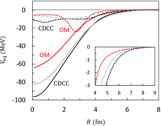
In order to analyze the CDCC results, I show in Fig. 9(d) (logarithmic scale) the Rutherford cross section, and the cross section computed with the optical potential of Ref. Kanungo et al. 2015. Surprisingly the experimental data are close to a pure Rutherford scattering. The optical potential of Ref. Kanungo et al. 2015 nicely reproduces the data. This potential is compared to the CDCC equivalent potential in Fig. 10. The main difference between them is that the CDCC predicts a larger range for the real and imaginary parts. In the single-channel approximation (grey lines), the range of the imaginary part is slightly smaller than in the full calculation. In a reaction involving two fragile nuclei, it seems natural that their interaction extends to large distances. However the optical potential which fits the data is characterized by a fairly short range. This apparent contradiction certainly deserves more experimental studies, in particular at other scattering energies.
VI Conclusion
The main goal of this work is the simultaneous investigation of and scattering at low energies. and the deuteron have a low breakup threshold, which makes the continuum quite important. In both reactions, I have used the same three-body model for . I paid a special attention to E1 transitions and I extended a previous calculation of the E1 distribution Pinilla et al. 2012 by considering a correction to the long-wavelength approximation. This correction could give rise to isoscalar E1 transitions, as suggested in Refs. Tanaka et al. 2017; Kanungo et al. 2015 on the basis of a large radius. However, if I confirm the existence of a dipole resonance at low energies, the isoscalar part of the E1 matrix element is negligible, owing to the low photon energies.
For the elastic scattering, the CDCC calculation reproduces the experiment fairly well. The role of the continuum can been seen at large angles , small angles being weakly sensitive. Notice that the calculations depend on a potential, which is available from global parametrizations only. Experimental data on elastic scattering would be helpful to derive a more accurate optical potential.
From the CDCC formalism, I have determined and equivalent potentials. The goal is to use them in scattering with the additional deuteron breakup. The comparison of these equivalent potentials with the global potential of Ref. Koning and Delaroche 2003 shows that the main difference is in the range. This result is not surprising since the large radius of , as well as its low binding energy, are not considered in global parametrizations.
The theoretical description of is a difficult challenge. The incident energy of is almost the same as in (55.3 MeV) and the c.m. energy is therefore almost double. In spite of this, the data are compatible with a pure Rutherford scattering, as shown in Fig. 9(d). I have investigated the system in two ways: in the former, I use a standard three-body model using and interactions, and in the latter I extend the CDCC formalism to five bodies, with described as . Both approaches provide qualitatively similar cross sections. At small angles , the apparent peak in the data is present in the calculation, but its amplitude is much larger. Increasing the number of pseudostates reduces the amplitude, but it remains overestimated.
The five-body calculation is a numerical challenge, owing to the very large number of channels. It is difficult to get a perfect convergence although my calculation should not be far from convergence. Of course such calculations have shortcomings: (i) the and optical potentials are not experimentally known, (ii) antisymmetrization effects between the neutrons of and of the deuteron are neglected, (iii) at these low energies, the and Pauli forbidden states may play a role.
On the experimental side, data so close to Rutherford scattering are unexpected. The authors of Ref. Kanungo et al. 2015 fit these data with an optical potential presenting a short range. This is illustrated in Fig. 10, where I compare the CDCC equivalent potential with the optical model of Ref. Kanungo et al. 2015. As for scattering, more data on , especially at small angles, would be welcome to confirm the short-range of the potentials.
Acknowledgments
I am grateful to R. Kanungo for useful discussions about the experimental data. This work was supported by the Fonds de la Recherche Scientifique - FNRS under Grant Numbers 4.45.10.08 and J.0049.19. It benefited from computational resources made available on the Tier-1 supercomputer of the Fédération Wallonie-Bruxelles, infrastructure funded by the Walloon Region under the grant agreement No. 1117545.
Appendix A Calculation of the coupling potentials
The calculation of the coupling potentials (22) is briefly presented in this Appendix. I consider systems made of a three-body projectile and, either of a structureless target (referred to as ), or of a two-body target (referred to as ). Calculations associated with 2+2 systems have been described in Ref. Descouvemont 2018.
The matrix elements (22) involve 3 or 6 terms for 3+1 and 3+2 systems, respectively. I consider one of this potentials, , associated with the Jacobi coordinates of Fig. 2. Consequently I consider for 3+1 systems and for 3+2 systems. Coefficients and are related to the masses of the fragments. This potential is expanded in multipoles: for 3+1 systems, I have
| (25) |
whereas 3+2 potentials are expanded as
| (26) |
In these expansions, I assume that the axis is along the direction. The multipole components and can be computed by numerical integration of the potentials over the angles.
Then, inserting expansion (25) in the coupling potentials (22) provide, for 3+1 systems
| (27) |
where coefficients are given by
| (28) |
and are common to all CDCC calculations, independently of the projectile and target descriptions (in the case of a structureless target the channel spin is ). I use the notation .
Coefficients are typical of 3+1 systems and are defined as
| (29) |
where the condition arises from the choice of the Jacobi coordinates. Functions are also associated with 3+1 systems; they are given by
| (30) |
where are functions depending on the hyperangle (see Refs. Descouvemont and Baye 2010; Descouvemont 2018 for more information). In this expression, the quadrature over the hyperangle is performed numerically. The hyperradial functions are expanded over Lagrange functions, and the integration over is therefore straightforward.
Equation (27) is associated to a specific term () of the total potential . I compute the matrix elements of and by using other choices of the Jacobi coordinates. The corresponding coupling potentials are therefore computed with (27) followed by a transformation using the Raynal-Revai coefficients Raynal and Revai 1970. This method was already adopted in Refs. Rodríguez-Gallardo et al. 2008; Descouvemont et al. 2015.
The extension of 3+2 systems is new. It can be extended from the previous equation in a systematic way. In that case, the target has a two-body structure and its wave function is given by (). The coupling potentials (27) are generalized as
| (31) |
where coefficients are given by
| (32) |
The functions are now defined as
| (33) |
which means that an additional integration over is required. Again, the two-body radial functions are expanded over a Lagrange mesh, and the associated quadrature is simple. As for 3+1 systems, the use of Raynal-Revai coefficients permits a similar calculation for the other components of the potential , and . An extension to 3+3 systems is feasible by adopting the same technique, and by using a double Raynal-Revai transformation.
References
- Tanihata et al. (1985) I. Tanihata, H. Hamagaki, O. Hashimoto, Y. Shida, N. Yoshikawa, K. Sugimoto, O. Yamakawa, T. Kobayashi, and N. Takahashi, Phys. Rev. Lett. 55, 2676 (1985).
- Tanihata et al. (2013) I. Tanihata, H. Savajols, and R. Kanungo, Prog. Part. Nucl. Phys. 68, 215 (2013).
- Suzuki et al. (2003) Y. Suzuki, R. G. Lovas, K. Yabana, and K. Varga, Structure and Reactions of Light Exotic Nuclei (Taylor & Francis, London, 2003).
- Rawitscher (1974) G. H. Rawitscher, Phys. Rev. C 9, 2210 (1974).
- Austern et al. (1987) N. Austern, Y. Iseri, M. Kamimura, M. Kawai, G. Rawitscher, and M. Yahiro, Phys. Rep. 154, 125 (1987).
- Di Pietro et al. (2012) A. Di Pietro, V. Scuderi, A. M. Moro, L. Acosta, F. Amorini, M. J. G. Borge, P. Figuera, M. Fisichella, L. M. Fraile, J. Gomez-Camacho, H. Jeppesen, M. Lattuada, I. Martel, M. Milin, A. Musumarra, M. Papa, M. G. Pellegriti, F. Perez-Bernal, R. Raabe, G. Randisi, F. Rizzo, G. Scalia, O. Tengblad, D. Torresi, A. M. Vidal, D. Voulot, F. Wenander, and M. Zadro, Phys. Rev. C 85, 054607 (2012).
- Matsumoto et al. (2004) T. Matsumoto, E. Hiyama, K. Ogata, Y. Iseri, M. Kamimura, S. Chiba, and M. Yahiro, Phys. Rev. C 70, 061601 (2004).
- Descouvemont (2018) P. Descouvemont, Phys. Rev. C 97, 064607 (2018).
- Tanaka et al. (2017) J. Tanaka, R. Kanungo, M. Alcorta, N. Aoi, H. Bidaman, C. Burbadge, G. Christian, S. Cruz, B. Davids, A. D. Varela, J. Even, G. Hackman, M. N. Harakeh, J. Henderson, S. Ishimoto, S. Kaur, M. Keefe, R. Krücken, K. Leach, J. Lighthall, E. P. Rodal, J. S. Randhawa, P. Ruotsalainen, A. Sanetullaev, J. K. Smith, O. Workman, and I. Tanihata, Phys. Lett. B 774, 268 (2017).
- Kanungo et al. (2015) R. Kanungo, A. Sanetullaev, J. Tanaka, S. Ishimoto, G. Hagen, T. Myo, T. Suzuki, C. Andreoiu, P. Bender, A. A. Chen, B. Davids, J. Fallis, J. P. Fortin, N. Galinski, A. T. Gallant, P. E. Garrett, G. Hackman, B. Hadinia, G. Jansen, M. Keefe, R. Krücken, J. Lighthall, E. McNeice, D. Miller, T. Otsuka, J. Purcell, J. S. Randhawa, T. Roger, A. Rojas, H. Savajols, A. Shotter, I. Tanihata, I. J. Thompson, C. Unsworth, P. Voss, and Z. Wang, Phys. Rev. Lett. 114, 192502 (2015).
- Matsumoto et al. (2019) T. Matsumoto, J. Tanaka, and K. Ogata, Prog. Theor. Exp. Phys. 2019 (2019), 10.1093/ptep/ptz126.
- Zhukov et al. (1993) M. V. Zhukov, B. V. Danilin, D. V. Fedorov, J. M. Bang, I. J. Thompson, and J. S. Vaagen, Phys. Rep. 231, 151 (1993).
- Descouvemont et al. (2006) P. Descouvemont, E. M. Tursunov, and D. Baye, Nucl. Phys. A 765, 370 (2006).
- Raynal and Revai (1970) J. Raynal and J. Revai, Nuovo Cim. A 39, 612 (1970).
- Descouvemont et al. (2003) P. Descouvemont, C. Daniel, and D. Baye, Phys. Rev. C 67, 044309 (2003).
- Baye (2015) D. Baye, Phys. Rep. 565, 1 (2015).
- Pinilla et al. (2012) E. C. Pinilla, P. Descouvemont, and D. Baye, Phys. Rev. C 85, 054610 (2012).
- Descouvemont et al. (2015) P. Descouvemont, T. Druet, L. F. Canto, and M. S. Hussein, Phys. Rev. C 91, 024606 (2015).
- Thompson et al. (1977) D. R. Thompson, M. LeMere, and Y. C. Tang, Nucl. Phys. A 286, 53 (1977).
- Esbensen et al. (1997) H. Esbensen, G. F. Bertsch, and K. Hencken, Phys. Rev. C 56, 3054 (1997).
- Baye (1987) D. Baye, Phys. Rev. Lett. 58, 2738 (1987).
- Bachelet et al. (2008) C. Bachelet, G. Audi, C. Gaulard, C. Guénaut, F. Herfurth, D. Lunney, M. de Saint Simon, and C. Thibault, Phys. Rev. Lett. 100, 182501 (2008).
- Egelhof et al. (2002) P. Egelhof, G. Alkhazov, M. Andronenko, A. Bauchet, A. Dobrovolsky, S. Fritz, G. Gavrilov, H. Geissel, C. Gross, A. Khanzadeev, G. Korolev, G. Kraus, A. Lobodenko, G. Münzenberg, M. Mutterer, S. Neumaier, T. Schäfer, C. Scheidenberger, D. Seliverstov, N. Timofeev, A. Vorobyov, and V. Yatsoura, Eur. Phys. J. A 15, 27 (2002).
- Tanihata et al. (1988) I. Tanihata, T. Kobayashi, O. Yamakawa, S. Shimoura, K. Ekuni, K. Sugimoto, N. Takahashi, T. Shimoda, and H. Sato, Phys. Lett. B 206, 592 (1988).
- Descouvemont and Baye (1987) P. Descouvemont and D. Baye, Phys. Rev. C 36, 1249 (1987).
- Nakamura et al. (2006) T. Nakamura, A. M. Vinodkumar, T. Sugimoto, N. Aoi, H. Baba, D. Bazin, N. Fukuda, T. Gomi, H. Hasegawa, N. Imai, M. Ishihara, T. Kobayashi, Y. Kondo, T. Kubo, M. Miura, T. Motobayashi, H. Otsu, A. Saito, H. Sakurai, S. Shimoura, K. Watanabe, Y. X. Watanabe, T. Yakushiji, Y. Yanagisawa, and K. Yoneda, Phys. Rev. Lett. 96, 252502 (2006).
- Lafferty Jr and Cotanch (1982) J. M. Lafferty Jr and S. R. Cotanch, Nucl. Phys. A 373, 363 (1982).
- Yahiro et al. (2012) M. Yahiro, K. Ogata, T. Matsumoto, and K. Minomo, Prog. Theor. Exp. Phys. 2012, 01A206 (2012).
- Kamimura et al. (1986) M. Kamimura, M. Yahiro, Y. Iseri, S. Sakuragi, H. Kameyama, and M. Kawai, Prog. Theor. Phys. Suppl. 89, 1 (1986).
- Descouvemont (2017) P. Descouvemont, Phys. Lett. B 772, 1 (2017).
- Druet et al. (2010) T. Druet, D. Baye, P. Descouvemont, and J.-M. Sparenberg, Nucl. Phys. A 845, 88 (2010).
- Descouvemont and Baye (2010) P. Descouvemont and D. Baye, Rep. Prog. Phys. 73, 036301 (2010).
- Descouvemont (2016) P. Descouvemont, Comput. Phys. Commun. 200, 199 (2016).
- Koning and Delaroche (2003) A. J. Koning and J. P. Delaroche, Nucl. Phys. A 713, 231 (2003).
- Varner et al. (1991) R. L. Varner, W. J. Thompson, T. L. McAbee, E. J. Ludwig, and T. B. Clegg, Phys. Rep. 201, 57 (1991).
- Ogata and Yoshida (2016) K. Ogata and K. Yoshida, Phys. Rev. C 94, 051603 (2016).
- Thompson et al. (1989) I. Thompson, M. Nagarajan, J. Lilley, and M. Smithson, Nucl. Phys. A 505, 84 (1989).
- Rodríguez-Gallardo et al. (2008) M. Rodríguez-Gallardo, J. M. Arias, J. Gómez-Camacho, R. C. Johnson, A. M. Moro, I. J. Thompson, and J. A. Tostevin, Phys. Rev. C 77, 064609 (2008).