Dynamical systems on Hypergraphs.
Abstract
Networks are a widely used and efficient paradigm to model real-world systems where basic units interact pairwise. Many body interactions are often at play, and cannot be modelled by resorting to binary exchanges. In this work, we consider a general class of dynamical systems anchored on hypergraphs. Hyperedges of arbitrary size ideally encircle individual units so as to account for multiple, simultaneous interactions. These latter are mediated by a combinatorial Laplacian, that is here introduced and characterised. The formalism of the Master Stability Function is adapted to the present setting. Turing patterns and the synchronisation of non linear (regular and chaotic) oscillators are studied, for a general class of systems evolving on hypergraphs. The response to externally imposed perturbations bears the imprint of the higher order nature of the interactions.
I Introduction.
Network science Albert and Barabási 2002; Boccaletti et al. 2006 has proved successful in describing many real-world systems Newman 2010; Barabási et al. 2016; Latora et al. 2017, which, despite inherent differences, share common structural features. Even more interestingly, dynamical processes and hosting networks are indissolubly entangled with the ensuing patterns that reflect in fact the complex topology of the supports to which they are anchored Castellano et al. 2009; Arenas et al. 2008; Barrat et al. 2001.
Networks constitute abstract frameworks, where pairwise interactions among generic agents, represented by nodes, are schematised by edges. Stated simply, two agents are connected if they interact. Hence by their very first definition, networks encode for binary relationships among units. This descriptive framework is sufficiently accurate in many cases of interest, although several examples exist of systems for which it holds true just as a first order approximation Benson et al. 2016; Lambiotte et al. 2019. The relevance of high-orders structures has been indeed emphasised in the context of functional brain networks Petri et al. 2014; Lord et al. 2016, in applications to protein interaction networks Estrada and Ross 2018, to the study of ecological communities Grilli et al. 2017 and co-authorship networks Patania et al. 2017; Carletti et al. 2020.
Starting from this observation, higher-order models have been developed so as to capture the many body interactions among interacting units. The most notable examples are simplicial complexes Devriendt and Van Mieghem 2019; Courtney and Bianconi 2016; Petri and Barrat 2018 and hypergraphs Berge 1973; Estrada and Rodríguez-Velázquez 2005; Ghoshal et al. 2009, non trivial mathematical generalisations of ordinary networks that are currently attracting a lot of interest. The concept of simplicial complexes has been for instance invoked to address problems in epidemic spreading Bodó et al. 2016; Iacopini et al. 2019 or synchronisation phenomena Lucas et al. 2020; Gambuzza et al. 2020. Our work is positioned in the framework of hypergraphs, a domain of investigation which is still in its infancy. In this respect, we mention applications to social contagion model de Arruda et al. 2020; Ferraz de Arruda et al. 2020, to the modelling of random walks Carletti et al. 2020 and to the study of synchronisation Krawiecki 2014; Mulas et al. 2020 and diffusion Ferraz de Arruda et al. 2020.
Hypergraphs constitute indeed a very flexible paradigm: an arbitrary number of agents are allowed to interact, thus extending beyond the limit of binary interactions of conventional network models. On the other hand, hypergraphs define a leap forward as compared to simplicial complexes. In this latter case, in fact, if (say) agents form a -simplex, also all binary interactions are accounted for. On the other hand, agents interacting via a hypergraph do form a hyperedge, a unifying frame which encompasses the many body interactions as a whole. Imagine that a subgroup of agents organised in the hyperedge, also interact with each other via a distinct channel; this yields a new hyperedge, included in the former. A hypergraph can reproduce, in a proper limit, a simplicial complex and, in this respect, provides a more general tool for addressing many body simultaneous interactions.
Furthermore, the analysis of the models in the framework of hypergraphs turns out to be simpler as compared to their simplicial complexes homologues. In these latter settings, the involved formulas get rapidly cumbersome and, for this reason, applications are limited to low dimensional simplexes, i.e. or -simplex. At variance, one can efficiently handle very large hyperedges and, even more importantly, heterogenous distribution of hyperedges’ sizes, because all the information on the high-order structure of the embedding support are stored in a matrix whose dimension depends only on the number of nodes Carletti et al. 2020; Ferraz de Arruda et al. 2020.
Starting on these premises, it is clear that many body interactions constitute a relevant and transversal research field that is still in its embryonic stage, in particular as concerns studies that relate to hypergraphs. Indeed, novel light could be shed on a large plethora of systems, usually defined on standard networks, by accounting for generalised hypergraph architectures. This paper aims at taking one first step in this direction, by expanding along different axis. We will begin by adapting to the hypergraph setting the Master Stability Function Pecora and Carroll 1998 formalism. We will then consider the condition for the emergence of Turing patterns Turing 1952 for reaction-diffusion systems on hypergraphs, the synchronisation of nonlinear oscillators Arenas et al. 2008 and of chaotic orbits. It is here anticipated that for theoretical progress to be made one needs to characterise the spectral properties of a properly defined operator, which implements diffusion on hypergraphs.
The Master Stability Function (MSF), is a powerful technique developed in Pecora and Carroll 1998 to analyse synchronisation and it basically amounts to performing a linear stability analysis around a given equilibrium orbit, for a system of coupled interacting units. A straightforward application of linear stability analysis is for instance found in the context of the celebrated Turing instability, once the reference orbit is indeed a homogeneous fixed point.
In his seminal paper Turing 1952, Alan Turing set the mathematical basis of pattern formation. Initially proposed to explain the richness and diversity of forms displayed in Nature, the theory elaborated by Turing is nowadays an universally accepted paradigm of self-organisation Ball 1999; Nicolis and Prigogine 1977; Murray 2001. The onset of pattern originates from the loss of stability of an homogeneous equilibrium, as triggered by diffusion. Turing instabilities have been initially studied for systems defined on continuous spatial domains and regular lattices Othmer and Scriven 1971. More recently, the realm of application of Turing ideas has been extended to account for reaction-diffusion dynamics hosted on a complex network Nakao and Mikhailov 2010 and other related structures, such as multilayer networks Asllani et al. 2014; Kouvaris et al. 2015 or multigraphs Asllani et al. 2016 just to mention a few. It is hence a natural question to generalise these studies to the broad framework of hypergraphs.
Turing patterns emerge from the destabilisation of a homogeneous equilibrium, that is a stationary solution of the examined model. In many real cases, however the system is not bound to evolve close to a stationary solution, but instead displays periodic oscillations. Examples ranges from biology to ecology, passing through physics Pikovsky et al. 2001; Arenas et al. 2008: individual nonlinear oscillators can synchronise and thus exhibit a coherent collective behaviour. Synchronisation, the spontaneous ability of coupled oscillators to operate in unison, has been studied for systems interacting via a complex and heterogeneous network of interlaced connections. To the best of our knowledge, however, this analysis has never been attempted for systems defined on hypergraphs of the type here considered. Let us observe that, although similar in their conception, the works Sorrentino 2012; Bilal and Ramaswamy 2014 deal with hypernetworks, namely a network where several different links can connect two nodes, also called multigraph in the literature. The interactions are hence pairwise.
The formalism of the MSF can be also applied to chaotic oscillators. The synchronisation of chaotic systems defined on hypergraphs has been studied in Krawiecki 2014 by using the formalism of the MSF under two main assumptions: (i) the work has been limited to -hypergraphs, namely assuming that all the hyperedges have the same size ; (ii) the coupling function was assumed to be invariant with respect to permutations of the nodes, within each hyperedge. In this paper, we will relax both assumptions to deal with general hypergraphs with heterogenous hyperedge size distribution and without putting forward any hypothesis on the form of the coupling function.
In a recent work Mulas et al. 2020, the synchronisation phenomenon has been studied resorting again to the MSF, but employing however a Laplace operator Jost and Mulas 2019 which cannot account in full for the high order interaction at play. The employed operator is defined from the hyper-adjacency matrix, which is solely capable to encode for the number of incident hyperedges without gauging their sizes. Moreover authors assumed the coupling function to depend on the average (arithmetic or geometric) value of the involved variables. Again, both assumptions are relaxed in the present work, because our Laplace operator takes into account both the number of incident hyperedges but also their size. We will moreover make use of a generic coupling function.
The paper is organised as follows. We first review the formalism of hypergraphs and introduce a new combinatorial Laplace matrix for hypergraphs. We then turn to discussing the spectra of the newly introduced Laplacian by emphasising its localisation properties. Then we present three applications, following the logic path outlined above, and elaborate on the impact of high-order structures. We finally conclude and sum up of our results.
II Hypergraphs.
Let us consider an hypergraph , where denotes the set of nodes and the set of hyperedges, that is for all : , i.e. an unordered collections of vertices. Note that if , i.e. , then the hyperedge is actually a “standard” edge denoting a binary interaction among and . If all hyperedges have size then the hypergraph is actually a network. If an hyperedge contains all its subsets, then we recover a simplicial complex.
We can define the incidence matrix of the hypergraph 11 1 We will adopt the convention of using roman indexes for nodes and greek ones for edges., , which carries information on how nodes are shared among edges (see middle panel Fig. 1). More precisely
| (1) |
With such a matrix one can construct the adjacency matrix of the hypergraph, , whose entry represents the number of hyperedges containing both nodes and . Note that often the adjacency matrix is defined by setting to the main diagonal. Let us also define the hyperedges matrix , whose entry counts the number of nodes in .
The adjacency matrix of the hypergraph allows one to define a Laplace matrix Jost and Mulas 2019; Mulas et al. 2020, whose entries are given by , where denotes the number of hyperedges incident with node . This matrix generalises the (combinatorial) Laplace matrix for networks. However it does not account in full for the higher-order structures encoded in the hypergraph. Notably, the sizes of the incident hyperedges are neglected.
To overcome this limitation, authors of Carletti et al. 2020 studied a random walk process defined on a generic hypergraph using a new (random walk) Laplace matrix. It is worth mentioning that the transition rates of the associated process, linearly correlates with the size of the involved hyperedges. Stated differently, exchanges are favoured among nodes belonging to the same hyperedge (weighted according to its associated size). This allows in turn to describe the tightness of high-order interactions among “close nodes”. More precisely:
where the entries of are given by
| (2) |
and is a matrix whose diagonal coincides with that of and it is zero otherwise.
From this random walk Laplace operator, one can straightforwardly derive the (combinatorial) Laplace matrix,
| (3) |
that will be employed in this paper to investigate the effect of diffusion on higher-order structures. In the above equation, matrix contains on the diagonal the values and zeros otherwise. It is clear from its very definition that takes into account both the number and the size of the hyperedges incident with the nodes. It can also be noted that can be considered as a weighted adjacency matrix whose weights have been self-consistently defined to account for the higher-order structures encoded in the hypergraph (see right panel of Fig. 1).
It is worth emphasising that the dynamics defined on this weighted network is equivalent Chitra and Raphael 2019 to the dynamics on the corresponding hypergraph. This observation allows us to transport existing tools targeted to networks’ analysis to the realm where nodes are made to interact via hypergraphs. In particular, studying linear dynamical systems evolving on a hypergraph amounts to operating with standard matrices, where stands for the number of nodes. In this respect, the analysis is straightforward, and avoid the complications that are to be faced when dealing with simplicial complexes, where tensors are instead involved (see Section IV).
Given a hypergraph one can construct the projected network, that is the network obtained by mapping the nodes belonging to a hyperedge into a clique of suitable size (see left panel Fig. 1). If the hypergraph contains only simple hyperedges, then this projection is invertible and, given a network, one can construct a unique hypergraph whose projection coincides with the network itself Carletti et al. 2020. Let us observe that the projected network keeps track of the many body interactions only though the cliques, i.e. relying on binary exchanges.
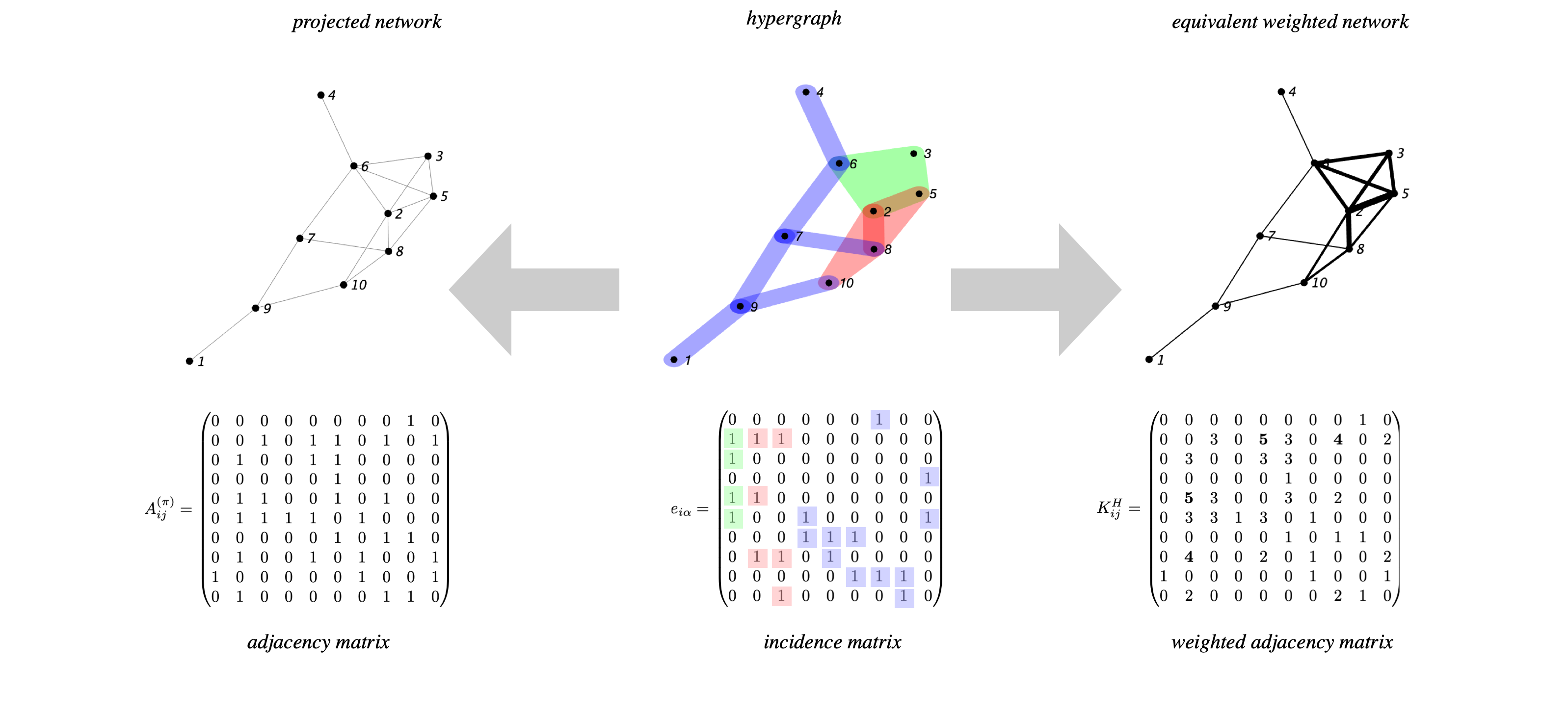
Let us conclude this section by remarking that the operator , given by Eq. (3), admits as eigenvector associated to the zero eigenvalue. This latter homogeneous solution can be stable, so resilient, to external perturbation for a system evolving on a hypergraph and subject to nonlinear reaction terms. Instabilities can alternatively develop, depending on the specific explored setting. These issues will be addressed in the following by assuming higher-order interactions encoded by the hypergraph, to link co-evolving populations. Inspecting the stability of this generalised class of reaction-diffusion systems, amounts to studying the spectra of the coupling operator. For this reason we shall begin hereafter by analysing the spectra of a hypergraph Laplacian.
III Localisation of eigenvectors
One can prove Carletti et al. 2020 that is symmetric, non-negatively defined and its largest eigenvalue equals . Moreover, let be the set of its eigenvalues of , then , and its eigenvectors, form an orthonormal basis, . As already observed, . Finally reduces to the Laplace matrix defined on networks once all the hyperedges have size . In the following we will denote by the eigenvalues of the Laplace operator of the projected network, , and the associated eigenvectors. Based on the well known properties of and assuming the network to be connected, we have and the eigenvectors do form an orthonormal basis.
Localisation of eigenmodes is a phenomenon relevant to many fields of science, e.g. the Anderson localisation in disordered systems Anderson 1958; Grebenkov and Nguyen 2013, with a particular relevance to dynamics. For this reason we decided to start our analysis by studying the localisation properties of the Laplacian eigenvectors for the hypergraph (3) and compare them with the corresponding quantities obtained for the projected network. Results reported in Fig. 2 show that the localisation is more evident for a hypergraph, than for the associated projected network. In the left panel of Fig. 2, we present the eigenvectors for the Laplace matrix stemming from the hypergraph (ordered for increasing eigenvalue ) as a function of the nodes indexes (ordered for increasing ). In the right panel, the same quantity is displayed for the Laplace matrix computed from the projected network. In this latter case, the nodes are ordered for increasing degree. By visual inspection (entries larger than are coloured in black while the remaining ones are drawn in white), one can clearly appreciate the dark squarish zones, associated to small or medium rank eigenvectors, which appear in the left panel of Fig. 2: eigenvectors are found with relatively large entries across many nodes, i.e. a strong localisation. On the right panel, similar structures are present but much weaker. A substantially analogous behaviour is observed for high ranked eigenvectors, e.g. in the left panel and in the right one, for which only few entries display very large values, pointing hence to an even stronger localisation (see the thin dark “line” in the top right corners in both panels).
To illustrate our results, we employed as projected network a Scale Free network made by nodes, built by using the configuration model with and Latora et al. 2017. The associated hypergraph is obtained by transforming all the maximal -cliques into hyperedges of size . The distribution of hyperedges sizes is reported in Fig. 3.


A more quantitative measure of the localisation, can be obtained by using the Inverse Participation Ratio (IPR) McGraw and Menzinger 2008. For a -dimensional vector, , this is defined as
| (4) |
The above quantity ranges in , where the lower bound is attained for a vector with uniform entries. The upper limit is hit when all entries are but one, which equals . In Fig. 4 we report the IPR computed for the eigenvectors of the hypergraph (blue dots) and the projected network (black dots) used in Fig. 2. We can observe that in the case of the hypergraph, the IPR is always larger than the homologous quantity computed for the projected network, except for very high ranked eigenvectors (say, the last ones).
In the next section we will show that the localisation which manifests on hypergraph, leaves macroscopic imprints on the dynamics of systems subject to many-body, higher-order interactions. This issue will be discussed in the following Section.
IV Dynamical systems on hypergraphs
In the remaining part of this paper we will consider the behaviour of dynamical systems defined on hypergraphs. In particular, we will analyse the consequences of dealing with higher-order couplings, exploiting to this end the spectral characteristics highlighted above. More specifically, assume copies of the same low dimensional dynamical system to be hosted on each node of a given collection. This defines the local dynamics of the inspected system. Units belonging to different nodes are assumed to interact through higher-order structures identified as hyperedges. Many body interactions promote a preferential interaction among nodes belonging to the same large hyperedge. The nodes can be imagined to identify different spatial locations. For this reason we will denote by aspatial the system composed by one isolated dynamical unit, and use spatial to refer to its multi-dimensional version made of mutually entangled components.
As already mentioned the newly introduced (combinatorial) Laplace matrix (3) admits a homogeneous eigenvector associated to the zero eigenvalue. This will allow us to probe (in)stability of interconnected systems evolving close to reference orbits. For the sake of completeness, we will consider three distinct applications that cover several relevant research domains. We will begin by imposing a generalised diffusive coupling among nodes as exemplified by the aforementioned Laplace matrix (3). Working in this framework, we will study the emergence of Turing patterns, that is the conditions that promote the emergence of a stable heterogeneous solution. We will then turn to considering the synchronisation between nonlinear oscillators, diffusively coupled via higher-order combinatorial Laplacians. Finally, we will analyse the synchronisation of chaotic oscillators, in the setting of interest where higher-order interactions are at play. The formalism of the Master Stability Function, will be used to tackle the problem analytically. Projected networks will be employed as reference benchmarks to bring into evidence the role of hypergraphs and related higher order interactions.
Consider a -dimensional system described by local, i.e. aspatial, equations:
| (5) |
and fix a reference orbit, . Let us observe that the latter can also be a fixed point. Assume further identical copies of the above system coupled through a hypergraph, namely each copy is attached to a node of a hypergraph. Moreover, each unit belongs to one (or more) hyperedge. Units sharing the same hyperedge are tightly coupled, due to existing many body interactions. In formulas:
where denotes the state of the -th unit, i.e. anchored to the -th node, the strength of the coupling and a generic nonlinear coupling function. The elements of matrix denote the size of the hyperedge . The factor account for the fact that should be different from . Recalling the definition of one can rewrite the previous formula as
| (6) | |||||
where we have used the definition of and given by (3). Let us stress once again that all the high-order structure is encoded in a matrix and there is no need for tensors as in the case of simplicial complexes: this simplifies the resulting analysis.
By exploiting the fact that for all , it is immediate to conclude that the aspatial reference solution is also a solution of Eq. (6). A natural question that arises is hence to study the stability of the homogeneous solution for the system in its coupled variant.
To answer to this question one introduce the deviations from the reference orbit, i.e. . Assuming this latter to be small, one can derive a self-consistent set of linear equations for tracking the evolution of the perturbation in time. To this end, we make use of the above expression in Eq. (6) and perform a Taylor expansion by neglecting terms of order larger than two, to eventually get:
| (7) |
where (resp. ) denotes the Jacobian matrix of the function (resp. ) evaluated on the trajectory .
Remember that is symmetric. Hence, there exists a basis formed by orthonormal eigenvectors, , associated to eigenvalues (see Section III). We can then project on this basis and obtains for all :
| (8) |
where is the projection of on the -th eigendirection.
Let us finally conclude this section by observing that from Eq. (8) one can derive the Master Stability Function, i.e. the most general framework to address questions that pertain to the stability of the reference orbit. Despite its generality, the latter can only be handled numerically, except very few exceptions. In the following we begin by studying the setting where is a constant solution. In this case the Eq. (8) simplifies because the right hand side is no longer time dependent and the problem reduces to a classical study of Turing instability. Indeed, the rightmost term in Eq. (6) can be seen as a sort of generalised Fickean diffusion (see Section IV.1). If the reference orbit is instead periodic in time, one can investigate the conditions which drive the synchronisation of regular oscillators. In this case the Master Stability Function can be analysed by resorting to the Floquet machinery. In the following, we have however chosen to study the synchronisation of Stuart-Landau oscillators via higher-order couplings (see Section IV.2). Working in this setting, the Master Stability Function becomes again time independent and the analysis closely resembles the one carried out for addressing the onset of Turing instabilities. As a final step, we will turn to studying the case where is a chaotic trajectory (see Section IV.3).
IV.1 Turing patterns on hypergraphs
The Turing instability takes place for spatially extended systems: a stable homogeneous equilibrium becomes unstable upon injection of a heterogeneous, i.e. spatially dependent, perturbation once diffusion and reaction terms are simultaneously at play. Let us first consider two generic nonlinear functions and describing the local dynamics
| (9) |
Then assume to replicate such system on all the nodes of a given hypergraphs, and label and the corresponding concentration. Here the index refers to the specific node to which the dynamical variables are bound. Finally, assume that two nodes, and , communicate if they belong to the same hyperedge and moreover the strength of the interaction (which results in an effective transport across the involved nodes) is mediated by both the number of shared hyperedges and their sizes. Indeed, nodes belonging to the same hyperedge exhibit a higher-order interaction and we consequently assume that spreading among them is more probable than with nodes associated with other hyperedges or smaller ones. From a microscopic point of view, imagine to deal with a walker belonging to a given node. The walker assigns to all its neighbours a weight that gauges the size of the hyperedges and the number of incident hyperedges, and then she performs a jump with a probability proportional to this weight. This represents a higher-order extension Ficks’ law: the rate of change of is proportional to
where use has been made of matrix , as introduced above. Recalling the definition of one can rewrite the previous formula as
where we have used the definition of and .
So in conclusion a reaction-diffusion processes on hypergraphs, where the diffusion takes into account the higher-order interactions among nodes in the same hyperedge, can be described by the following system
| (10) |
where and are effective diffusion coefficients of species and . At first sight, the above model seems to solely account for binary interactions. However, higher-order interactions are also present, as encoded in the matrix . This is thus a compact formalism allowing to overcome the computational issues intrinsic to simplicial complexes. Finally, let us observe that if the hypergraph is a network, i.e. the hyperedges have size , , then reduces to the standard Laplace matrix. Thus Eqs. (10) converges to the standard reaction-diffusion system defined on a network.
The condition for the emergence of a Turing instability can be detected by performing a linear stability analysis about the homogeneous equilibrium. More precisely, the latter is assumed to be stable with respect to homogeneous perturbations, while it loses its stability for heterogeneous perturbations once diffusion is at play, and . The linear stability analysis can be performed by following the standard procedure: (i) by linearising the model (10) around the equilibrium, for all ; (ii) by expanding the perturbations on the eigenbasis of , and (iii) by calculating the dispersion relation, i.e. the linear growth rate of the eigenmode , as a function of the Laplacian eigenvalue . The linear growth rate is the real part of the largest root of the second order equation
| (11) |
where is the Jacobian matrix of the reaction part evaluated at the equilibrium , (resp. ) is its trace (resp. determinant). The concept of dispersion relation is close to that of Lyapunov exponent: the existence of eigenvalues for which the dispersion relation takes positive values, implies that the system goes unstable via a typical path first identified by Alan Turing in his seminal work. At variance, if the dispersion relation is negative the system cannot undergo a Turing instability: any tiny perturbation fades away and the system settles back to the homogeneous equilibrium.
To provide a concrete example, we assume the reaction kinetic to be modelled by the Brusselator scheme Prigogine and Nicolis 1967; Prigogine and Lefever 1968. This is a nonlinear model defined by and , where and act as tunable parameters. We first show an example of Turing pattern emerging in both the hypergraph and its related projected network (the same used in the previous section). In the main panels of Fig. 5 the dispersion relations are reported: a subset of eigenvalues exist which is associated to positive values of the dispersion relation, for both the hypergraph –panel (a)– and the projected network –panel (b). In the insets of Fig. 5 we display the ensuing patterns. Nodes are ordered for increasing hyper degree (resp. degree) for the hypergraph (resp. the projected network). One can clearly observe that, in the case of the hypergraph, patterns are strongly localised in nodes associated to larger hyper degree.

From Fig. 5 one can also observe that the domain of definition of the eigenvalues for the hypergraph cover a much wider range, as compared to that associated to the projected network. This observation can open the way to settings where patterns emerge only for systems defined on top of hypergraphs and not on the corresponding projected networks. In this case, patterns are the result of the higher-order interaction among nodes. To challenge this scenario, let us consider a small network built by using the Barabási-Albert algorithm Albert and Barabási 2002 with nodes. For each iteration of the generative algorithm, new nodes are attached to the already existing ones, according to a preferential attachment scheme; because of the small size of the network, our goal here is not to resolve the scale free nature of the network but to obtain a hierarchical structure where -cliques, and larger ones, are mutually connected. We identify the complete cliques and build the associated hypergraph by assuming each -clique to form a hyperedge with size . We then turn to considering the resulting hypergraph and the associated projected network as the underlying support for the dynamics (10). The dispersion relation can be computed (see main panels of Fig. 6): observe that the homogenous equilibrium is stable even in presence of diffusion on the network while it looses stability in the case of the hypergraph. In this latter setting Turing patterns are hence expected to develop. This can be checked by computing the time evolution of the species density both on the hypergraph and the projected network. By inspection of Fig. 6 one can appreciate that heterogenous patterns develop in the former case (see inset in the panel (a) of Fig. 6). Patterns are instead lacking in the latter scenario, i.e. when the Brussellator model hosted on the projected network (see inset in the panel (b) of Fig. 6).

IV.2 Synchronisation of Stuart-Landau oscillators on hypergraphs
In the previous section we studied the emergence of Turing patterns for reaction-diffusion systems defined on a hypergraph so as to account for many body interactions. These patterns originate from a symmetry breaking instability induced by an externally imposed perturbation acting on systems initially close to a stationary homogeneous equilibrium. In many relevant problems, systems display periodic solutions. It is therefore important to investigate the stability of isolated periodic orbits and, even more essential, to study the dynamics of extended systems which combine several replica of the same nonlinear oscillators. Imagine that individual oscillators are evolving in phase and introduce a non homogeneous perturbation. If the system is globally stable the perturbation gets eventually re-absorbed and the oscillators display a synchronous dynamics Arenas et al. 2008. Otherwise the perturbation develops in time and the system evolves towards a distinct, heterogeneous, attractor.
To study the synchronisation via a hypergraph, we consider individual units obeying to a Stuart-Landau (SL) equation Stuart and DiPrima 1978; Kuramoto 1984. This is a paradigmatic model of nonlinear oscillators, often invoked for modelling a wide range of phenomena, from nonlinear waves to second-order phase transitions, from superconductivity and superfluidity to Bose-Einstein condensation Aranson and Kramer 2002 Besides, the SL equation can be considered as a normal form for systems close to a supercritical Hopf-bifurcation. In this respect, the results here presented are more general than the specific setting explored.
Consider an ensemble made of nonlinear oscillators and label with their associated complex amplitude. Each oscillator obeys a complex Stuart-Landau equation
where is a real parameter and . Let us observe that the former admits the limit cycle solution .
We then assume the oscillators to be coupled via a many body diffusive-like interaction which can be described by the discrete Laplacian matrix (3), returning thus the system
| (12) |
where is a second real parameters and is a suitable parameter setting the coupling strength. Based on the properties of the Laplace matrix, one can prove that the limit cycle solution, , is also a solution of Eq. (12). To characterise the stability of the latter to heterogeneous perturbation, we rewrite using polar coordinates as:
| (13) |
Assuming and to be small, one can insert the (13) into Eq. (12) and then linearise the resulting equation, to get:
| (14) |
Remark that, even if we are perturbing around a limit cycle, namely a time dependent solution, the coefficients of the linearised equations do not depend on time, owing to the specific structure of the GL equation. This observation will simplify the successive analysis, which will follow closely that discussed in the preceding section for the case of a Turing instability. In the next section we will instead deal with a problem for which the linearised dynamics yields a time dependent Jacobian.
To proceed further we expand the perturbations and on the Laplacian eigenvectors basis
| (15) |
inserting the latter into (14), and by using the orthonormality of the eigenvectors, we obtain:
| (16) |
We put forward the ansatz of exponential growth for each mode, that is and and we eventually obtain a condition formally equivalent to the dispersion relation
| (17) |
Let us observe that , signifying that the reference orbit is a limit cycle and thus neutral stable. On the other hand if is positive for some , the perturbation grows exponentially in time, and the initial homogeneous state proves unstable. Conversely, if , for every , the perturbation fades away and the system converges back to the fully synchronised state. Expanding (17) for small we get
By recalling that , and for , one can conclude Cencetti et al. 2017 that for some if and only if , that is a necessary and sufficient condition for the loss of stability of the fully synchronised solution.
The numerical results reported in Fig. 7 complement the analytical theory discussed above. In panel (a) of Fig. 7 we present the dispersion relation and the heterogeneous patterns emerging for both the hypergraph and the associated projected network, for , and . The dispersion relation is positive over a finite domain and the patterns (represented by ) that develop as follow the instability are pretty localised. In panel (b) of Fig. 7, the parameters are set to the values , and . The dispersion relation is non positive and the system displays synchronised oscillations: the imposed perturbation dies out and the oscillators evolve at unison.

IV.3 Master Stability Function on hypergraphs
In the previous section we have analysed the synchronisation of an ensemble made of Stuart-Landau (SL) oscillators defined on a hypergraphs. To this end we employed a straightforward generalisation of the techniques presented in section IV.1, when investigating the emergence of Turing patterns. The use of the dispersion relation has been made possible because, for coupled SL equations, the variational problem yields a time independent Jacobian, once evaluated on the periodic homogeneous solution (14). This is not true for generic nonlinear oscillators. To overcome this problem one can however resort to the formalism of the Master Stability Function (MSF) Pecora and Carroll 1998, as introduced above. The aim of this section is thus to study the MSF in its full generality for systems defined on hypergraph. In particular, we will set to analyse the synchronisation of nonlinear chaotic oscillators coupled through a hypergraph and compare the outcome of the analysis to that obtained when operating the system on the corresponding projected network.
Let us consider again Eq. (8) and replace now in the latter equation by a generic parameter and thus also the projection by a generic “perturbation” vector
| (18) |
The largest Lyapunov exponent of Eq. (18) is called the Master Stability Function Pecora and Carroll 1998. Let us denote it by to emphasise its dependence on the parameter . If for all , , then decays to . At variance, if there exists such that , then will grow. Back to Eq. (8) one can conclude that if for a given there exists such that , then the associated grows in time. Thus individual units deviate from the reference solution . On the other hand if for all one has then the system reaches a globally synchronised state: all units will follow at the unison the same chaotic orbit. Let us observe that being the reference orbit, , a chaotic one.
To proceed in the analysis we assume linear coupling functions Huang et al. 2009: in this way the MSF simplifies, since is a constant matrix. Moreover, we will assume the matrix to have only one non zero element, say which denotes the existence of a coupling between the –th and the -th component of .
Let us observe that the variational equation still contains explicitly the time variable via the Jacobian of the reaction part, , which is indeed evaluated on the chaotic orbit. Hence to compute the MSF we have to solve a non autonomous system of ODEs, to study the evolution of the norm of and then use the definition of the maximum Lyapunov exponent . This can result in a tricky exercise. Indeed if then the norm can quickly increase to produce an overflow. On the other hand, if , then shrinks below round-off error. For this reason we employed in our analysis the Mean Exponential Growth of Nearby Orbits (MEGNO) algorithm Cincotta and Simó 2000; Cincotta et al. 2003. This is an improved chaos indicator that allows to rapidly discriminate between chaotic and regular orbits. The method makes it possible for the Lyapunov exponent to be consequently recovered. For these reasons, MEGNO has been largely used in the framework of planetary systems Goździewski et al. 2002; Libert et al. 2011, satellites and spatial debris Valk et al. 2009; Compere et al. 2012; Hubaux et al. 2013 and also generic nonlinear dynamical systems Cincotta et al. 2003. The method overcomes the above mentioned limitation by performing a sort of time average of the norm of the deviation vector (see Appendix A).
Without loss of generality we will use the Lorenz model Lorenz 1963 for a demonstrative application:
| (19) |
In the following we will fix the model parameters to the “standard values”, , and for which the system exhibits the chaotic orbit with a “butterfly shape”. Once we couple the above ODE using high-order interactions, i.e. the hypergraph, we get
| (20) |
where the constant matrix encodes for the coupling among the three variables and its entries take values or . For instance if and otherwise , (noted for short ) then the growth rate of the second variable, , depends on the first one, , that is (discarding the reaction part).
We are now in a position to adapt the above described theory, i.e. linearise about the reference orbit and project the perturbation on the eigenbase of the Laplace matrix, to Eq. (8) for the case of the Lorenz system. We will in particular compute the MSF to check the stability of the homogeneous states obtained by replicating chaotic Lorenz trajectory on each node of the collection. In the main panel of Fig. 8 we report the MSF for the coupling scheme, , that in the classification proposed in Huang et al. 2009, corresponds to class , namely the MSF is monotone decreasing and it has a single root. We consider in particular two values of the coupling strength (panel (a)) and (panel (b)). For (sufficiently) small coupling strength (panel (a)), the MSF evaluated on the discrete spectrum of the hypergraph Laplace matrix (green dots) is always negative and thus the system synchronises to the chaotic reference orbit, as shown in the inset . On the other hand the MSF for the projected network (red dots) takes positive values: the chaotic oscillators cannot synchronise, as we can appreciate from inspection of inset . For large enough coupling strength (panel (b)), both spectra yeld a negative MSF (green and red dots in panel (b)) and hence, in both cases, the systems do synchronise (see insets and ).
From these results one can draw a first conclusion. Once we fix the coupling strength , the sign of the MSF depends on the spectrum of the Laplace matrix for the hypergraph, . Similarly for the projected network. However, as we observed in Section III the eigenvalues of the hypergraph Laplacian extend over a large portion of the real axis, as compared to what it happens when considering the projected network. Hence the coupling scheme favours the synchronisation on the hypergraph, provided the coupling strength is sufficiently small. Said figuratively, one can act on the “knob” and have the spectra to slide on the MSF: by progressively reducing the value of one can force the spectrum of the projected network to enter the zone where the MSF is positive, whereas for the same value of the spectrum of the hypergraph is still associated to a negative MSF.

In Fig. 9 we report a similar analysis for the coupling schemes (a panel) and (panel (b)). In the classification proposed in Huang et al. 2009 the former corresponds the class , two zeros, while the latter to , three zeros. From the results shown in Fig. 9, one can conclude that the system behaves similarly for couplings and : if the coupling is sufficiently large (here ), synchronisation is found on the hypergraph but not on the corresponding projected network. This generalises our previous observation to all couplings belonging to an odd class .
The reported behaviour is reversed once we consider couplings that belong to an even class. As we can appreciate from inspection of Fig. 9 panel (a) one can choose a sufficiently small coupling to have the MSF negative on the projected network (red dots), while it takes positive values, when the problem formulated on the hypergraph (green dots).

V Conclusion
In this work we took a step forward in modelling dynamical systems on networks. The aim of the work is to account for high-order interactions among coupled units. In particular we focused on the hypergraphs, a very versatile setting where to model systems endowed with many-body interactions. Indeed one can easily represent such high-order interactions via the hyperedge, so as to overcome the limitations intrinsic to dealing with binary exchanges.
Starting from a microscopic process which takes place on the hypergraph, i.e. a random walk biases toward the size and the number of hyperedges a node belongs to, we defined a new combinatorial Laplace operator which generalises the concept of diffusive interaction to a multidimensional setting. This operator reduces to the standard combinatorial Laplacian once the hypergraph converges back to an ordinary network. In this respect, the newly introduced Laplacian can be rationalised as a natural extension of the usual operator.
In this framework we considered dynamical systems defined on top of hypergraphs and analysed the stability of the associated homogeneous equilibria. In particular we extended the Master Stability Function to this formalism and investigated the specificity of Turing patterns for the generalised proxy of reaction-diffusion systems on hypergraphs. We also analysed the synchronisation of periodic and chaotic orbits, shedding light on the role exerted by high-order couplings.
In all the inspected cases, the spectral properties of the novel Laplace operator are central in shaping the ensuing patterns, which appear remarkably localised, as illustrated with reference to the Turing setting. Further, hypergraphs can enhance or impede the synchronisation, as compared to what it happens on the corresponding projected network, depending on the specificity of the imposed couplings.
Appendix A Compute the MSF using MEGNO
To compute the MSF one has to solve Eq. (8). By discarding the partitioning into reaction and coupling parts, one can rewrite the previous equation as
that is a time dependent ODE, often named variational equation. The latter should thus be solved together with the evolution of the reference trajectory
where again we combine in the reaction and the coupling parts.
Then calling the solution of the variational equation with initial datum , the Mean Exponential Growth factor by Nearby Orbits (MEGNO) Cincotta and Simó 2000; Cincotta et al. 2003, can be defined as:
| (21) |
where , i.e. the norm of the vector , being the scalar product. We also emphasised that the MEGNO is being computed with respect to the reference orbit . A trivial computation gives:
| (22) | |||||
hence
| (23) |
where is the Hermitian part of .
Together with the MEGNO one usually defines also the (time)–averaged MEGNO:
| (24) |
could in principle display large oscillations for large , so limiting its effective predictive power. At variance, it can be shown that the average-MEGNO is well behaved and allows to study the dynamics for long times. Indeed the main feature of the average-MEGNO (and/or the MEGNO) is to allow to distinguish between regular orbits, for which , and irregular orbits, for which grows unbounded. More precisely, where is the largest Lyapunov characteristic number (or maximal Lyapunov exponent) of the orbit . Let us observe that for regular orbits, MEGNO is able to differentiate between periodic ones, , and quasi-periodic ones, .
Let us observe that one can overcome the problem of the growth of in case of chaotic orbits by employing the following trick. Assume to represent a solution of the variational equation. Then one can introduce the “reduced vector” , , whose evolution is given by:
It can easily proven that . Indeed
where use has been made of the fact that .
References
- Albert and Barabási (2002) R. Albert and A.-L. Barabási, Reviews of modern physics 74, 47 (2002).
- Boccaletti et al. (2006) S. Boccaletti, V. Latora, Y. Moreno, M. Chavez, and D.-U. Hwang, Physics Reports 424, 175 (2006).
- Newman (2010) M. E. Newman, Networks: An Introduction (Oxford University Press, Oxford, 2010).
- Barabási et al. (2016) A.-L. Barabási et al., Network science (Cambridge university press, 2016).
- Latora et al. (2017) V. Latora, V. Nicosia, and G. Russo, Complex networks: principles, methods and applications (Cambridge University Press, 2017).
- Castellano et al. (2009) C. Castellano, S. Fortunato, and V. Loreto, Reviews of modern physics 81, 591 (2009).
- Arenas et al. (2008) A. Arenas, A. Díaz-Guilera, J. Kurths, Y. Moreno, and C. Zhou, Physics reports 469, 93 (2008).
- Barrat et al. (2001) A. Barrat, M. Barthlemy, and A. Vespignani, Dynamical Processes on Complex Networks (Cambridge University Press, New York, 2001).
- Benson et al. (2016) A. R. Benson, D. F. Gleich, and J. Leskovec, Science 353, 163 (2016).
- Lambiotte et al. (2019) R. Lambiotte, M. Rosvall, and I. Scholtes, Nat. Phys. 15, 313 (2019).
- Petri et al. (2014) G. Petri, P. Expert, F. Turkheimer, R. Carhart-Harris, D. Nutt, P. J. Hellyer, and F. Vaccarino, Journal of The Royal Society Interface 11, 20140873 (2014).
- Lord et al. (2016) L.-D. Lord, P. Expert, H. Fernandes, G. Petri, T. Van Hartevelt, F. Vaccarino, G. Deco, F. Turkheimer, and M. Kringelbach, Front. Syst. Neurosci. 10, 85 (2016).
- Estrada and Ross (2018) E. Estrada and G. Ross, J. Their. Biol. 438, 46 (2018).
- Grilli et al. (2017) J. Grilli, G. Barabás, M. J. Michalska-Smith, and S. Allesina, Nature 548, 210 (2017).
- Patania et al. (2017) A. Patania, G. Petri, and F. Vaccarino, EPJ Data Sci. 6, 18 (2017).
- Carletti et al. (2020) T. Carletti, F. Battiston, G. Cencetti, and D. Fanelli, Physical Review E 101, 022308 (2020).
- Devriendt and Van Mieghem (2019) K. Devriendt and P. Van Mieghem, Journal of Complex Networks 7, 469 (2019).
- Courtney and Bianconi (2016) O. T. Courtney and G. Bianconi, Physical Review E 93, 062311 (2016).
- Petri and Barrat (2018) G. Petri and A. Barrat, Physical Review Letters 121, 228301 (2018).
- Berge (1973) C. Berge, Graphs and hypergraphs, North-Holland Pub. Co. (American Elsevier Pub. Co, 1973).
- Estrada and Rodríguez-Velázquez (2005) E. Estrada and J. A. Rodríguez-Velázquez, arXiv preprint physics/0505137 (2005).
- Ghoshal et al. (2009) G. Ghoshal, V. Zlatić, G. Caldarelli, and M. E. Newman, Physical Review E 79, 066118 (2009).
- Bodó et al. (2016) A. Bodó, G. Katona, and P. Simon, Bull. Math. Biol. 78, 713 (2016).
- Iacopini et al. (2019) I. Iacopini, G. Petri, A. Barrat, and V. Latora, Nature communications 10, 2485 (2019).
- Lucas et al. (2020) M. Lucas, G. Cencetti, and F. Battiston, arXiv preprint arXiv: 2003.09734v1 (2020).
- Gambuzza et al. (2020) L. V. Gambuzza, F. Di Patti, G. L., S. Lepri, M. Romance, R. Criado, M. Frasca, V. Latora, and S. Boccaletti, arXiv preprint arXiv:2004.03913v1 (2020).
- de Arruda et al. (2020) G. F. de Arruda, G. Petri, and Y. Moreno, Phys. Rev. Research 2, 023032 (2020).
- Ferraz de Arruda et al. (2020) G. Ferraz de Arruda, M. Tizzani, and Y. Moreno, arXiv preprint arXiv:2005.10891 (2020).
- Krawiecki (2014) A. Krawiecki, Chaos, Solitons and Fractals 65, 44 (2014).
- Mulas et al. (2020) R. Mulas, C. Kuehn, and J. Jost, arXiv preprint arXiv: 2003.13775v1 (2020).
- Pecora and Carroll (1998) L. M. Pecora and T. L. Carroll, Physical Review Letters 80, 2109 (1998).
- Turing (1952) A. M. Turing, Phil. Trans. R. Soc. Lond. B 237, 37 (1952).
- Ball (1999) P. Ball, The self-made tapestry: Pattern formation in Nature (Oxford University Press, 1999).
- Nicolis and Prigogine (1977) G. Nicolis and I. Prigogine, Self-organization in nonequiibrium systems: From dissipative structures to order through fluctuations (J. Wiley and Sons, 1977).
- Murray (2001) J. D. Murray, Mathematical biology II: Spatial models and biomedical applications (Springer-Verlag, 2001).
- Othmer and Scriven (1971) H. G. Othmer and L. E. Scriven, J. Theor. Biol. 32, 507 (1971).
- Nakao and Mikhailov (2010) H. Nakao and A. S. Mikhailov, Nature Physics 6, 544 (2010).
- Asllani et al. (2014) M. Asllani, D. Busiello, T. Carletti, D. Fanelli, and G. Planchon, Physical Review E 90, 042814 (2014).
- Kouvaris et al. (2015) N. Kouvaris, S. Hata, and A. Diaz-Guilera, Scientific Reports 5, 10840 (2015).
- Asllani et al. (2016) M. Asllani, T. Carletti, and D. Fanelli, Eur. Phys. J. B p. 89 (2016).
- Pikovsky et al. (2001) A. Pikovsky, M. Rosenblum, and J. Kurths, Synchronization (Cambridge University Press, Cambridge, UK, 2001).
- Sorrentino (2012) F. Sorrentino, New Journal of Physics 14, 033035 (2012).
- Bilal and Ramaswamy (2014) S. Bilal and R. Ramaswamy, Physical Review E 89, 062923 (2014).
- Jost and Mulas (2019) J. Jost and R. Mulas, Advances in Mathematics 351, 870 (2019).
- Chitra and Raphael (2019) U. Chitra and B. J. Raphael, arXiv preprint arXiv:1905.08287 (2019).
- Anderson (1958) P. W. Anderson, Physical Review Letters 109, 1492 (1958).
- Grebenkov and Nguyen (2013) D. S. Grebenkov and B.-T. Nguyen, SIAM Review 55, 601 (2013).
- McGraw and Menzinger (2008) P. N. McGraw and M. Menzinger, Phys. Rev. E 77, 031102 (2008).
- Prigogine and Nicolis (1967) I. Prigogine and G. Nicolis, J. Chem. Phys. 46, 3542 (1967).
- Prigogine and Lefever (1968) I. Prigogine and R. Lefever, J. Chem. Phys. 48, 1695 (1968).
- Stuart and DiPrima (1978) J. Stuart and R. DiPrima, Proc R Soc Lond A 362, 27 (1978).
- Kuramoto (1984) Y. Kuramoto, Chemical oscillations, waves, and turbulence (Springer- Verlag, New York, 1984).
- Aranson and Kramer (2002) I. Aranson and L. Kramer, Reviews of Modern Physics 74, 99 (2002).
- Cencetti et al. (2017) G. Cencetti, F. Bagnoli, G. Battistelli, L. Chisci, F. Di Patti, and D. Fanelli, Eur. Phys. J. B 90 (2017).
- Huang et al. (2009) L. Huang, Q. Chen, Y.-C. Lai, and L. M. Pecora, Physical Review E 80, 036204 (2009).
- Cincotta and Simó (2000) P. Cincotta and C. Simó, Astronomy and astrophysics 147, 205 (2000).
- Cincotta et al. (2003) P. Cincotta, C. Giordano, and C. Simó, Physica D 182, 151 (2003).
- Goździewski et al. (2002) K. Goździewski, E. Bois, and A. Maciejewski, Mon. Not. R. Astron. Soc. 332, 839 (2002).
- Libert et al. (2011) A.-S. Libert, C. Hubaux, and T. Carletti, Monthly Notices of the Royal Astronomy Society 414, 659 (2011).
- Valk et al. (2009) S. Valk, N. Delsate, A. Lemaître, and T. Carletti, Advances in Space Research 43, 1509 (2009).
- Compere et al. (2012) A. Compere, A. Lemaître, and N. Delsate, Celest. Mech and Dyn. Astron. 112 (2012).
- Hubaux et al. (2013) C. Hubaux, A. Libert, N. Delsate, and T. Carletti, Advances in Space Research 51, 25 (2013).
- Lorenz (1963) E. N. Lorenz, J. Atmos. Sci. 20, 130 (1963).