mnlargesymbols’164 mnlargesymbols’171
Theory of classical metastability in open quantum systems
Abstract
We present a general theory of classical metastability in open quantum systems. Metastability is a consequence of a large separation in timescales in the dynamics, leading to the existence of a regime when states of the system appear stationary, before eventual relaxation toward a true stationary state at much larger times. In this work, we focus on the emergence of classical metastability, i.e., when metastable states of an open quantum system with separation of timescales can be approximated as probabilistic mixtures of a finite number of states. We find that a number of classical features follow from this approximation, for the manifold of metastable states, long-time dynamics between them, and symmetries of the dynamics. Namely, those states are approximately disjoint and thus play the role of metastable phases, the relaxation toward the stationary state is approximated by a classical stochastic dynamics between them, and weak symmetries correspond to their permutations. Importantly, the classical dynamics is observed not only on average, but also at the level of individual quantum trajectories: We show that time coarse-grained continuous measurement records can be viewed as noisy classical trajectories, while their statistics can be approximated by that of the classical dynamics. Among others, this explains how first-order dynamical phase transitions arise from metastability. Finally, to verify the presence of classical metastability in a given open quantum system, we develop an efficient numerical approach that delivers the set of metastable phases together with the effective classical dynamics. Since the proximity to a first-order dissipative phase transition manifests as metastability, the theory and tools introduced in this work can be used to investigate such transitions—which occur in the large size limit—through the metastable behavior of many-body systems of moderate sizes accessible to numerics.
I Introduction
With continuing advances in the control of experimental platforms used as quantum simulators, such as ultracold atomic gases, Rydberg atoms and circuit quantum-electrodynamics Pritchard et al. 2010; Blatt and Roos 2012; Britton et al. 2012; Dudin and Kuzmich 2012; Peyronel et al. 2012; Günter et al. 2013; Schmidt and Koch 2013, a broad range of nonequilibrium phenomena of open many-body quantum systems has been observed recently. Theoretical studies have progressed via the combination of methods from atomic physics, quantum optics and condensed matter, giving rise to a range of techniques including quantum jump Monte Carlo (QJMC) Dalibard et al. 1992; Dum et al. 1992; Mølmer et al. 1993; Plenio and Knight 1998; Daley 2014 simulations via tensor network Gangat et al. 2017, and field theoretical approaches Torre et al. 2013; Sieberer et al. 2016; Maghrebi and Gorshkov 2016.
Often the focus of studies on nonequilibrium open many-body quantum systems is a phase diagram of the stationary state, and the related question of the structure of dissipative phase transitions occurring in the thermodynamic limit of infinite system size. This includes whether such systems can exhibit bistability (or multistability) of the stationary state, a topic covered both theoretically Mendoza-Arenas et al. 2016; Foss-Feig et al. 2017; Casteels and Wouters 2017; Letscher et al. 2017; Jin et al. 2018 and experimentally de Melo et al. 2016; Rodriguez et al. 2017, and which order parameters are relevant for distinguishing the coexisting phases. Mean-field results often suggest multiple stationary states in the thermodynamic limit Ates et al. 2012; Maghrebi and Gorshkov 2016; Landa et al. 2020, however, more sophisticated (albeit still approximate) techniques such as variational approaches Weimer 2015a; Weimer 2015b; Overbeck et al. 2017, perturbative expansions in lattice connectivity Biondi et al. 2017; Landa et al. 2020, infinite tensor network simulations Gangat et al. 2017 or a field-theoretical analysis Maghrebi and Gorshkov 2016 can still indicate a unique stationary state.
While it is unusual to see phase transitions at finite system sizes Spohn 1977; Evans 1977; Schirmer and Wang 2010; Nigro 2019, first-order phase transitions in stationary states manifest at large enough finite system sizes Chaikin and Lubensky 2000 through the occurrence of metastability, i.e., distinct timescales in the evolution of the system statistics: classically, in the probability distribution over configuration space Gaveau and Schulman 1987; Gaveau and Schulman 1998; Bovier et al. 2002; Gaveau and Schulman 2006; Kurchan 2016; quantum mechanically, in the density matrix Macieszczak et al. 2016a; Rose et al. 2016. The statistics of such systems at long times can be understood in terms of metastable phases which generally correspond to the phases on either side of the transition being distinct from the unique stationary state for a given set of parameters. Therefore, already at a finite system size the structure of a possible first-order dissipative phase transition can be fully determined by investigating metastable states of the system Rose et al. 2016; Minganti et al. 2018, which is of particular importance for many-body open quantum systems, where exact methods are often limited to numerical simulations of finite systems of modest size.
Metastability can also emerge in complex relaxation toward a unique stationary state, even without a phase transition present in the thermodynamic limit. This is the case in classical kinetically constrained models Jäckle and Eisinger 1991; Sollich and Evans 1999; Garrahan and Chandler 2002; Sollich and Evans 2003; Binder and Kob 2011; Biroli and Garrahan 2013 and spin glasses Binder and Young 1986 and recent open quantum generalizations of these models Olmos et al. 2012; Lesanovsky et al. 2013; Olmos et al. 2014 and Cugliandolo and Lozano 1999. Here, the study of metastability can unfold the long-time dynamics responsible for the complex relaxation to the stationary state Rose et al. 2020, with metastable phases corresponding to dynamical rather than static phases.

For classical systems with Markovian dynamics Gaveau and Schulman 1987; Gaveau and Schulman 1998; Bovier et al. 2002; Gaveau and Schulman 2006; Kurchan 2016 and open quantum systems Macieszczak et al. 2016a; Thingna et al. 2016 described by the master equation formalism Lindblad 1976; Gorini et al. 1976, metastability necessarily requires a large separation in the spectrum of the master operator governing the system evolution. This separation leads to metastable states residing in a space of a reduced dimension given by the slow eigenmodes of the master operator, and long-time dynamics taking place within that space. Since the slow modes themselves do not represent system states, a general structure of the metastable manifold (MM) is not known, but conjectured to feature disjoint phases, decoherence free subspaces and noiseless subsystems, while the long-time dynamics is expected to be analogous to perturbative dynamics on such states Macieszczak et al. 2016a.
In this work, we comprehensively prove this conjecture for classical metastability in open quantum systems. We define classical metastability as the case, where metastable states can be approximated as probability distributions over a set of states, where is the number of slow eigenmodes in the dynamics. We then show that this definition is equivalent to a simple geometric criterion, which can be verified using the exact diagonalization of the master operator. Crucially, the corresponding corrections play the role of a figure of merit in emergent classical properties of the manifold of metastable states and its long-time dynamics. Namely, we show that, for classical metastability, states can be considered as distinct metastable phases, as they are approximately disjoint and orthogonal to one another, while their basins of attraction form the set of order parameters to distinguish them. Furthermore, we find that the long-time dynamics of the system can be approximated as a classical stochastic dynamics between the metastable phases. This holds in the average system dynamics as well as in individual quantum trajectories Gardiner and Zoller 2004; Daley 2014, as obtained via individual runs of an experimental system or from QJMC simulations, where classical trajectories arise via coarse graining of these in time. The classical dynamics between the metastable phases is then responsible for the occurrence of intermittence Ates et al. 2012; Lesanovsky et al. 2013; Rose et al. 2016 or dynamical heterogeneity Olmos et al. 2012; Olmos et al. 2014 in quantum trajectories, leading to multimodal statistics of continuous measurements and system proximity to a first-order dynamical phase transition Garrahan and Lesanovsky 2010. Therefore, classical metastability is a phenomenon occurring not only on average, but in dynamics of individual quantum trajectories. All these results are also discussed in the presence of further hierarchy of relaxation timescales. Finally, while our approach does not rely on the presence of any symmetries of the dynamics Baumgartner and Narnhofer 2008; Buča and Prosen 2012; Albert and Jiang 2014 (cf. Ref. Minganti et al. 2018), we also show that the set of metastable phases is approximately invariant under any present symmetries. Thus, weak symmetries lead to approximate cycles of metastable phases and permutation symmetries of the classical long-time dynamics, and, as such, we find that any nontrivial continuous symmetries of slow eigenmodes of the dynamics preclude classical metastability.
To verify the classicality of metastability present in a general open quantum system and uncover the set of metastable phases together with the effective structure of long-time dynamics, we develop an efficient numerical technique, which can be further simplified when a weak symmetry is present. Our approach relies on the ability to diagonalize the system master operator, which is usually possible only for moderate system sizes, while metastability may become prominent only for large system sizes. To mitigate this potential issue, we show that for classical metastability accompanied by intermittence or dynamical heterogeneity in quantum trajectories, metastable phases can be extracted from quantum trajectories through the use of large-deviation methods, such as the “thermodynamics of trajectories” Garrahan and Lesanovsky 2010; Garrahan et al. 2011; Ates et al. 2012; Lesanovsky et al. 2013; Carollo et al. 2018. Therefore, there is potential to study classical metastability using QJMC simulations, which are generally feasible at quadratically larger system sizes than exact diagonalization of the generator.
This paper is organized as follows. In Sec. II, we review the results of Ref. Macieszczak et al. 2016a. In Sec. III, we introduce the general approach to classical metastability in open quantum systems. We then discuss the resulting classical structure of the MM in Sec. IV. The effectively classical system dynamics emerging at large times is discussed in Sec. V. We refine these general results considering symmetries of the system dynamics in Sec. VI. Finally, we introduce numerical approaches to unfold the structure of classical metastability in Sec. VII. Details and proofs of our results are presented in the Supplemental Material (SM). Our results are illustrated in Figs. 1–5 with a system in proximity to an effectively classical dissipative phase transition occurring at finite size. We discuss classical metastability arising for such systems in Sec. A of the SM. The application of the general methods introduced in this paper to a many-body system beyond this class is given in the accompanying paper Rose et al. 2020 which studies in detail the metastability of the open quantum East glass model Olmos et al. 2012.
II Metastability in open quantum systems
We begin by reviewing the spectral theory of metastability of Ref. Macieszczak et al. 2016a. We then introduce a quantitative description of those results by considering the corrections to the stationarity during the metastable regime. In the next section, we build on this to understand when metastability in open quantum systems becomes classical, which is the main focus of this work.
II.1 Dynamics of open quantum systems
We consider a finitely dimensional open quantum system with ts average state at time described by a density matrix evolving according to a master equation as , where the master operator Lindblad 1976; Gorini et al. 1976
| (1) |
Here, is the system Hamiltonian, while the jump operators provide coupling of the system to the surrounding environment (in this work we explicitly denote any time dependence; in particular, the master equation is time-independent). If the interactions between the system and the environment are associated to emissions of an energy quanta, then the action of jump operators can be detected through continuous measurements Gardiner and Zoller 2004, e.g., counting of photons emitted by atoms coupled to the vacuum electromagnetic field Ates et al. 2012; Olmos et al. 2012; Lesanovsky et al. 2013; Olmos et al. 2014. Equation (1) is a general dynamics of a time-homogeneous Markovian open quantum system Lindblad 1976; Gorini et al. 1976, which arises for systems interacting weakly with an effectively memoryless environment Gardiner and Zoller 2004.
Since the master operator acts linearly on , the evolution can be understood in terms of its eigenmatrices and their corresponding eigenvalues 11 1 It is possible that the master operator may not be completely diagonalizable, in which this case its simplest form is the Jordan normal form. Under exponentiation, this gives rise to a polynomial dependence on the time, however this is accompanied by the usual exponential evolution. Our results in Secs. III, IV, V.1, VI, and VII carry directly to that case by assuming that after the initial relaxation, any polynomial evolution of fast modes is dominated by the decaying exponential and can be neglected [cf. Eq. (3)], while during the metastable regime dynamics of the slow modes can be replaced by no evolution [cf. Eq. (4)]. In Sec. V.2, the corrections to Eqs. (54) and (61) need to be adjusted, together with corresponding Secs. e, f, and h in the SM.. The real parts of these eigenvalues are not greater than , , as the dynamics in Eq. (1) is (completely) positive and trace preserving; we order the eigenvalues by decreasing real part . In particular, zero eigenvalues correspond to stationary states Baumgartner and Narnhofer 2008; Albert et al. 2016. In this work, we assume a generic case of a unique stationary state Spohn 1977; Evans 1977; Schirmer and Wang 2010; Nigro 2019. The system state at time can be then decomposed as
| (2) |
where the coefficients are bounded by the eigenvalues of , with being eigenmatrices of normalized such that (there is a freedom of choice to normalize by scaling either or ). The values of these coefficients for a given physical state are closely tied, such that the corresponding linear combination of results in a positive matrix. We refer to and as left and right eigenmatrices (eigenmodes), respectively. Note that the trace preservation of the dynamics implies that , and thus beyond other right eigenmatrices do not correspond to quantum states, for . The timescale of the final relaxation to from Eq. (2) can be seen to depend on the gap in the spectrum, .
II.2 Spectral theory of metastability
Metastability corresponds to a large separation in the real part of the spectrum Macieszczak et al. 2016a, , which denotes the ratio of eigenvalues being of a lower order than ; see Fig. 1(a). Time after the initial relaxation correspond to the terms beyond the -th in the sum in Eq. (2) being negligible, for , and the reduced expansion
| (3) |
where stands for negligible corrections [cf. Eq. (2)].
When the separation in the spectrum is big enough, it is possible to further consider times when decay of the remaining terms can be neglected, for ; cf. Ref. Bellomo et al. 2017. This is the metastable regime, during which the system state is approximately stationary, i.e., metastable, as captured by
| (4) |
where we defined as the projection onto the low-lying eigenmodes of the master operator, which is trace and Hermiticity preserving 22 2 Since is Hermiticity preserving, if () is a right (left) eigenmode of the dynamics with an eigenvalue , so is () with the eigenvalue . Thus the set of low-lying modes is invariant under the Hermitian conjugation.. From Eq. (4) the manifold of metastable states is fully characterized by the bounded coefficients and thus it is -dimensional. The MM is also convex, as a linear transformation of the convex set of initial states [see Fig. 1(b)].
At later times, only the slow modes contribute to the evolution [cf. Eq. (3)]. Therefore, the dynamics toward the stationary state takes place essentially inside the MM [see Fig. 1(b)],
| (5) |
and is generated by [cf. Figs. 1(c) and 1(d)]
| (6) |
Denoting by the timescale of the initial relaxation, from Eq. (3) we have . Similarly, for being the smallest timescale of the long-time dynamics we have from Eq. (5). Then for times within the metastable regime we have from Eq. (4) [cf. Fig. 1(b)].
Metastability can be observed in the behavior of statistical quantities such as expectation values or autocorrelations of system observables Macieszczak et al. 2016a; Sciolla et al. 2015; Rose et al. 2016. For a system observable, e.g., spin magnetization, we have
| (7) | |||||
where we introduced decomposition of the observable into the left eigenmodes with the coefficients [cf. Eq. (2)], and is the static average. After the initial relaxation, the contribution from fast modes can be neglected [cf. Eq. (3)],
| (8) | |||||
and the observable dynamics in Eq. (7) is accurately captured by the effective long-time dynamics in Eq. (6). Importantly, during the metastable regime, the observable average is approximately stationary [cf. Eq. (3)], before the final relaxation to [see Fig. 1(c)], allowing for a direct observation of the metastability. This, however, requires preparation of an initial system state different from the stationary state, , something often difficult to achieve in experimental settings. Nevertheless, for the system in the stationary state, metastability can be observed as double-step decay in the time-autocorrelation of a system observable. This is a consequence of the first measurement perturbing the stationary state, thus causing its subsequent evolution, which for times after the initial relaxation follows the effective dynamics [cf. Eq. (8)],
| (9) | |||||
where denotes the superoperator representing the measurement of the observable on a system state Macieszczak et al. 2016a; Rose et al. 2016. The autocorrelation initially decays from the observable variance in the stationary state, , to the plateau at in the metastable regime, and afterwards to during the final relaxation [see Fig. 1(d)].
II.3 Quantitative approach
In this work, we introduce a quantitative description of metastability. We later use this approach to prove our main results: emerging classical features of metastable manifold, long-time dynamics, and weak symmetries in the case of classical metastability.
We consider errors of the approximation of the system dynamics by the projection on the low-lying modes of the spectrum in Eq. (4) during a time regime ,
| (10) | |||||
which we refer to as the corrections to the stationarity. Here, denotes the trace norm for an operator , while for a superoperator it denotes the norm induced by the trace norm 33 3 We restrict the discussion to the real space of Hermitian operators. In this case, the induced norm of a superoperator can be shown to be achieved for a pure state (i.e., a rank one operator). Let be a Hermitian operator with eigenvalues and projections on the corresponding eigenstates denoted as . For a superoperator , we have .. For the time regime such that
| (11) |
the corrections in Eq. (4) are negligible (note that density matrices are normalized in the trace norm), which requires and (i.e., ); see Sec. 2 in the SM. We refer to such a time regime as a metastable time regime.
We now argue that the corrections to the stationarity can be considered as the central figure of merit in the theory of metastability. Indeed, the corrections to the positivity of metastable states projected on the low-lying modes are defined by the distance to the set of density matrices,
| (12) | |||||
with and being density matrices Note3 (see Sec. 1 in the SM), and can be bounded by the corrections to the stationarity in Eq. (10), by considering the distance to within the metastable regime,
| (13) |
Furthermore, the corrections to the stationarity in Eq. (10) establish a bound not only on Eq. (12), but also on the corrections in Eqs. (2), (5), (8), and (9). In fact, beyond the metastable regime, the corrections in Eq. (5) decay exponentially, as in the leading order they can be shown to be bounded by , where is an integer such that belongs to the metastable regime 44 4 For an integer such that , we have . Since we have [cf. Eq. (10)], while [cf. Eq. (12)], we arrive at .. Similarly, the corrections to observable averages and correlations in Eqs. (8) and (9) are bounded by and , respectively, where denotes the maximum singular value of . We thus conclude that the corrections to the stationarity in Eq. (10) are a figure of merit in the theory of metastability. This is further confirmed by the role played by them in the errors of classical approximations for the structure of the metastable states and the long-time dynamics when classical metastability occurs, which we discuss in later sections.
We note that due to the way the condition in Eq. (11) is formulated, a choice of the metastable regime is not unique. Indeed, the corrections in Eq. (10) grow when increases or decreases. In particular, extending the length of the metastable regime times leads to the corresponding corrections the stationarity bounded in the leading order by 55 5 For an integer such that , we have , where due to , while . In the rest of this work, we consider a given choice of the metastable regime for an open quantum system displaying metastability and denote and by and , respectively. As a pronounced metastable regime is a hallmark of metastability phenomenon, however, some of our results rely on it being much longer than the initial relaxation time: the classical hierarchy of metastable phases discussed in Sec. IV on , and the correspondence of coarse-grained quantum trajectories to classical stochastic trajectories discussed in Secs. V.2.3 and VII.2 on with .
II.4 Dissipative phase transitions
When metastability is a consequence of approaching a first-order dissipative phase transition, we have by definition and the ratios of the timescales for the final and the initial relaxation diverge (). Therefore, the ratios and for the metastable regime can be chosen arbitrarily large leading to all corrections arbitrarily small, ; cf. Sec. 3 in the SM.

III Classical metastability in open quantum systems
We now introduce the notion of classical metastability, by the virtue of approximation of metastable states by probabilistic mixtures of a finite number of system states. We show that this definition can be translated into a geometric criterion on the decomposition of metastable states in projections of those states. The corresponding corrections, together with the corrections to the stationarity and the positivity, play the central role in emerging classical approximations to the structure of the metastable manifold, long-time dynamics, and weak symmetries, discussed in Secs. IV–VI. Therefore, our criterion identifies the parent feature and the figure of merit that govern the phenomenon of classical metastability in open quantum systems.
III.1 Definition of classical metastability
We define classical metastability to take place when any state of the system during the metastable regime can be approximated as a probabilistic mixture of states with ,
| (14) |
where with represent the probabilities that depend only on an initial system state , while , , are independent from both time and the initial state. That is, the corresponding corrections in the trace norm
| (15) |
fulfill
| (16) |
Here, the corrections depend on the choice of a metastable regime, but, for simplicity, we do not include it in the notation. We refer to as metastable phases (although their metastability is not assumed, but it is proven to follow together with their approximate disjointness in Sec. IV, where we also discuss their nonuniqueness). The number of phases in Eq. (14) is motivated by uniqueness of the decomposition (see also Sec. 1 of the SM) and the structure of first-order phase transitions in classical Markovian dynamics, where disjoint stationary probability distributions constitute stable phases of the system, and the system is asymptotically found in a probabilistic mixture of those phases, with probabilities depending on the initial system configuration. In later Secs. IV–V.2 we show that classical properties of metastable phases and long-time dynamics akin to those in proximity to a first-order transition in a classical system follow as well.
Remarkably, any metastable state in classical Markovian dynamics can be approximated by a probabilistic mixture of approximately disjoint metastable phases Gaveau and Schulman 1987; Gaveau and Schulman 1998; Bovier et al. 2002; Gaveau and Schulman 2006; Kurchan 2016, whether metastability results from proximity to a first-order phase transition, or from constrained dynamics as in glassy systems. In open quantum dynamics, for the bimodal case , it is known that any metastable state is a probabilistic mixture of two approximately disjoint metastable phases Macieszczak et al. 2016a; Rose et al. 2016. For higher dimensional MMs, however, the general structure is not known. Furthermore, it may be no longer classical Macieszczak et al. 2016a, as not only disjoint phases, but also decoherence free subspaces Zanardi 1997; Zanardi and Rasetti 1997; Lidar et al. 1998 and noiseless subsystems Knill et al. 2000; Zanardi 2000 can be metastable, e.g., when perturbed away from a dissipative phase transition at a finite system size Baumgartner and Narnhofer 2008 (see also Supplemental Material in Ref. Macieszczak et al. 2016a and cf. Refs. Zanardi and Campos Venuti 2014; Zanardi and Campos Venuti 2015; Zanardi et al. 2016; Popkov et al. 2018). Therefore, it is important to be able to verify whether a MM of an open quantum system is classical as defined in Eq. (14). In this section, we introduce such a systematic approach based on a geometric criterion equivalent to the definition in Eq. (14), and refer to it as the test of classicality.
III.2 Test of classicality
For a given set of candidate system states, the test of classicality enables one to verify the approximation of Eq. (14) and thus the classical metastability. Furthermore, it facilitates a check of whether a given set of initial states evolve into such metastable phases. Based on this, in Sec. VII.1 we introduce an efficient numerical technique delivering candidate states which, with the help of the test of classicality, can be postselected into metastable phases forming classical MMs.
We first note that the definition of classicality in Eq. (14) leads to the MM in the space of coefficients being approximated by a simplex (see Fig. 2). When the MM is classical, the coefficients of a general initial state can be approximated from Eq. (4) as , up to , where is the correction in trace norm in Eq. (14) and is given in Eq. (13) 66 6 We have , where we used the left-eigenmatrix normalization with and denoting the maximal and minimal eigenvalue of . We then choose time within the metastable regime for which is minimal.. Here, represent the metastable phases in the coefficient space [cf. Eq. (4)],
| (17) |
Thus, the MM is approximated by a simplex in the coefficient space with vertices given by the metastable phases. For low-dimensional MMs (), this can be verified visually by projecting a randomly generated set of initial conditions on their metastable states (to sample the MM) and checking that they are found approximately within the chosen simplex (cf. Fig. 2).
Motivated by the structure of classical MMs in the coefficient space, we now introduce the test of classicality—a geometric way of checking whether degrees of freedom describing metastable states during the metastable regime correspond, approximately, to probability distributions. Degrees of freedom in the MM are described by the coefficients of decomposition into the eigenmodes , , so that, with , their number is . Motivated by Eq. (14), here we instead consider the decomposition in the new basis given by the projections of metastable phases in Eq. (17), which is encoded by the transformation
| (18) |
so that . In particular, the volume of the corresponding simplex in the coefficient space is 77 7 We have , where , , encodes the coefficients for the simplex with the vertex of shifted to the origin.. The decomposition of a metastable state in this new basis [cf. Eq. (4)]
| (19) |
is given by the barycentric coordinates of the simplex in the coefficient space, so that with the new dual basis
| (20) |
When are linearly independent for , and is invertible so that Eq. (20) is well defined. In this case, and the normalization of the dual basis in Eq. (20) is fixed by the traces of metastable states in Eq. (17) being .
Although for the barycentric coordinates we have , and thus , they do not in general correspond to probability distributions. Indeed, they are not all positive whenever a metastable state lies outside the simplex in the coefficient space corresponding to , (see Fig. 2), as the distance in L1 norm of barycentric coordinates to the simplex is given by , where is the closest probability distribution to barycentric coordinates [here, and , ]. Nevertheless, when the maximum distance to the simplex (cf. Fig. 2),
| (21) |
is small, it follows that the metastability is classical, with the corrections in Eq. (14) bounded as
| (22) |
where and stands for in the leading order of the corrections (see Sec. 2 in the SM), while is chosen as the closest probability distribution to the barycentric coordinates, as the closest state to , so that [cf. Eq. (12)], and bounds the approximation of by the projection on the low-lying modes [cf. Eqs. (10) and (19)]. Similarly, the average distance to the simplex can be considered (cf. Refs. Życzkowski and Sommers 2001; Życzkowski and Sommers 2003 and see Sec. 2 in the SM).
Finally, the corrections in Eq. (21), which we refer to as the corrections to the classicality, can be efficiently estimated using the dual basis,
| (23) |
where is the minimum eigenvalue of in Eq. (20), so that
| (24) |
Apart from being easy to compute, also carries the operational meaning of being an upper bound on the distance of the operators to the set of POVMs; cf. Sec. IV.2 and see Sec. 1 in the SM.
III.3 Figures of merit
From Eq. (21), we obtain a criterion for verification of whether for a given set of states, the MM can be approximated as a probabilistic mixture of the corresponding metastable states [Eq. (17)]. In particular, whenever
| (25) |
the metastability is classical. Moreover, it can be shown that , provided that , which also implies (cf. Eqs. (15) and (23), and see Sec. 2 in the SM). Since for the classical metastability we have Eq. (16), assuming these corrections decrease when changing a dynamical parameter or when increasing system size, but remains constant, Eq. (25) follows. We thus conclude that it is a necessary and sufficient condition for classical metastability.
Interestingly, the bimodal case of is always classical as the metastable phases and leading to can be constructed explicitly Macieszczak et al. 2016a; Rose et al. 2016. For higher dimensional MMs, the presence of classical metastability can be uncovered using the bound in Eq. (23) for candidate states generated by the numerical approaches of Sec. VII, see, e.g., Ref. Rose et al. 2020. In particular, approaching an effectively classical first-order dissipative phase transition with a finite requires the possibility of choosing candidate states such that (cf. Sec. II.4). Importantly, the condition in Eq. (25) is independent from the presence of weak symmetries (which, nevertheless, can be efficiently incorporated; cf. Sec. VI.2.5).
In Sec. IV, we show that the metastable phases in Eq. (17) are approximately disjoint, while the operators in Eq. (20) take the role of basins of attractions. Moreover, in Sec. V, we explain how the long-time dynamics toward the stationary state corresponds approximately to classical stochastic dynamics between metastable phases. Since corrections in those results depend only on the corrections to the stationarity, the positivity, and the classicality defined in Eqs. (10), (12), and (21), these quantities can be viewed as a complete set of figures of merit characterizing classical metastability in open quantum systems. As in the most of this work, we consider a given choice of states, we denote by and by for simplicity.
IV Classical metastable phases
In Sec. III, we introduced the definition of classical metastability of when MMs of open quantum systems can be approximated as probabilistic mixtures of a set of states. We now show that in this case, those states are necessarily metastable and constitute a physical basis of the MM as distinct phases of the system. To this aim, we demonstrate that the probabilities that represent the degrees of freedom in the MM can be accessed with negligible disturbance, so that the metastable phases can be distinguished with a negligible error. We further argue that their supports and basins of attraction are approximately disjoint, in analogy to first-order phase transitions and metastability in classical Markovian systems Gaveau and Schulman 2006. Finally, we also discuss how, in the case of any further separation in the low-lying spectrum, later MMs are necessarily classical as well.
IV.1 Physical representation of metastable manifold
We begin by noting that phases given in Eq. (14) are uniquely defined up to the so far considered corrections when the condition in Eq. (16) is fulfilled. Indeed, for states in Eq. (14), the distance to their projections in Eq. (17) is bounded by when (see Sec. 2 in the SM), so that they are metastable. It then follows that their distance to the states chosen in Eq. (22) as closest states to the projections in Eq. (17) is bounded by . Finally, for two different sets of metastable phases corresponding to different projections in Eq. (17) and the corrections to the classicality and , which fulfill Eq. (25), the distance in trace norm between the projection of a metastable phase in one set to the closest projection of a metastable phase in the other set is bounded by (see Sec. D in the SM).
Furthermore, in contrast to the right eigenmodes of the master operator with for [from and ], the projections of metastable phases in Eq. (17) feature normalized trace, , , are Hermitian, and approximately positive [see Sec. II.1 and cf. Eq. (12)]. Moreover, when the condition in Eq. (25) is fulfilled, any metastable state is approximated well by their probabilistic mixture [cf. Eq. (22) and Fig. 2]. Thus, the projections in Eq. (17) can be considered as physical basis of the MM and approximate metastable phases.
While the left low-lying eigenmodes , , describe quantities conserved in the system during the initial relaxation and the metastable regime [cf. Eq. (8) for , where for ] the dual basis operators in Eq. (20) determine the decomposition of a metastable state into the basis in Eq. (17), and as such, when the condition in Eq. (25) is fulfilled, they represent approximate basins of attraction for metastable phases (see also Sec. 1 in the SM). Importantly, via barycentric coordinates in Eq. (35), they define order parameters that distinguish the metastable phases, , with system observable averages being their linear combinations [cf. Eq. (8)].
Finally, the barycentric coordinates are a physical representation of -1 degrees of freedom present in the metastable regime, as they approximate probability distributions. As a consequence, we next show that they are classical from an operational perspective of measuring the system.
IV.2 Classical degrees of freedom
We now argue that in the case of classical metastability, the degrees of freedom determining the MM can be accessed with a negligible disturbance of metastable states. It then follows that metastable phases can be distinguished with a negligible error. We also discuss consequences for measurements of system observables.
The MM is determined by the coefficients of decomposition into low-lying eigenmodes , [cf. Eq. (4)], or, equivalently, by the barycentric coordinates of decomposition into the projections of metastable phases, [cf. Eqs. (17) and (19)]. Furthermore, system states can be probed by POVMs (, , ), including von Neumann measurements () corresponding to measuring system observables. Considering the POVM
| (26) |
the distance of the probability distribution , , to the barycentric coordinates is bounded by (cf. Eq. (23) and see Sec. 1 in the SM). Therefore, by measuring a metastable state , the barycentric coordinates can be accessed with the error up to [cf. Eq. (10)], while the state can be reconstructed by preparing the closest state to upon obtaining th outcome, with the resulting disturbance 88 8 We note that often the diamond norm, , is used instead of induced trace norm, , to quantify the disturbance caused by a quantum channel with respect to the identity channel .
| (27) |
where . This result should be contrasted with the case of measuring a general system state where no information is available without disturbance (see, e.g., Ref. Wolf 2012).
The minimal average error of distinguishing equally probable two states according to Holevo-Helstrom theorem is determined by the distance in the trace norm as (see, e.g., Ref. Nielsen and Chuang 2010). For metastable states, this error is approximately determined by the distance between their barycentric coordinates as
| (28a) | ||||
| (28b) | ||||
where the first bound corresponds to the error when measuring the POVM in Eq. (26). In particular, a pair of metastable phases can be distinguished with the error , since
| (29) |
for being the closest state to in Eq. (17), which corresponds to a measuring the POVM with two elements: and . For that projects on , the bound in Eq. (29) reduces to . For derivations, see Sec. 2 in the SM.
Finally, during the metastable regime, , the probability distribution for any measurement of the system is approximated as a probabilistic mixture of probability distribution for individual metastable phases, as
| (30) |
where is a POVM and the right-hand side is bounded by corrections in Eqs. (14) or (22), depending on the choice of metastable phases. This conditional structure of the probability distribution, however, is not directly related to the classicality, since it is present for any system state being a probabilistic mixture of not necessarily orthogonal states, while, as we argue next, metastable phases are approximately disjoint.
IV.3 Approximate disjointness of metastable phases
Below we show that the metastable phases in Eqs. (14) and (22) are approximately disjoint, that is, they describe states restricted to distinct regions of the system space. Furthermore, we also find that their basins of attraction are approximately disjoint.
First, note that the distance in the trace norm equals only for disjoint (mutually orthogonal, states). Therefore, the bound in Eq. (29) implies that the metastable phases are approximately disjoint. This is further corroborated by similar bounds on scalar products of or ; see Sec. 3 of the SM.
Second, to capture approximately disjoint supports of metastable phases, we consider the subspaces defined as the space spanned by eigenstates of in Eq. (20) with eigenvalues equal or above , . We have (see Sec. 3 in the SM)
| (31) | |||||
| (32) |
where is the closest state to , . Furthermore, we also have [cf. Eq. (23)]
| (33) |
The bounds in Eqs. (31)-(33) support the statement that the metastable phases reside in approximately disjoint areas of the state space. The bounds in Eqs. (31)-(33) also hold well for in Eq. (17) as , while for the states in Eq. (14) that project on , they are further reduced to , and , respectively. For the bimodal case of open quantum dynamics, , approximate disjointness was already argued in Refs. Macieszczak et al. 2016a; Rose et al. 2016.
Finally, the subspace in Eqs. (31)–(33) captures not only majority of support, but by its definition also the corresponding basin of attraction, i.e., the initial states which evolve into metastable states close to , i.e., with . Indeed, in Sec. 3 of the SM, we show that . Furthermore, we have for , and . Thus, we conclude that the basins of attractions are approximately disjoint. We note, however, that in general subspaces themselves are not disjoint as they feature states that decay into multiple metastable phases (it can be shown that subspaces spanned by the eigenstates with the eigenvalues separated from and by distance , , can be neglected in the support of metastable phases; see Sec. 3 in the SM).
IV.4 Classical hierarchy of metastable phases
A second metastable regime corresponds to a further separation in the low-lying spectrum of the master operator in Eq. (1), with (cf. Ref. Gaveau et al. 1999). In Sec. F of the SM, we show that metastable states during the second metastable regime, , also form a classical MM, i.e., are mixtures of metastable phases provided that . Those metastable phases are approximately disjoint mixtures of metastable phases of the first MM, and their supports as well as their basins of attraction are approximately disjoint [cf. Eqs. (29)-(33)]. Therefore, each metastable phase of the first MM evolves approximately into a single metastable phase in the second MM, unless the second MM is not supported on that phase (the phase belongs to the decay subspace).
These results are a direct consequence of long-time dynamics in a classical MM being well approximated by classical stochastic dynamics, which we discuss in next, as metastable states of classical stochastic dynamics are known to be mixtures of as many metastable phases as the number of low-lying modes Gaveau and Schulman 1998; Gaveau and Schulman 2006.
V Classical long-time dynamics
The definition of classical metastability in Eq. (14) determines not only the structure of metastable states. Remarkably, as a consequence of the long-time relaxation toward the stationary state effectively taking place inside the MM, the long-time dynamics is approximately classical as well. We prove that it corresponds to classical stochastic dynamics occurring between disjoint metastable phases and can be accessed by measuring averages or time-correlations of system observables whenever metastable phases differ in the averages. We also discuss the role played by a further separation of timescales in the long-time dynamics, i.e., another metastable regime. Finally, we show that stochastic transitions between metastable phases can be observed directly by means of continuous measurements of quanta emitted during system interaction with the environment, provided that metastable phases differ in the average measurement rates. In that case, the statistics of integrated continuous measurement is generally multimodal for times within the metastable regime, which for times after the final relaxation can lead to a high fluctuations rate, reminiscent of the proximity to a dynamical phase transition Garrahan and Lesanovsky 2010.
V.1 Classical average dynamics of system and observables
V.1.1 Long-time dynamics
From Eq. (5) the evolution for times effectively takes place on the MM with the effective generator defined in Eq. (6). This generator can be expressed in the basis of the metastable phases [Eqs. (17) and (20)] as
| (34) |
where , and thus with [cf. Eq. (18) and see Fig. 3(a)]. The dynamics of the system state within the MM is then determined by the dynamics of the barycentric coordinates
| (35) |
By definition, the long-time evolution in Eq. (6) transforms the MM onto itself, see, e.g., Fig. 1(b). This does not guarantee, however, that the simplex of metastable phases is transformed onto itself, as the evolution may cause states inside the simplex to evolve toward states outside, and thus an initial probability distribution (positive barycentric coordinates) acquiring some negative values at later times [see the inset in Fig. 3(b)]. Therefore, the dynamics generated by is in general not positive [cf. Fig. 3(a)]. Nevertheless, as we discuss below, when the simplex of metastable phases is a good approximation for the MM in the sense of the condition in Eq. (25), is well approximated by a generator of stochastic classical dynamics between metastable phases.

V.1.2 Classical generator
Dynamics generated by conserves the probability, as from we have (cf. Sec. 1 in the SM). Furthermore, it can be shown to be approximately positive, with approximated by the closest classical stochastic generator (cf. Fig. 3(a) and see Secs. a and b in the SM),
| (36) | |||||
, as
| (37) |
where the norm 99 9 is the matrix norm induced by the L1 norm of vectors. For a vector and a matrix , we have , and the inequality can be saturated by considering basis vectors. and (see Sec. 2 in the SM). From Eq. (37) the normalized distance between the generators is bounded as
| (38) |
Note that columns of sum to , and then negativity of its diagonal terms follows from the positivity of the off-diagonal terms, so that dynamics generated by is indeed positive and probability-conserving (cf. Sec. 1 in the SM). For the bimodal case of , the MM is always classical with , and thus is exactly a generator of stochastic classical dynamics Rose et al. 2016.
V.1.3 Classical system dynamics
We now discuss how the dynamics generated by is approximated by the classical dynamics generated by . We also discuss conditions for the stationary state to be approximated in terms of stationary distribution of .
In Sec. c of the SM, we show it follows from Eq. (37) that
| (39) |
Therefore, for times the effective dynamics in the MM is well approximated by the classical dynamics, as [where , cf. Eq. (35); can further replaced by the closest probability distribution with additional corrections bounded by , which are of the higher-order for times after the metastable regime, e.g., ]; see Fig. 3(c). This also holds true for the corresponding density matrices (see Sec. 2 of the SM).
When the approximation in Eq. (39) holds for times after the relaxation in the MM, which requires
| (40) |
the stationary state described within the MM by is well approximated by the stationary probability of the classical dynamics 1010 10 We note that an analogous approximation of the stationary state can be also obtained by considering non-Hermitian perturbation theory for with respect to perturbation of (see Sec. d in the SM).; cf. Fig. 3(c). Indeed,
| (41) |
where denotes the projection on . Therefore, follows provided that for such that 1111 11 Due to the exponential decay of and , this will be typically implied by Eq. (40); cf. Sec. 3 c in the SM.. As a corollary of Eq. (41), the stationary probability distribution of classical dynamical generator in Eq. (36) is unique. Thus, the classical dynamics is ergodic with the average time spent in th metastable phase equal , . Furthermore, the approximation also holds true for the distance in the trace norm of the corresponding density matrices (see Sec. 2 in the SM).
Similarly, not only the stationary state but all eigenmodes of the long-time dynamics in the MM can be approximated by those of the classical stochastic dynamics. In particular, in Sec. 2 of the SM, we discuss approximation of the pseudoinverse of in Eq. (34) by the pseudoinverse of in Eq. (36), a result which plays an important role in the approximation of quantum trajectory statistics that we discuss in Sec. V.2.
We note that the quality of the classical approximations for the structure of the long-time dynamics depends not only on the corrections within the metastability regime [Eq. (21)], but also on the timescale of the final relaxation (cf. Eq. (41) and Secs. d and e in the SM). This is due to the fact that the approximation in Eq. (37) captures the fastest among the low-lying modes, while the final relaxation timescale is governed by the slowest among them. In particular, in the case of another metastable regime Gaveau et al. 1999, which corresponds to further separation in the spectrum of the master operator in Eq. (1), the condition in Eq. (40) may generally not be valid. For example, when a classical first-order phase transition occurs at finite system size, in its proximity is finite when the degeneracy of stable phases is lifted in the same order , so that time can be chosen leading to . But when the perturbation away from the transition lifts the degeneracy of phases in several different orders (so that is of a lower order in the perturbation than ), Eq. (40) is no longer fulfilled (see Sec. 2 in the SM). We discuss next how the approximation of the long-time dynamics by classical stochastic dynamics can be refined to take into account the hierarchy of metastabilities.
Finally, we note it is also possible to approximate by discrete classical dynamics. This again leads to corrections scaling linearly in time, but proportional to rather than ; see Sec. f in the SM.
V.1.4 Hierarchy of classical long-time dynamics
When there exists a second metastable regime in the system dynamics, , the corresponding metastable states of the system are simply approximated by the projection on the low-lying modes of the classical stochastic dynamics in Eq. (36) provided that [cf. Eqs. (4) and (39)]. When, , after the second metastable regime, , the system dynamics toward the stationary state is approximated by classical dynamics taking place only between metastable phases of the second MM [cf. Eqs. (4) and (39), and see Sec. IV.4]. Moreover, when that approximation holds also after the final relaxation, the system stationary state is well approximated by the stationary distribution of that classical dynamics [cf. Eq. (41)]. For further discussion, see Sec. F in the SM.
V.1.5 Classical observable dynamics
We now argue how at times after the initial relaxation, the classical long-time dynamics can be observed in the behavior of expectation values or autocorrelations of general system observables. In particular, it can be directly accessed by measuring the dual basis in Eq. (20).
For times , the dynamics of the average for an observable depends only on the evolution of the distribution between the metastable phases,
| (42) | |||||
where , , are the averages of the observable in the metastable phases. The first line corresponds to Eq. (8), while the second line follows from Eq. (39) introducing additional corrections bounded in the leading order by .
Similarly, the autocorrelation
| (43) | |||||
where (cf. Ref. Rose et al. 2016). The first line corresponds to Eq. (9), while the second line follows from Eq. (39) with the additional corrections bounded by in the leading order.
Therefore, when metastable phases differ in observable averages [up to the correction in Eq. (8)], the long-time dynamics can be observed by measuring the observable average or autocorrelation. For example, for an observable chosen as a dual basis operator in Eq. (20), we simply have , . Furthermore, when the approximation in Eq. (39) holds for times after the final relaxation [cf. Eq. (40)], the dynamics of averages and autocorrelations of all system observables is effectively classical [cf. Eq. (41)]. In particular, if the measurement of an observable is noninvasive, i.e., does not disrupt basins of attractions of metastable phases, , , the long-time dynamics leads to the decay of the autocorrelations exactly as the decay of the autocorrelation of in the classical dynamics: from the observable variance in during the metastable regime, toward achieved after the final relaxation (cf. Ref. Smirne et al. 2018). This is the case for the dual basis operators in Eq. (20), with the distance between the matrices bounded by (see Sec. c in the SM). Finally, higher-order correlations, also between different observables, can be analogously approximated by correlations in classical dynamics.
V.2 Classical characteristics of quantum trajectories
In Sec. V.1, we showed that the dynamics of the average system state can be approximated with the classical dynamics generated by a classical stochastic generator. Now we argue that this relation pertains to individual experimental realizations of system evolution Gardiner and Zoller 2004. Therefore, stochastic transitions between metastable phases can be observed in continuous measurement records or the system state sampled in QJMC simulations Dalibard et al. 1992; Dum et al. 1992; Mølmer et al. 1993; Plenio and Knight 1998; Daley 2014 so called quantum trajectories (see Fig. 4). First, we show that statistics of quantum trajectories can be directly related to the statistics of classical stochastic trajectories. Second, we argue how coarse-graining in time returns classical trajectories between metastable phases, which for metastable phases differing in activity is the mechanism behind the phenomena of intermittence Garrahan and Lesanovsky 2010; Ates et al. 2012 and dynamical heterogeneity Lesanovsky et al. 2013; Olmos et al. 2012, and leads to multimodal distribution of integrated measurement records during the metastable regime. Finally, we explain how system metastability can manifest itself as proximity to a first-order dynamical phase transition in the ensemble of quantum trajectories Garrahan and Lesanovsky 2010.
V.2.1 Statistics of quantum trajectories
Quantum trajectories describe the system state conditioned on a continuous measurement record, e.g., counting or homodyne measurement of photons emitted by the system due to action of jump operators in Eq. (1). In particular, the statistics of the total number of jumps in a quantum trajectory (total number of detected photons) is encoded by the biased or “tilted” master operator Garrahan and Lesanovsky 2010; Ates et al. 2012
| (44) |
where . That is, is the cumulant generating function for the number of jumps that occurred until time for quantum trajectories initialized in . The rates of the asymptotic statistics are determined then by , which is simply the eigenvalue of with the largest real part. We denote the associated (positive) eigenmatrix as and choose the normalization , so that . Then, is the average asymptotic state of the system in trajectories with the probability biased by the factor , while the derivatives of correspond to asymptotic rate of the corresponding cumulants. In particular, for a unique stationary state and the bias small enough with respect to the gap , , while
| (45) | |||||
| (46) |
where (cf. Ref. Kato 1995), so that the asymptotic jump rate—the asymptotic activity—is determined by the stationary state.
The nonanalyticities of can be recognized as dynamical phase transitions Garrahan and Lesanovsky 2010, in analogy to nonanalyticities of the free energy in equilibrium statistical mechanics. In particular, a first-order dynamical phase transition occurs at for which the maximal eigenvalue of is not unique, so that the asymptotic activity is no longer continuous, but features a jump at Garrahan and Lesanovsky 2010; Garrahan et al. 2011; Ates et al. 2012; Lesanovsky et al. 2013.
Similarly, statistics for integrated homodyne current and for time-integral of system observables are considered Levitov et al. 1996; Nazarov and Division 2003; Esposito et al. 2009; Flindt et al. 2009; Hickey et al. 2012; Hickey et al. 2013 (see also Secs. b and c in the SM).

V.2.2 Classical tilted generator
We now present our first result regarding classicality of quantum trajectories. We argue that the tilted master operator in Eq. (44) can be approximated by a tilted classical generator encoding the statistics in stochastic trajectories of the classical dynamics in Eq. (36). This leads to classical approximations for the asymptotic rate of the cumulant generating function and for the asymptotic system state in biased quantum trajectories.
The statistics of total activity Lecomte et al. 2007; Garrahan et al. 2007; Maes 2020 in classical dynamics is encoded by a biased or “tilted” classical generator [for reviews see Refs. Garrahan 2018; Jack 2020; cf. Eqs. (36) and (44)]
| (47) |
where , encodes the transition rates in the classical dynamics, while with , , encodes the average internal activity in metastable phases (which here is assumed Poissonian distributed; cf. Sec. 1 in the SM).
In Sec. d of the SM, we show that the tilted classical generator approximates, in the metastable phase basis, the tiled master operator when the latter is restricted to the low-lying modes [cf. Eq. (34)],
| (48) |
, with the corrections bounded as 1212 12 can be further replaced by , with being a real constant and the norm minimized with respect to in the corrections; see Sec. d in the SM.
| (49) | |||
For dynamics of classical systems with metastability, or, more generally, for the basis of metastable phases in Eq. (17) commuting with the dual basis in Eq. (20), in Eq. (49) can be reduced to .
Since the biased dynamics in Eq. (44) can be considered as the perturbation of the master operator in Eq. (1) with , for bias much smaller than the separation to the fast eigenmodes, , the low-lying eigenmodes and eigenvalues of in Eq. (44) are approximated by those of Kato 1995 or, in the metastable phase basis, those of in Eq. (48). From Eq. (49), it then follows that the average asymptotic state in biased quantum trajectories is approximated by the asymptotic probability distribution in biased classical trajectories,
| (50) |
where is the maximal eigenmode of [see Fig. 4(a)], while the asymptotic rate of the cumulant generating function is approximated via the asymptotic total activity in biased classical trajectories,
| (51) |
where , , are the average total activities in the metastable phases (cf. Sec. f in the SM), so that the right-hand side of Eq. (51) is the maximal eigenvalue of [see Fig. 4(b)]. For corrections from non-Hermitian perturbation theory Kato 1995, see Sec. a in the SM. One can consider similarly approximating and , but additional contributions arise from non-Poissonian fluctuations in metastable phases (see Sec. V.2.3 and Sec. a in the SM). Nevertheless, those can be neglected when the internal activities of metastable phases dominate transition rates of classical dynamics [see Figs. 4(c) and 4(d)], making Eq. (49) the crucial result in the link between the system metastability and its proximity to a first-order dynamical phase transition, which we discuss in Sec. V.2.5.
In Secs. b and c of the SM, we show that in the presence of classical metastability generators of statistics of integrated homodyne current and time-integral of system observables can be similarly linked to generators of statistics in classical trajectories, but with respect to time-integrals of their average value in metastable phases.
V.2.3 Classical cumulants
We now discuss how the dynamics of the first and the second cumulants of the jump number, directly accessible in experiments via counting measurement, are governed by the classical long-time dynamics for times after the initial relaxation. In particular, we argue how the asymptotic activity and fluctuation rate are approximated by the total activity and total fluctuation rates in the classical dynamics. These results establish a further correspondence between statistics of quantum and classical trajectories for times during and after the metastable regime, and, even asymptotically, they do not directly follow from Eq. (51) as cumulants are encoded by derivatives of the rate function [cf. Figs. 4(c) and 4(d)].
Classical dynamics of first cumulant. For times such that , the rate of average jump number is approximated by the time-integral of the total activity in classical trajectories, , whose statistics in encoded by of Eq. (47), together with the constant contribution to the jump number accumulated before the metastable regime (cf. Fig. 4(e) and see Sec. e of the SM),
| (52) | |||||
where , , is the pseudoinverse of the master operator in Eq. (1), is the projection on the fast-modes of the dynamics [cf. Eq. (4)]. Therefore, similarly as for averages of system observables [Eq. (42)], the classical dynamics can be observed by measuring when the metastable phases differ in the total activity.
When the approximation in Eq. (52) holds for time after the final relaxation [cf. Fig. 3(c)], the asymptotic activity in quantum trajectories is approximated by the asymptotic total activity of classical trajectories [cf. Fig. 4(e)]
| (53) | |||||
where is the stationary distribution of the classical dynamics . The corrections are bounded by [as ; cf. Eqs. (41) and (37)].
Classical dynamics of second cumulant. For times such that and , where denotes the pseudoinverse of the long-time-dynamics generator in Eq. (34), the rate of fluctuations of jump number is approximated by the rate of fluctuations of total activity in classical trajectories, corrected by non-Poissonian fluctuations in metastable phases and by the contribution to the average from before the metastable regime (see Fig. 4(f) and Sec. e in the SM)
| (54) | |||
where
| (55) | |||
and we denoted
| (56) |
with , , so that are rates of total fluctuations in metastable phases (see Sec. f in the SM), is the average of for th metastable phase in Eq. (52), i.e., , and is the contribution to the jump number from before the metastable regime conditioned on the metastable phase that the system evolves into. Therefore, similarly as for autocorrelations of system observables [Eq. (43)], the classical dynamics can be observed even for the stationary state, by measuring fluctuations of whenever the metastable phases differ in the total activity.
When the approximation in Eq. (54) is valid for times after the final relaxation, the asymptotic fluctuation rate Gammelmark and Mølmer 2014; Macieszczak et al. 2016a
| (57) | |||||
is approximated by the asymptotic rate of fluctuations of total activity in classical trajectories, corrected by non-Poissonian contribution to fluctuations in metastable phases (cf. Fig. 4(f) and see Secs. 1 and g in the SM)
| (58) | |||||
where denotes the pseudoinverse of the classical stochastic generator in Eq. (36) and the last equality follows by noting that and thus .
Other statistics. Similarly to Eqs. (52), (54), (53) and (58), the first and the second cumulants for integrated homodyne current or for time-integrals of system observables can be related to the statistics in classical dynamics with respect to observables given by the corresponding averages for metastable phases (see Secs. b and c in the SM). Furthermore, the integrals of average and autocorrelations of system measurements in Eqs. (42) and (43) can be approximated analogously.
V.2.4 Classical dynamics of quantum trajectories
For systems exhibiting metastability in the system dynamics, individual evolutions of the system over time typically exhibit intermittence (distinct periods of jump activity isolated in time) or dynamical heterogeneity (distinct periods of jump activity isolated both in time and space) in the emission measurement record or time-integral of observables [see Fig. 1(e)]. We now explain that these features can be understood in terms of classical dynamics between the metastable phases whose differences in internal (global or local) jump activity dominate transition rates of that dynamics (see also Refs. Macieszczak et al. 2016b; Rose et al. 2016). To this aim, using results of Sec. V.2.3, we establish a direct relation between classical trajectories and time-coarse-grained records of continuous measurements. Therefore, we prove that metastability can be observed not only on average [cf. Eqs. (42) and (43)], but also in individual realizations of continuous measurement experiments and individual samples of QJMC simulations provided that the metastable regime is long enough.
As a corollary of our results, integrated continuous measurements can be used to distinguish metastable phases during the metastable regime, as their distribution is multimodal with distinct modes corresponding to the metastable phases differing in the rate of the measurement average. Interestingly, during the metastable regime all continuous measurements lead to negligible disturbance of the system as on average they simply correspond to the system dynamics, so that the disturbance is bounded by [cf. Eq. (10) and Sec. IV.2].
Time-coarse-grained measurement records as classical trajectories. We focus here on the measurement of total number of jumps that occur in the system, but analogous arguments hold for the measurements of local jump activity (see Sec. a in the SM) and of homodyne current (cf. Sec. b in the SM).
Consider course-graining in time of a record of jump counting measurement, with the activity in time bins
| (59) |
for . We argue that time-coarse-grained measurement records can be interpreted as classical trajectories between metastable phases when the internal activity dominates the long time dynamics, , and is chosen long enough within the metastable regime, as in this case the activity typically attains only values of the internal activities in metastable phases [see Fig. 4(g)].
From Eq. (52), for such that and , the average activity in trajectories originating in at time is approximated as
| (60) |
where determines the metastable state. Similarly, from Eq. (54), the variance
| (61) | |||
(by assuming ; see Sec. f in the SM).
When the conditional state evolves into a single metastable phase , the average activity is approximated by the activity of th metastable phase [cf. Fig. 4(e)] and its variance decays inversely with the increasing time-bin length [cf. Fig. 4(f)]. Therefore, for long enough metastable regime, can be chosen so that the fluctuations between measurement records become negligible, and the activity typically takes values approximately equal the average [cf. Fig. 4(g) (center)]. For evolving into a mixture of metastable phases, however, a constant term is present in Eq. (61) because of a multimodal distribution of the activity number in th time bin. Namely, when , the distribution can be approximated, up to corrections , as a mixture, with probabilities approximating , of distributions with averages equal internal activities of metastable phase, , and variances inversely proportional to , . This is proved in Sec. h of the SM, by postselecting trajectories in terms of probability of the final state in the time bin, , evolving (on average) into a metastable phase , which, formally, corresponds to performing at the measurement in Eq. (26) that approximates in Eq. (20) [cf. Fig. 4(g) (bottom)].
We conclude that, for long enough , the activity , , takes in typical measurement records only values , , corresponding to the internal activities of metastable phases (approximately, up to fluctuations decaying inversely in ). For the bimodal case , see also Ref. Rose et al. 2016.
Dynamics of time-coarse-grained measurement records as classical long-time dynamics. We now argue that transitions in coarse-grained measurement records are captured by the generator of the effective long-time dynamics [Eq. (36)]. In particular, the effective lifetime of the th metastable phase in coarse-grained trajectories is approximated by , .
From the discussion above, for an initial state , the distribution of activity can be approximated, up to small fluctuations, by a probability distribution over metastable phase activities , with probabilities approximated by , . Analogously, the distribution of the activity in a later th time bin is approximated by , where , which is further approximated by , (cf. Eq. (39); corrections can be further reduced to by considering discrete stochastic dynamics; see Sec. f in the SM). Therefore, the transition matrix, i.e., the probability of observing conditioned on the observation of the initial activity , is approximated by the classical dynamics transition matrix (or a discrete stochastic dynamics; see Sec. f in the SM). This relation is further corroborated by Eqs. (52) and (54), with the average and variance of the integrated activity, , approximately governed by the classical long-time dynamics [cf. Figs. 4(e) and 4(f)].
V.2.5 Classical metastability and dynamical phase transitions
Finally, we explain how classical metastability can manifest itself as proximity to a first-order dynamical phase transition in the ensemble of quantum trajectories Garrahan and Lesanovsky 2010, i.e., to a first-order nonanalyticity of .
Metastable phases as eigenmodes of tilted generator. Building on the results of Sec. V.2.2, when the differences in the activity of the metastable phases dominate the transition rates of the classical dynamics between them, we can approximate in Eq. (48) as
| (62) |
where and encodes the statistics of the time-integral of the observable in classical trajectories, rather than their activity (cf. Sec. 1 in the SM). The corrections in Eq. (62) additional to Eq. (49) are [replacing by or doubles them]. Furthermore, for the bias large enough, so that is finite, the contribution from in of Eq. (62) can be neglected. In that case, if the bias is still negligible with respect to the gap to the fast eigenmodes, , low-lying eigenmodes of are simply approximated by the metastable phases and the corresponding eigenvalues and their derivatives approximated analogously to Eqs. (45) and (46). In particular, the maximal eigenmode corresponds to the metastable phase with the maximum (for ) or minimum activity (for ), and
| (63) | |||||
| (64) |
where
| (65) |
(cf. Figs. 4(a), 4(b), and 4(c), and see Sec. a in the SM for corrections from non-Hermitian perturbation theory Kato 1995). This is a key observation for the numerical method we introduce in Sec. VII.2 to find metastable phases as well as for the relation of metastability to dynamical phase transitions we explain next.
Metastability as proximity to first-order dynamical phase transitions. For metastable phases differing in activity (or observable averages or homodyne current), Eq. (64) implies a sharp change in the derivative of , i.e., , close to [see Fig. 4(c)]. This sharp change can be interpreted as the proximity to a first-order dynamical phase transition Garrahan and Lesanovsky 2010; Garrahan et al. 2011; Ates et al. 2012; Lesanovsky et al. 2013. An analogous argument was made for the classical Markovian dynamics in Ref. Kurchan 2016.
A sharp change in around , implies in turn a large second derivative of [see Fig. 4(d)]. In particular, at determines the rate of fluctuations in jump number, which can be approximated as [cf. Eqs. (58) and (62)]
| (66) |
where and the additional corrections are bounded by . The fluctuation rate is indeed large for the stationary state being a mixture of metastable phases with different activities [cf. Figs. 4(a) and 4(d)]. This is a consequence of long timescales of the effective classical dynamics between metastable phases which govern the intermittence in emission records Ates et al. 2012; Macieszczak et al. 2016b, and are captured by the resolvent in the second term of Eq. (66). In contrast, when the stationary state corresponds to a single metastable phase (so that ), the fluctuation rate is finite as fluctuations originate inside that metastable phase alone [up to corrections of Eq. (66)]. A large second derivative of occurs then away from at intermediate (negative or positive) values.
In terms of phase-transition phenomenology, the proximity of a first-order dynamical phase transition manifests itself in a multimodal distribution of a dynamical quantity (i.e., the jump number) in (biased) trajectories for times within the metastability regime, while at longer times in the coexistence, within individual trajectories, of active and inactive regimes that can be considered as dynamical phases [cf. Fig. 4(g)]. These dynamical phases correspond directly to metastable phases (cf. Sec. V.2.4).
Other statistics. Similar results to Eqs. (63) and (64), and thus the relation of metastability to dynamical phase transitions, also follow for: individual jump activity (see Sec. a in the SM), integrated homodyne current (see Sec. b in the SM and cf. Ref. Hickey et al. 2012) and time-integrals of system observables (see Sec. c in the SM and cf. Ref. Hickey et al. 2013).
VI Classical weak symmetries
Here, we discuss how weak symmetries, i.e., symmetries of the master operator in Eq. (1), are inherited by MMs and long-time dynamics. For classical metastability, we find that nontrivial symmetries are necessarily discrete as they correspond to classical symmetries, i.e., approximate permutations of metastable phases, which are inherited by the classical long-time dynamics. Since first-order dissipative phase transitions occurring in thermodynamic limit manifest themselves as metastability for finite system size, our results pave a way for understanding symmetry breaking in open quantum systems (see also Ref. Minganti et al. 2018).
By a weak symmetry we refer to the generator of the system dynamics obeying a symmetry on the master operator level,
| (67) |
where with a unitary operator of the symmetry (see Refs. Baumgartner and Narnhofer 2008; Buča and Prosen 2012; Albert and Jiang 2014). As we consider a unique stationary state, we are interested in the case when the symmetry operator is not itself conserved by the dynamics, so that in general (as the number of distinct stationary states is the same as the number of linearly independent conserved quantities Baumgartner and Narnhofer 2008; Albert and Jiang 2014). For example, can describe the translation symmetry in homogeneous dissipative systems with periodic boundary conditions.
From Eq. (67) it follows that is block diagonal in the operator basis of eigenmatrices of . Therefore, the eigenmatrices of , (and of ) can be simultaneously chosen as eigenmatrices of (and ), in which case [], where equals a difference in arguments of eigenvalues (cf. Fig. 5 and see Sec. 1 in the SM).
VI.1 Symmetry and general metastability
We first discuss how a weak symmetry in Eq. (67) affects the structure of a general MM and the long-time dynamics within it.
VI.1.1 Symmetry of metastable manifolds
As the set of all density matrices is invariant under any symmetry, its image under the dynamics featuring a weak symmetry is also symmetric at any time , . In particular, a unique stationary state achieved asymptotically is necessarily symmetric (or, in the case of degeneracy, the manifold of stationary states is invariant). Similarly, the set of system states during the metastable regime, i.e., the set of metastable states, is invariant under the symmetry . This can be seen from the MM being determined by the projection on the low-lying modes in Eq. (4), which in the presence of the weak symmetry fulfills
| (68) |
[cf. Eq. (67)]. This is a direct consequence of the modes of being eigenmatrices of the symmetry, so that the coefficients gain a phase under the symmetry, , and thus ; see Fig. 5(a).
VI.1.2 Symmetry of long-time dynamics
VI.2 Symmetry and classical metastability
We now explain how weak symmetries for classical metastability necessarily correspond to approximate permutations of metastable phases and thus any nontrivial continuous weak symmetries of low-lying modes preclude classical metastability. We also show the set of metastable phases can be chosen invariant under the symmetry, in which case, the sets of supports and basins of attractions of metastable phases are also invariant. Furthermore, both the long-time dynamics and its classical approximation are then symmetric with respect to the corresponding permutation. This restricts the structure of the low-lying eigenmodes, including the stationary state, and, in turn, simplifies the test of classicality introduced in Sec. III.
VI.2.1 Approximate symmetry of metastable phases
The symmetry in Eq. (67) transforms the projections , …, in Eq. (17) into , …, , which are also projections of system states [e.g., , …, for states in Eq. (14)]. In the space of coefficients, the symmetry transformation is unitary, and does not change distances. Therefore, as the simplex with vertices corresponding to , …, approximates well the MM in the space of coefficients, so does the simplex of the transformed new vertices. In fact, it can be shown that the corrections of classicality in Eq. (21) are the same for both choices (see Sec. a of the SM). We thus expect that the new vertices to be close to the those of metastable phases.
Indeed, it can be shown that the set of metastable phases is approximately invariant under the symmetries of the dynamics. In Sec. a of the SM, we prove that the action of the symmetry on the metastable phases
| (70) |
, can be understood as an approximate permutation of metastable phases, that is,
| (71) |
where is a permutation matrix and are powers of the transformation 1313 13 In Eq. (71) we require for all prime factors of (see Sec. a in the SM).. Therefore, from Eq. (71) we obtain that is approximately transformed into under symmetry applied times, , where is the permutation corresponding to . Similarly for being the closest state to we have [cf. Eq. (12)].
VI.2.2 No continuous symmetries
We now argue that any continuous weak symmetry acts trivially on the low-lying modes of the master operator when metastability is classical. A continuous weak symmetry is a symmetry [cf. Eq. (67)] for all , where with for a Hermitian operator . For a small enough , is approximated by the identity transformation, and therefore for such values of we have in Eq. (71) with . Since , from Eq. (71) the symmetry is approximated by for any . But this is only possible when , i.e., the symmetry leaves each metastable phase invariant, otherwise the corrections, as given by the Taylor series, could accumulate beyond (see Sec. b in the SM for a formal proof). Therefore, all slow eigenmodes of the dynamics must be invariant as well. As a corollary, we obtain that any nontrivial continuous symmetry of slow eigenmodes precludes classical metastability.

VI.2.3 Symmetric set of metastable phases
We now show that the set of metastable phases can be chosen invariant under the action of a weak symmetry. For a discrete symmetry, there exist a smallest nonzero integer such that . We then have , and thus from Eq. (71) also . Let be be a permutation associated with , that is, , . For each cycle in the permutation, we choose an element and define
| (72) |
where is the length of the cycle (and thus is divisible by ), while for the other elements of that cycle we define
| (73) |
and denote the transformation from the eigenmodes to this basis as [cf. Eq. (18)]. This gives a symmetric set of metastable states,
| (74) |
for which the distance to system states is again bounded by in Eq. (12). Furthermore, from Eq. (71) it can be shown that , , and the corresponding corrections to the classicality, , defined analogously to Eq. (21), can increase at most by (see Sec. c in the SM for the proofs). Therefore, without loss of generality, the set of metastable phases can be considered invariant under the symmetry. In Sec. VII.1, we show how symmetric sets of candidate sets can be generated efficiently.
In the invariant basis of metastable phases, the action of the symmetry is exactly the permutation [see Fig. 5(b)]
| (75) |
where , , and is the dual basis to in Eqs. (72) and (73), ; that is, , from which it follows [cf. Eq. (74)].
Finally, the set of corresponding basins of attraction is symmetric. That is, not only supports of the metastable phases in a cycle are connected by the symmetry operator , but also their basins of attractions. Indeed, for , we have , . Thus, when belongs to the basis of attraction of , i.e., , belongs to the basis of attraction of . Similarly, for defined for as in Eqs. (31)–(33).
VI.2.4 Symmetry of classical long-time dynamics
Permutation symmetry. The weak symmetry of the long-time dynamics in Eq. (69) in the basis of the metastable phases reads
| (76) |
[cf. Eqs. (34) and (70)]. For the set of metastable phases chosen invariant under the symmetry [Eqs. (72) and (73)], the classical stochastic dynamics between metastable phases that approximates the long-time-dynamics [Eq. (36)] also features the weak symmetry with respect to the permutation ,
| (77) |
[cf. Eq. (75) and Fig. 5(b) and see Sec. a in the SM for the proof].
Structure of low-lying eigenmodes. We now show that, as a consequence of the symmetry in Eq. (77), the long-time dynamics may couple only plane waves over cycles of metastable phases with the same momentum, which results in the low-lying eigenmodes being their linear combinations. In particular, a unique stationary state is composed of uniform mixtures of states in cycles,
| (78) |
where runs over cycles representatives with denoting the length of the corresponding cycle [cf. Eqs. (72)–(74)], and corresponds to the stationary distribution of approximately classical dynamics of the symmetric degrees of freedom (see Fig. 5(a) and cf. Secs. c and b in the SM).
In the presence of the weak symmetry in Eq. (77), the long-time dynamics generator is block diagonal in an eigenbasis of , which we can choose as plane waves over the cycles in the corresponding permutation . Thus, the weak symmetry limits the number of free parameters of to the sum of squared degeneracies of the symmetry eigenvalues, i.e., the plane-wave momenta (less from the trace-preservation condition), and results in the eigenvectors of being linear combination of the plane waves with the same momenta. In particular, restricted to the symmetric plane waves, i.e., the uniform mixtures of metastable phases in each cycle, governs the long-time dynamics of symmetric states, which is trace-preserving and approximately positive with the corrections (see Sec. b in the SM).
Eigenvectors of correspond directly to the low-lying eigenmodes of the master operator , as they determine the coefficients in the basis of the metastable phases [cf. Eqs. (72)–(74)],
| (79) |
where . In particular, the left eigenvector of corresponding to the eigenmode is simply the vector of th coefficient for the metastable phases [cf. Eq. (18)]. Analogously, the plane waves correspond to the eigenmodes of [cf. Eq. (79)],
| (80a) | ||||
| (80b) | ||||
with , being the length of the considered cycle, and the corresponding symmetry eigenvalue [cf. Eqs. (72) and (73)]. Therefore, the low-lying modes are their linear combinations,
| (81) |
where is the transformation from the basis of the low-lying eigenmodes to the basis of Eq. (80),
| (82) | |||||
with , , and [cf. Eq. (18) and Fig. 5(a)].
Importantly, is block diagonal in the eigenspaces of , so that and are only linear combinations of the eigenmatrices in Eq. (80) that fulfill . In particular, the number of symmetric low-lying modes equals the number of cycles in the permutation, the corresponding block of is determined by coefficients for uniform mixtures of metastable phases in each cycle, and the symmetric stationary state is given by Eq. (78).
Furthermore, when the symmetry eigenvalue is unique among low-lying spectrum modes, and are necessarily proportional to Eqs. (80a) and (80b), but this is not the case for multiple cycles in general, e.g., for symmetric eigenmodes.
For a single cycle, however, all symmetry eigenvalues are unique, so that is diagonal and determined by the coefficients of a single candidate phase. Thus, all low-lying eigenmodes are determined uniquely and the stationary state is an equal mixture of metastable phases [cf. Eq. (78)], as discussed in Ref. Minganti et al. 2018.
(No) conservation of symmetry. Finally, note that the symmetry of the MM can take place without the unitary operator being conserved during the initial relaxation and the metastable regime , , analogously as is the case for the symmetric manifold of stationary states Baumgartner and Narnhofer 2008; Albert and Jiang 2014; Gough et al. 2015. Indeed, itself is a symmetric operator, , and thus, if conserved, it is spanned by the symmetric eigenmodes, , where and runs over cycles representatives. For a MM with a single cycle, however, the conservation would lead to contradiction, as it would imply a trivial symmetry, , with , rather than one, cycles.
VI.2.5 Symmetric test of classicality
We now use the structure of eigenmodes of the dynamics in the presence of symmetry in Eqs. (81) and (82) to simplify the test of classicality introduced in Sec. III.2. It is important to note beforehand that Eq. (80) forms a valid basis for any symmetric set of candidate states that are linearly independent. Thus, to verify whether candidate states indeed correspond to metastable phases, the test of classicality is necessary even in the case of a single cycle (see Sec. 4 in the SM for an example).
Exploiting the structure of the eigenmodes, the test of classicality can be simplified as follows. First, only coefficients of cycle representatives are needed to construct in Eq. (82). Second, as is block diagonal, to find the dual basis to the plane waves [Eq. (80b)], only matrices of the size of the permutation eigenspaces need to be inverted 1414 14 When momenta of plane waves over candidate state cycles do not correspond to arguments of symmetry eigenvalues for the low-lying eigenmodes, is not invertible and .. The dual basis to metastable phases in Eq. (20) can then be found by the inverse transformation to Eq. (80b), that is, with the coefficients as in Eq. (80a). Finally, to estimate the corrections to the classicality as in Eq. (23), it is enough to consider the elements of the dual basis corresponding to the chosen cycle representatives, [Eq. (80b) averaged over ], and multiply their contribution by 1515 15 This follows from the spectrum of any operator unchanged under the action of the symmetry, and . Alternatively, the minimal eigenvalue can be found from the wave-plane basis by considering averages of maximized over , which can be restricted to symmetric states [cf. Eq. (80b)]..
VII Unfolding classical metastability numerically
With the theory of classical metastability now established, we turn to the question of how to efficiently uncover the structure of a MM and long-time dynamics in a given open quantum system governed by a master equation. We introduce two numerical methods to analyze the classical metastability in such systems with or without weak symmetries. The first approach in Sec. VII.1 requires diagonalizing the master operator and its low-lying eigenmodes. It verifies the presence of classical metastability, delivers the set of metastable phases, and uncovers the structure of the long-time dynamics. The second approach in Sec. VII.2 instead utilizes quantum trajectories with probabilities biased according to their activity, so that the metastable phases with the extreme activity are found.
VII.1 Metastable phases from master operator spectrum
Efficient algorithms to uncover the structure of the stationary state manifold Blume-Kohout et al. 2008; Blume-Kohout et al. 2010 (which utilize Ref. Holbrook et al. 2004; see also Ref. Choi and Kribs 2006) rely on the exact diagonalization of the master operator and the von Neumann algebra structure of the stationary left eigenmodes which arises when they are restricted to the maximal support of stationary states. This algebraic structure, however, is not generally present for the low-lying left eigenmodes, as visible, e.g., in first-order corrections to the formerly stationary modes when they are perturbed away from a dissipative phase transition at a finite system size by excitation of decaying modes (see Supplemental Material of Refs. Macieszczak et al. 2016a).
Here, we introduce a general approach which delivers the set metastable phases and the structure of the long-time dynamics when the metastability is classical. Similarly to the algorithm in Refs. Blume-Kohout et al. 2008; Blume-Kohout et al. 2010, it is based on the low-lying left eigenmodes of the master operator in Eq. (1), but their connection to basins of attractions is utilized by the observation that extreme values of the corresponding coefficients are achieved by metastable phases (cf. Fig. 2), which thus correspond to the projections on the MM of the extreme eigenstates of left eigenmodes. To guarantee that all metastable phases are found, random rotations of low-lying modes are employed until the corrections to the classicality are small. This way, the algorithm remains efficient, as it does not simply probe the whole space system space of pure states (cf., e.g., Ref. Żurek 1993). Furthermore, symmetries of the dynamics can be exploited to simplify the method. We also consider how observable averages distinguishing metastable phases (i.e., order parameters) can be utilized. Finally, we note that this method has been recently successfully applied in Ref. Rose et al. 2020 to the open quantum East model Olmos et al. 2012 featuring a hierarchy of metastabilities and translation symmetry.
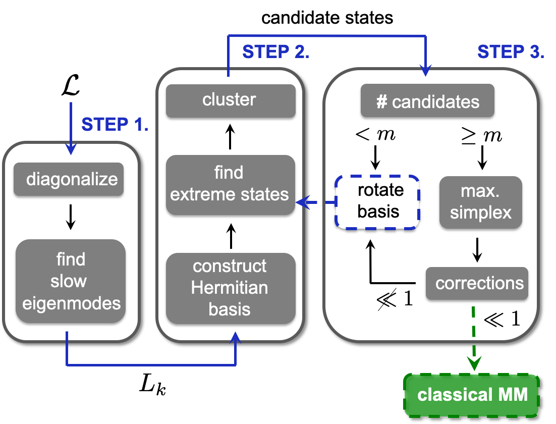
VII.1.1 Metastable phases construction
Our approach consists of the following steps (see also Fig. 6):
- 1.
Diagonalize to find the left eigenmatrices below the gap in the spectrum, .
- 2.
Construct candidate metastable states:
- -
diagonalize the (rotated) eigenmatrices ,
- -
choose the eigenstates associated to their extreme eigenvalues as initial states for candidate metastable states,
- -
discard repetitions in candidate metastable states—cluster in the coefficients space.
- -
- 3.
Find best candidate metastable states:
- i.
- ii.
If the number of candidate states , or the corrections to the classicality in Step 3i are not negligible, then enlarge the set of candidates obtained from Step 3 by considering a random rotation of the basis of the left eigenmatrices in Step 2.
Step 1 in the above construction provides the low-dimensional description of the MM, and, as explained in Sec. III, allows for testing the approximation of the MM as mixtures of candidate states. We choose Hermitian replacing conjugate pairs of eigenmodes , Note2 by
| (83) |
where is an arbitrary phase. Step 2 relies on the result in Sec. 1 of the SM, that metastable states arising from extreme eigenstates of the dynamics eigenmodes can be used to approximate metastable phases in classical MMs, as long as only a single metastable phase is close to the extreme value of the corresponding coefficient (which we refer to as the case without degeneracy); cf. Figs. 2 and 5(a). We then discard any repetitions in the set of candidate states (to treat all coefficients on equal footing, we set the normalization , where and are extreme eigenvalues of ). Indeed, for a given left basis we obtain candidate metastable states corresponding to extreme eigenvalues of the basis elements, which may provide up to metastable phases. In the case without degeneracy, each candidate corresponds to one of metastable phases. In the case with degeneracy, some of extreme eigenstates may correspond to mixtures of metastable phases: provided that the set of candidate states features all metastable phases, such a candidate state should be discarded in Step 3i (this relies on the result from Sec. 3 in the SM, that the simplex of metastable phase is approximately the largest simplex inside the MM; cf. Fig. 2). However, such mixtures may cause less than candidates to remain after clustering, or result in a set of phases which provides a poor approximation to the true MM; even without degeneracy, it is possible that some metastable phases may reside on the interior of the hypercube defined by the extreme values of the coefficients, and as such will not appear in the set of candidate states taken from extreme eigenvalues of the eigenmodes. Nevertheless, random rotations in Step 3ii ensure that each metastable phase is eventually exposed, i.e., a basis in which that metastable phase achieves an extreme coefficient value without degeneracy is eventually considered (with the probability achieved exponentially in the number of rotations; cf. Sec. 2 in the SM). When the set of metastable phases leading to small corrections to the classicality is found, the dual basis in Eq. (20) can be constructed, and the long-time dynamics decomposed as in Eq. (34).
Naturally, instead of considering distances between candidate states in the space of coefficients, as used in Steps 2 and 3i, candidate states can be clustered with respect to the trace distance in the space of density matrices, while the best candidate states can be chosen to achieve minimal corrections to the classicality instead of the maximal simplex volume. These modifications, however, require working with operators on the system Hilbert space, rather than on the space of coefficients, and thus are in general more expensive numerically [for classical MMs, ], while not necessary for MMs with nonnegligible volumes (cf. Secs. 2 and 3 in the SM).
Our approach will not deliver a set of metastable phases with negligible corrections to the classicality whenever the MM is not classical. In particular, quantum MMs Macieszczak et al. 2016a featuring decoherence free subspaces Zanardi 1997; Zanardi and Rasetti 1997; Lidar et al. 1998 or noiseless subsystems Zanardi 2000; Knill et al. 2000: which, e.g., at amount to Bloch-sphere in the coefficient space, rather than a tetrahedron (see also Ref. Bengtsson and Życzkowski 2006), cannot be approximated as probabilistic mixtures of metastable phases. Even for classical metastability emerging in many-body open quantum systems, the approach relies on the condition in Eq. (25), which may be fulfilled only at larger system sizes, when the low-lying part of the master operator spectrum to be sufficiently separated from the fast modes. In this case, our approach may not succeed for smaller system sizes with less pronounced metastability.
While degeneracies are unlikely to occur in a generic model, they typically appear in the presence a hierarchy of metastabilities or as a consequence of symmetries of the dynamics, which we discuss in detail below. In particular, in the presence of a weak symmetry, not only the degeneracy can be efficiently remedied, but also the search for candidates states made even more efficient.
VII.1.2 Construction for hierarchy of metastable manifolds
In the presence of hierarchy of metastabilities with a further separation at in the spectrum of the master operator, the degeneracy appears as a consequence of the fact that the simplex of metastable phases of the first MM, when projected onto the coefficients , is approximated by a simplex with vertices corresponding to metastable phases of the second MM. This requires (at least) metastable phases in the first MM to evolve directly into metastable phases of the second MM. Each of other metastable phases of the first MM either evolves into a single phase of the second MM, or it belongs to the decay subspace in which case it in general evolves into a mixture of metastable phases of the second MM. In the former case, the metastable phases in the first MM that evolve into the same phase in the second MM are degenerate in the coefficients . In the latter case, they do cannot take extreme values of those coefficients, even after a rotation of the first modes (see Secs. 1 and 4 in the SM). Nevertheless, rotations of all modes allow both for the degeneracy to be lifted and for every metastable phase to take an extreme value in one of the coefficients.
VII.1.3 Construction for metastable manifolds with symmetries
In the presence of a weak symmetry [Eq. (67)], the master operator is block diagonal in the eigenspaces of , which simplifies its diagonalization Baumgartner and Narnhofer 2008; Buča and Prosen 2012; Albert and Jiang 2014. As a consequence, the low-lying eigenmodes of the dynamics are chosen as linear combinations of the plane waves over the cycles induced by the symmetry on metastable phases [cf. Eq. (81)]. In particular, for an eigenmode , with a symmetry eigenvalue , , and the minimal integer leading to , is supported on cycles with the length equal or larger but divisible by . The latter case, of subcycles with length , leads to degeneracy of the coefficient for the metastable phases connected by , with its extreme eigenstates generically projecting onto their uniform mixture [cf. Eq. (80b) and Fig. 5(a), where and are degenerate in and ()]. Nevertheless, coefficient degeneracy can be remedied and the structure of the low-lying eigenmodes can be used to actually enhance the introduced approach, as we now explain (see also Sec. 5 in the SM).
We note that when for all , , the eigenmode is supported only on cycles of length , as there are no longer cycles with the length divisible by . The symmetry then acts trivially on the corresponding metastable phases and the above discussed degeneracy is absent. Analogously to the general case, any plane wave in can then be exposed by random rotations of the eigenmodes with the same symmetry eigenvalue , while at least a single metastable phase from each cycle can be obtained by considering extreme eigenstates of both and 1616 16 For not divisible by , otherwise see Sec. c in the SM.. Other metastable phases in the considered cycles can be recovered by applying the symmetry times, so there is no need to consider eigenmodes with a different symmetry eigenvalue supported on the same cycles (i.e., with but ).
Furthermore, metastable phases in cycles with the length corresponding to subcycles, e.g., invariant metastable phases, can also be found. For such that is divides only for the above considered eigenmodes , when the degeneracy of equals the number of already considered cycles with divisible by (i.e., the sum of the corresponding symmetry eigenvalue degeneracy for all such values), is supported on the already considered cycles. Otherwise, features new cycles with the length , which can be unfolded, as before, by rotations of all eigenmodes with the same symmetry eigenvalue as and considering both and Note16. Here, equal mixtures of already considered phases connected by will also be found, but such candidate states will not lead to the maximal volume simplex. Again, by applying symmetry the full (sub)cycles can be recovered, and other eigenmodes with , but a different symmetry eigenvalue can be discarded. Analogous results hold for the remaining eigenmodes, but with respect to and degeneracy.
In summary, the set of eigenmodes considered in Step 2 is significantly reduced, with its size equal to the number of cycles and the subcycles with other cycle’s length. Furthermore, only rotations of eigenmodes with the same symmetry eigenvalue are necessary in Step 3ii. Importantly, as the eigenstates of and and the corresponding metastable states are invariant under , that is, generate cycles of candidate states with the length dividing , following the prescription above, we arrive at an invariant set of candidate states. This invariance can be maintained by clustering whole cycles of candidate states rather than individual states in Step 2. Then, without loss of generality, in Step 3i, instead of considering subsets of all candidate states, we can choose candidate states as sets of cycles with their lengths summing to . In that case, the volume of the simplex can be efficiently calculated as , where is the block-diagonal matrix in Eq. (82) and the product, which runs over cycle representatives, is the same for all sets of linearly independent candidates Note14, while the corrections to the classicality can be efficiently calculated with the symmetric test of classicality of Sec. VI.2.5.
VII.1.4 Construction utilizing order parameters
Instead of considering the eigenmodes of the dynamics, we can choose a left eigenbasis formed by a set of observables , projected onto the low-lying eigenmodes, i.e., , where [cf. Eq. (4)], provided that those projections are linearly independent. In this case, the extreme eigenstates of will give metastable states attaining extreme values in the average of the observable . Those metastable states will correspond to metastable phases, up to degeneracy of metastable phase averages of (in particular, in the presence of nontrivial weak symmetry of low-lying eigenmodes, it is necessary to consider observables breaking the symmetry). Among others, this can be helpful when the volume of MM in the space of coefficients is negligible. In the next section, we extend this approach by considering continuous measurements instead of system observables.
VII.2 Metastable phases from biased quantum trajectories
In some systems, the metastability can be a collective effect emerging as the system size increases Rose et al. 2016. If large system sizes are required for prominent metastability, then exact diagonalization may not be feasible. Therefore, we now introduce an alternative numerical approach to finding metastable phases in classical MMs using QJMC simulations Dalibard et al. 1992; Dum et al. 1992; Mølmer et al. 1993; Plenio and Knight 1998; Daley 2014 and biased sampling in the framework of large deviation theory (see Ref. Touchette 2009 for a review). In classical stochastic dynamics biased sampling can be efficiently incorporated into the generation of trajectories, with techniques such as transition path sampling Hedges et al. 2009 and cloning Giardina et al. 2011.
Trajectories of the biased master equation in Eq. (44) can be viewed as trajectories of with their probability multiplied by , where is the total number of jumps occurring in a quantum trajectory of length . The maximal eigenmode of corresponds then to the asymptotic system state in quantum trajectories averaged with the biased probability. In Sec. V.2.5, we argued that can approximate metastable phases of extreme activity for appropriately chosen when the activity dominates the transition rates of long-time dynamics [cf. Figs. 4(a) and 4(c)]. Thus, if the efficient biased sampling could be generalized to QJMC sampling, metastable phases with extreme activity could be accessed via time-average of a biased trajectory over time-length within the metastable regime 1717 17 The timescale of the relaxation toward in the biased dynamics belongs to the metastable regime when Eqs. (63) and (64) hold. Indeed, due to the separation also present in the spectrum of is approximated by the relaxation time of of Eq. (62) and negligible corrections from fast modes of give . Moreover, as can be neglected in Eq. (62)], ..
Similarly as in the case of degeneracy of coefficients, when more than a single metastable phase corresponds to the maximum or the minimum activity, corresponds to a mixture of the metastable phases with the extreme value (e.g., when both and obey a symmetry that is broken in the MM, the mixture is symmetric). Nevertheless, the discussion in Sec. V.2.5 is analogous for the activity of individual jumps, and thus a further distinction between metastable phases can be enabled this way, e.g., by breaking the translation symmetry of in the case of identical local jumps (see Sec. a in the SM). Finally, we note that in the case of general metastability, this approach will return the metastable states corresponding to the extreme values of jump activity.
VIII Conclusions and outlook
In this paper, we formulated a comprehensive theory for the emergence of classical metastability for open quantum systems whose dynamics is governed by a master operator. We showed that classical metastability is characterized by the approximation of metastable states as probabilistic mixtures of metastable phases, where is the number of low-lying modes of the master operator. Namely, in terms of the corresponding corrections, metastable phases are approximately disjoint, while the long-time dynamics, both on average and in individual quantum trajectories, is approximately governed by an effective classical stochastic generator. Furthermore, any nontrivial weak symmetries present at long times are necessarily discrete as they correspond to approximate permutations of metastable phases, under which the classical dynamics is invariant. To investigate metastability for a given open quantum system, we introduced the test of classicality—an approach to verify the approximation of the MM by a set of candidate metastable phases. We also developed a complementary numerical approach to deliver sets of candidate metastable phases. Since that approach requires diagonalization of the master operator—a difficult task in systems of larger size—we also discussed an alternative based on the concept of biased trajectory sampling.
The techniques we introduced here allow us to achieve a complete understanding of classical metastability emerging in an open quantum system. A concrete application of the methods described here to a many-body system of an open quantum East model Olmos et al. 2012 is given in Ref. Rose et al. 2020, where despite the stationary state being analytic in dynamics parameters, the dynamics is found to feature a hierarchy of classical metastabilities, with metastable phases breaking the translation symmetry of the model and their number increasing with the system size. This structure is then shown to be analogous to metastability in the classical East model, but with an effective temperature and coherent excitations.
While our general approach relies only on the Markovian approximation of system dynamics, non-Markovian effects could be includedvia the chain partial diagonalization Burkey and Cantrell 1984; Chin et al. 2010; Woods et al. 2014 (see also Ref. Iles-Smith et al. 2014). However, an open quantum system and its environment form an isolated system, which raises a question about the relation of classical metastability to separation of timescales in closed system dynamics, which generically leads to prethermalization of subsystem states Gring et al. 2012. Furthermore, as in this work no assumptions were made on the structure of system Hamiltonian or jump operators, it should be explored how metastable phases and their basins of attraction can be further characterized in systems with local interactions and local dissipation (see also Ref. Landa et al. 2020). Finally, it remains an open question what is the structure of general quantum metastability and how it can be efficiently investigated, e.g., to uncover metastable coherences Macieszczak et al. 2016a. Extending the methods described here to this general case would inform, among others, the study of a general structure of first-order dissipative phase transitions in open quantum systems.
Acknowledgements.
K.M. thanks M. Guţă for helpful discussions. K.M. gratefully acknowledges support from a Henslow Research Fellowship. We acknowledge financial support from EPSRC Grant No. EP/R04421X/1, from the H2020-FETPROACT-2014 Grant No. 640378 (RYSQ), and by University of Nottingham Grant No. FiF1/3. I.L. acknowledges support by the “Wissenschaftler-Rückkehrprogramm GSO/CZS” of the Carl-Zeiss-Stiftung, through the Deutsche Forschungsgemeinsschaft (DFG, German Research Foundation) under Project No. 435696605 and through the European Union’s H2020 research and innovation programme [Grant Agreement No. 800942 (ErBeStA)]. We are grateful for access to the University of Nottingham Augusta HPC service.References
- Pritchard et al. (2010) J. D. Pritchard, D. Maxwell, A. Gauguet, K. J. Weatherill, M. P. A. Jones, and C. S. Adams, “Cooperative Atom-Light Interaction in a Blockaded Rydberg Ensemble,” Phys. Rev. Lett. 105, 193603 (2010).
- Blatt and Roos (2012) R. Blatt and C. F. Roos, “Quantum simulations with trapped ions,” Nat. Phys. 8, 277–284 (2012).
- Britton et al. (2012) J. W. Britton, B. C. Sawyer, A. C. Keith, C. C. J. Wang, J. K. Freericks, H. Uys, M. J. Biercuk, and J. J. Bollinger, “Engineered two-dimensional Ising interactions in a trapped-ion quantum simulator with hundreds of spins,” Nature 484, 489–492 (2012).
- Dudin and Kuzmich (2012) Y. O. Dudin and A. Kuzmich, “Strongly Interacting Rydberg Excitations of a Cold Atomic Gas,” Science 336, 887–889 (2012).
- Peyronel et al. (2012) T. Peyronel, O. Firstenberg, Q. Liang, S. Hofferberth, A. V. Gorshkov, T. Pohl, M. D. Lukin, and V. Vuletic, “Quantum nonlinear optics with single photons enabled by strongly interacting atoms,” Nature 488, 57–60 (2012).
- Günter et al. (2013) G. Günter, H. Schempp, M. Robert-de Saint-Vincent, V. Gavryusev, S. Helmrich, C. S. Hofmann, S. Whitlock, and M. Weidemüller, “Observing the Dynamics of Dipole-Mediated Energy Transport by Interaction-Enhanced Imaging,” Science 342, 954–956 (2013).
- Schmidt and Koch (2013) S. Schmidt and J. Koch, “Circuit QED lattices: Towards quantum simulation with superconducting circuits,” Ann. Phys. 525, 395–412 (2013).
- Dalibard et al. (1992) J. Dalibard, Y. Castin, and K. Mølmer, “Wave-function approach to dissipative processes in quantum optics,” Phys. Rev. Lett. 68, 580–583 (1992).
- Dum et al. (1992) R. Dum, A. S. Parkins, P. Zoller, and C. W. Gardiner, “Monte Carlo simulation of master equations in quantum optics for vacuum, thermal, and squeezed reservoirs,” Phys. Rev. A 46, 4382–4396 (1992).
- Mølmer et al. (1993) K. Mølmer, Y. Castin, and J. Dalibard, “Monte Carlo wave-function method in quantum optics,” J. Opt. Soc. Am. B 10, 524–538 (1993).
- Plenio and Knight (1998) M. B. Plenio and P. L. Knight, “The quantum-jump approach to dissipative dynamics in quantum optics,” Rev. Mod. Phys. 70, 101–144 (1998).
- Daley (2014) A. J. Daley, “Quantum trajectories and open many-body quantum systems,” Adv. Phys. 63, 77–149 (2014).
- Gangat et al. (2017) A. A. Gangat, T. I, and Y.-J. Kao, “Steady States of Infinite-Size Dissipative Quantum Chains via Imaginary Time Evolution,” Phys. Rev. Lett. 119, 010501 (2017).
- Torre et al. (2013) E. G. D. Torre, S. Diehl, M. D. Lukin, S. Sachdev, and P. Strack, “Keldysh approach for nonequilibrium phase transitions in quantum optics: Beyond the Dicke model in optical cavities,” Phys. Rev. A 87, 023831 (2013).
- Sieberer et al. (2016) L. M. Sieberer, M. Buchhold, and S. Diehl, “Keldysh field theory for driven open quantum systems,” Rep. Prog. Phys. 79, 096001 (2016).
- Maghrebi and Gorshkov (2016) M. F. Maghrebi and A. V. Gorshkov, “Nonequilibrium many-body steady states via Keldysh formalism,” Phys. Rev. B 93, 014307 (2016).
- Mendoza-Arenas et al. (2016) J. J. Mendoza-Arenas, S. R. Clark, S. Felicetti, G. Romero, E. Solano, D. G. Angelakis, and D. Jaksch, “Beyond mean-field bistability in driven-dissipative lattices: Bunching-antibunching transition and quantum simulation,” Phys. Rev. A 93, 023821 (2016).
- Foss-Feig et al. (2017) M. Foss-Feig, P. Niroula, J. T. Young, M. Hafezi, A. V. Gorshkov, R. M. Wilson, and M. F. Maghrebi, “Emergent equilibrium in many-body optical bistability,” Phys. Rev. A 95, 043826 (2017).
- Casteels and Wouters (2017) W. Casteels and M. Wouters, “Optically bistable driven-dissipative Bose-Hubbard dimer: Gutzwiller approaches and entanglement,” Phys. Rev. A 95, 043833 (2017).
- Letscher et al. (2017) F. Letscher, O. Thomas, T. Niederprüm, M. Fleischhauer, and H. Ott, “Bistability Versus Metastability in Driven Dissipative Rydberg Gases,” Phys. Rev. X 7, 021020 (2017).
- Jin et al. (2018) J. Jin, A. Biella, O. Viyuela, C. Ciuti, R. Fazio, and D. Rossini, “Phase diagram of the dissipative quantum Ising model on a square lattice,” Phys. Rev. B 98, 241108 (2018).
- de Melo et al. (2016) N. R. de Melo, C. G. Wade, N. Šibalić, J. M. Kondo, C. S. Adams, and K. J. Weatherill, “Intrinsic optical bistability in a strongly driven Rydberg ensemble,” Phys. Rev. A 93, 063863 (2016).
- Rodriguez et al. (2017) S. R. K. Rodriguez, W. Casteels, F. Storme, N. Carlon Zambon, I. Sagnes, L. Le Gratiet, E. Galopin, A. Lemaître, A. Amo, C. Ciuti, and J. Bloch, “Probing a Dissipative Phase Transition via Dynamical Optical Hysteresis,” Phys. Rev. Lett. 118, 247402 (2017).
- Ates et al. (2012) C. Ates, B. Olmos, J. P. Garrahan, and I. Lesanovsky, “Dynamical phases and intermittency of the dissipative quantum Ising model,” Phys. Rev. A 85, 043620 (2012).
- Landa et al. (2020) H. Landa, M. Schiró, and G. Misguich, “Multistability of Driven-Dissipative Quantum Spins,” Phys. Rev. Lett. 124, 043601 (2020).
- Weimer (2015a) H. Weimer, “Variational Principle for Steady States of Dissipative Quantum Many-Body Systems,” Phys. Rev. Lett. 114, 040402 (2015a).
- Weimer (2015b) H. Weimer, “Variational analysis of driven-dissipative Rydberg gases,” Phys. Rev. A 91, 063401 (2015b).
- Overbeck et al. (2017) V. R. Overbeck, M. F. Maghrebi, A. V. Gorshkov, and H. Weimer, “Multicritical behavior in dissipative Ising models,” Phys. Rev. A 95, 042133 (2017).
- Biondi et al. (2017) M. Biondi, S. Lienhard, G. Blatter, H. E. Türeci, and S. Schmidt, “Spatial correlations in driven-dissipative photonic lattices,” New J. Phys. 19, 125016 (2017).
- Spohn (1977) H. Spohn, “An algebraic condition for the approach to equilibrium of an open N-level system,” Lett. Math. Phys. 2, 33–38 (1977).
- Evans (1977) D. E. Evans, “Irreducible quantum dynamical semigroups,” Comm. Math. Phys. 54, 293–297 (1977).
- Schirmer and Wang (2010) S. G. Schirmer and X. Wang, “Stabilizing open quantum systems by Markovian reservoir engineering,” Phys. Rev. A 81, 062306 (2010).
- Nigro (2019) D. Nigro, “On the uniqueness of the steady-state solution of the Lindblad–Gorini–Kossakowski–Sudarshan equation,” J. Stat. Mech. 2019, 043202 (2019).
- Chaikin and Lubensky (2000) P. M. Chaikin and T. C. Lubensky, Principles of condensed matter physics, Vol. 1 (Cambridge University Press, 2000).
- Gaveau and Schulman (1987) B. Gaveau and L. S. Schulman, “Dynamical metastability,” J. Phys. A 20, 2865 (1987).
- Gaveau and Schulman (1998) B. Gaveau and L. S. Schulman, “Theory of nonequilibrium first-order phase transitions for stochastic dynamics,” J. Mat. Phys. 39, 1517 (1998).
- Bovier et al. (2002) A. Bovier, M. Eckhoff, V. Gayrard, and M. Klein, “Metastability and Low Lying Spectra in Reversible Markov Chains,” Comm. Math. Phys 228, 219 (2002).
- Gaveau and Schulman (2006) B. Gaveau and L. S. Schulman, “Multiple phases in stochastic dynamics: Geometry and probabilities,” Phys. Rev. E 73, 036124 (2006).
- Kurchan (2016) J. Kurchan, “Six out of equilibrium lectures,” (2016), arXiv:0901.1271 .
- Macieszczak et al. (2016a) K. Macieszczak, M. Guta, I. Lesanovsky, and J. P. Garrahan, “Towards a Theory of Metastability in Open Quantum Dynamics,” Phys. Rev. Lett. 116, 240404 (2016a).
- Rose et al. (2016) D. C. Rose, K. Macieszczak, I. Lesanovsky, and J. P. Garrahan, “Metastability in an open quantum Ising model,” Phys. Rev. E 94, 052132 (2016).
- Minganti et al. (2018) F. Minganti, A. Biella, N. Bartolo, and C. Ciuti, “Spectral theory of Liouvillians for dissipative phase transitions,” Phys. Rev. A 98, 042118 (2018).
- Jäckle and Eisinger (1991) J. Jäckle and S. Eisinger, “A hierarchically constrained kinetic Ising model,” Z. Phys. B 84, 115–124 (1991).
- Sollich and Evans (1999) P. Sollich and M. R. Evans, “Glassy Time-Scale Divergence and Anomalous Coarsening in a Kinetically Constrained Spin Chain,” Phys. Rev. Lett. 83, 3238–3241 (1999).
- Garrahan and Chandler (2002) J. P. Garrahan and D. Chandler, “Geometrical Explanation and Scaling of Dynamical Heterogeneities in Glass Forming Systems,” Phys. Rev. Lett. 89, 035704 (2002).
- Sollich and Evans (2003) P. Sollich and M. R. Evans, “Glassy dynamics in the asymmetrically constrained kinetic Ising chain,” Phys. Rev. E 68, 031504 (2003).
- Binder and Kob (2011) K. Binder and W. Kob, Glassy Materials and Disordered Solids: An Introduction to Their Statistical Mechanics (Revised Edition) (World Scientific, 2011).
- Biroli and Garrahan (2013) G. Biroli and J. P. Garrahan, “Perspective: The glass transition,” J. Chem. Phys. 138, 12A301 (2013).
- Binder and Young (1986) K. Binder and A. P. Young, “Spin glasses: Experimental facts, theoretical concepts, and open questions,” Rev. Mod. Phys. 58, 801–976 (1986).
- Olmos et al. (2012) B. Olmos, I. Lesanovsky, and J. P. Garrahan, “Facilitated Spin Models of Dissipative Quantum Glasses,” Phys. Rev. Lett. 109, 020403 (2012).
- Lesanovsky et al. (2013) I. Lesanovsky, M. van Horssen, M. Guţă, and J. P. Garrahan, “Characterization of Dynamical Phase Transitions in Quantum Jump Trajectories Beyond the Properties of the Stationary State,” Phys. Rev. Lett. 110, 150401 (2013).
- Olmos et al. (2014) B. Olmos, I. Lesanovsky, and J. P. Garrahan, “Out-of-equilibrium evolution of kinetically constrained many-body quantum systems under purely dissipative dynamics,” Phys. Rev. E 90, 042147 (2014).
- Cugliandolo and Lozano (1999) L. F. Cugliandolo and G. Lozano, “Real-time nonequilibrium dynamics of quantum glassy systems,” Phys. Rev. B 59, 915–942 (1999).
- Rose et al. (2020) D. C. Rose, K. Macieszczak, I. Lesanovsky, and J. P. Garrahan, “Hierarchical classical metastability in an open quantum East model,” (2020), arXiv:2010.15304 .
- Thingna et al. (2016) J. Thingna, D. Manzano, and J. Cao, “Dynamical signatures of molecular symmetries in nonequilibrium quantum transport,” Sci. Rep. 6, 28027 (2016).
- Lindblad (1976) G. Lindblad, “On the generators of quantum dynamical semigroups,” Commun. Math. Phys. 48, 119–130 (1976).
- Gorini et al. (1976) V. Gorini, A. Kossakowski, and E. C. G. Sudarshan, “Completely positive dynamical semigroups of N-level systems,” J. Math. Phys. 17, 821–825 (1976).
- Gardiner and Zoller (2004) C. W. Gardiner and P. Zoller, Quantum Noise, 3rd ed., Complexity (Springer, 2004).
- Garrahan and Lesanovsky (2010) J. P. Garrahan and I. Lesanovsky, “Thermodynamics of Quantum Jump Trajectories,” Phys. Rev. Lett. 104, 160601 (2010).
- Baumgartner and Narnhofer (2008) B. Baumgartner and H. Narnhofer, “Analysis of quantum semigroups with GKS–Lindblad generators: II. General,” J. Phys. A 41, 395303 (2008).
- Buča and Prosen (2012) B. Buča and T. Prosen, “A note on symmetry reductions of the Lindblad equation: transport in constrained open spin chains,” New J. Phys. 14, 073007 (2012).
- Albert and Jiang (2014) V. V. Albert and L. Jiang, “Symmetries and conserved quantities in Lindblad master equations,” Phys. Rev. A 89, 022118 (2014).
- Garrahan et al. (2011) J. P. Garrahan, A. D. Armour, and I. Lesanovsky, “Quantum trajectory phase transitions in the micromaser,” Phys. Rev. E 84, 021115 (2011).
- Carollo et al. (2018) F. Carollo, J. P. Garrahan, I. Lesanovsky, and C. Pérez-Espigares, “Making rare events typical in Markovian open quantum systems,” Phys. Rev. A 98, 010103 (2018).
- (65) It is possible that the master operator may not be completely diagonalizable, in which this case its simplest form is the Jordan normal form. Under exponentiation, this gives rise to a polynomial dependence on the time, however this is accompanied by the usual exponential evolution. Our results in Secs. III, IV, V.1, VI, and VII carry directly to that case by assuming that after the initial relaxation, any polynomial evolution of fast modes is dominated by the decaying exponential and can be neglected [cf. Eq. (3)], while during the metastable regime dynamics of the slow modes can be replaced by no evolution [cf. Eq. (4)]. In Sec. V.2, the corrections to Eqs. (54) and (61) need to be adjusted, together with corresponding Secs. e, f, and h in the SM.
- Albert et al. (2016) V. V. Albert, B. Bradlyn, M. Fraas, and L. Jiang, “Geometry and Response of Lindbladians,” Phys. Rev. X 6, 041031 (2016).
- Bellomo et al. (2017) B. Bellomo, G. L. Giorgi, G. M. Palma, and R. Zambrini, “Quantum synchronization as a local signature of super- and subradiance,” Phys. Rev. A 95, 043807 (2017).
- (68) Since is Hermiticity preserving, if () is a right (left) eigenmode of the dynamics with an eigenvalue , so is () with the eigenvalue . Thus the set of low-lying modes is invariant under the Hermitian conjugation.
- Sciolla et al. (2015) B. Sciolla, D. Poletti, and C. Kollath, “Two-Time Correlations Probing the Dynamics of Dissipative Many-Body Quantum Systems: Aging and Fast Relaxation,” Phys. Rev. Lett. 114, 170401 (2015).
- (70) We restrict the discussion to the real space of Hermitian operators. In this case, the induced norm of a superoperator can be shown to be achieved for a pure state (i.e., a rank one operator). Let be a Hermitian operator with eigenvalues and projections on the corresponding eigenstates denoted as . For a superoperator , we have .
- (71) For an integer such that , we have . Since we have [cf. Eq. (10)], while [cf. Eq. (12)], we arrive at .
- (72) For an integer such that , we have , where due to , while .
- Zanardi (1997) P. Zanardi, “Dissipative dynamics in a quantum register,” Phys. Rev. A 56, 4445–4451 (1997).
- Zanardi and Rasetti (1997) P. Zanardi and M. Rasetti, “Noiseless Quantum Codes,” Phys. Rev. Lett. 79, 3306–3309 (1997).
- Lidar et al. (1998) D. A. Lidar, I. L. Chuang, and K. B. Whaley, “Decoherence-Free Subspaces for Quantum Computation,” Phys. Rev. Lett. 81, 2594–2597 (1998).
- Knill et al. (2000) E. Knill, R. Laflamme, and L. Viola, “Theory of Quantum Error Correction for General Noise,” Phys. Rev. Lett. 84, 2525–2528 (2000).
- Zanardi (2000) P. Zanardi, “Stabilizing quantum information,” Phys. Rev. A 63, 012301 (2000).
- Zanardi and Campos Venuti (2014) P. Zanardi and L. Campos Venuti, “Coherent Quantum Dynamics in Steady-State Manifolds of Strongly Dissipative Systems,” Phys. Rev. Lett. 113, 240406 (2014).
- Zanardi and Campos Venuti (2015) P. Zanardi and L. Campos Venuti, “Geometry, robustness, and emerging unitarity in dissipation-projected dynamics,” Phys. Rev. A 91, 052324 (2015).
- Zanardi et al. (2016) P. Zanardi, J. Marshall, and L. Campos Venuti, “Dissipative universal Lindbladian simulation,” Phys. Rev. A 93, 022312 (2016).
- Popkov et al. (2018) V. Popkov, S. Essink, C. Presilla, and G. Schütz, “Effective quantum zeno dynamics in dissipative quantum systems,” Phys. Rev. A 98, 052110 (2018).
- (82) We have , where we used the left-eigenmatrix normalization with and denoting the maximal and minimal eigenvalue of . We then choose time within the metastable regime for which is minimal.
- (83) We have , where , , encodes the coefficients for the simplex with the vertex of shifted to the origin.
- Życzkowski and Sommers (2001) K. Życzkowski and H.-J. Sommers, “Induced measures in the space of mixed quantum states,” J. Phys. A 34, 7111 (2001).
- Życzkowski and Sommers (2003) K. Życzkowski and H.-J. Sommers, “Hilbert–Schmidt volume of the set of mixed quantum states,” J. Phys. A 36, 10115 (2003).
- (86) We note that often the diamond norm, , is used instead of induced trace norm, , to quantify the disturbance caused by a quantum channel with respect to the identity channel .
- Wolf (2012) M. M. Wolf, Quantum channels and Operations, Guided tour (2012).
- Nielsen and Chuang (2010) M. A. Nielsen and I. L. Chuang, Quantum Computation and Quantum Information (Cambridge University Press, 10th Anniversary ed. edition, 2010).
- Gaveau et al. (1999) B. Gaveau, A. Lesne, and L. S. Schulman, “Spectral signatures of hierarchical relaxation,” Phys. Lett. A 258, 222 – 228 (1999).
- (90) is the matrix norm induced by the L1 norm of vectors. For a vector and a matrix , we have , and the inequality can be saturated by considering basis vectors.
- (91) We note that an analogous approximation of the stationary state can be also obtained by considering non-Hermitian perturbation theory for with respect to perturbation of (see Sec. d in the SM).
- (92) Due to the exponential decay of and , this will be typically implied by Eq. (40); cf. Sec. 3 c in the SM.
- Smirne et al. (2018) A. Smirne, D. Egloff, M. G. Díaz, M. B. Plenio, and S. F. Huelga, “Coherence and non-classicality of quantum Markov processes,” Quantum Science and Technology 4, 01LT01 (2018).
- Kato (1995) T. Kato, Perturbation Theory for Linear Operators (Springer, 1995).
- Levitov et al. (1996) L. S. Levitov, H. Lee, and G. B. Lesovik, “Electron counting statistics and coherent states of electric current,” J. Math. Phys. 37, 4845–4866 (1996).
- Nazarov and Division (2003) Y. V. Nazarov and N. A. T. O. S. A. Division, Quantum Noise in Mesoscopic Physics, NATO Science Series: Mathematics, Physics and Chemistry (Springer, New York, 2003).
- Esposito et al. (2009) M. Esposito, U. Harbola, and S. Mukamel, “Nonequilibrium fluctuations, fluctuation theorems, and counting statistics in quantum systems,” Rev. Mod. Phys. 81, 1665–1702 (2009).
- Flindt et al. (2009) C. Flindt, C. Fricke, F. Hohls, T. Novotný, K. Netočný, T. Brandes, and R. J. Haug, “Universal oscillations in counting statistics,” Proc. Natl. Acad. Sci. 106, 10116–10119 (2009).
- Hickey et al. (2012) J. M. Hickey, S. Genway, I. Lesanovsky, and J. P. Garrahan, “Thermodynamics of quadrature trajectories in open quantum systems,” Phys. Rev. A 86, 063824 (2012).
- Hickey et al. (2013) J. M. Hickey, S. Genway, I. Lesanovsky, and J. P. Garrahan, “Time-integrated observables as order parameters for full counting statistics transitions in closed quantum systems,” Phys. Rev. B 87, 184303 (2013).
- Lecomte et al. (2007) V. Lecomte, C. Appert-Rolland, and F. van Wijland, “Thermodynamic formalism for systems with Markov dynamics,” J. Stat. Phys. 127, 51 (2007).
- Garrahan et al. (2007) J. P. Garrahan, R. L. Jack, V. Lecomte, E. Pitard, K. van Duijvendijk, and F. van Wijland, “Dynamical First-Order Phase Transition in Kinetically Constrained Models of Glasses,” Phys. Rev. Lett. 98, 195702 (2007).
- Maes (2020) C. Maes, “Frenesy: Time-symmetric dynamical activity in nonequilibria,” Phys. Rep. 850, 1 – 33 (2020).
- Garrahan (2018) J. P. Garrahan, “Aspects of non-equilibrium in classical and quantum systems: Slow relaxation and glasses, dynamical large deviations, quantum non-ergodicity, and open quantum dynamics,” Physica A 504, 130–154 (2018).
- Jack (2020) R. L. Jack, “Ergodicity and large deviations in physical systems with stochastic dynamics,” Eur. Phys. J. B 93, 74 (2020).
- (106) can be further replaced by , with being a real constant and the norm minimized with respect to in the corrections; see Sec. d in the SM.
- Gammelmark and Mølmer (2014) S. Gammelmark and K. Mølmer, “Fisher Information and the Quantum Cramér-Rao Sensitivity Limit of Continuous Measurements,” Phys. Rev. Lett. 112, 170401 (2014).
- Macieszczak et al. (2016b) K. Macieszczak, M. Guţă, I. Lesanovsky, and J. P. Garrahan, “Dynamical phase transitions as a resource for quantum enhanced metrology,” Phys. Rev. A 93, 022103 (2016b).
- (109) In Eq. (71) we require for all prime factors of (see Sec. a in the SM).
- Gough et al. (2015) J. E. Gough, T. S. Ratiu, and O. G. Smolyanov, “Noether’s theorem for dissipative quantum dynamical semi-groups,” J. Math. Phys. 56, 022108 (2015).
- (111) When momenta of plane waves over candidate state cycles do not correspond to arguments of symmetry eigenvalues for the low-lying eigenmodes, is not invertible and .
- (112) This follows from the spectrum of any operator unchanged under the action of the symmetry, and . Alternatively, the minimal eigenvalue can be found from the wave-plane basis by considering averages of maximized over , which can be restricted to symmetric states [cf. Eq. (80b)].
- Blume-Kohout et al. (2008) R. Blume-Kohout, H. K. Ng, D. Poulin, and L. Viola, “Characterizing the Structure of Preserved Information in Quantum Processes,” Phys. Rev. Lett. 100, 030501 (2008).
- Blume-Kohout et al. (2010) R. Blume-Kohout, H. K. Ng, D. Poulin, and L. Viola, “Information-preserving structures: A general framework for quantum zero-error information,” Phys. Rev. A 82, 062306 (2010).
- Holbrook et al. (2004) J. A. Holbrook, D. W. Kribs, and R. Laflamme, “Noiseless subsystems and the structure of the commutant in quantum error correction,” Quant. Inf. Proc. 2, 381–419 (2004).
- Choi and Kribs (2006) M.-D. Choi and D. W. Kribs, “Method to Find Quantum Noiseless Subsystems,” Phys. Rev. Lett. 96, 050501 (2006).
- Żurek (1993) W. H. Żurek, “Preferred States, Predictability, Classicality and the Environment-Induced Decoherence,” Progress of Theoretical Physics 89, 281–312 (1993).
- Bengtsson and Życzkowski (2006) C. I. Bengtsson and K. Życzkowski, Geometry of Quantum States: An Introduction to Quantum Entanglement (Cambridge University Press, 2006).
- (119) For not divisible by , otherwise see Sec. c in the SM.
- Touchette (2009) H. Touchette, “The large deviation approach to statistical mechanics,” Phys. Rep. 478, 1 – 69 (2009).
- Hedges et al. (2009) L. O. Hedges, R. L. Jack, J. P. Garrahan, and D. Chandler, “Dynamic Order-Disorder in Atomistic Models of Structural Glass Formers,” Science 323, 1309–1313 (2009).
- Giardina et al. (2011) C. Giardina, J. Kurchan, V. Lecomte, and J. Tailleur, “Simulating Rare Events in Dynamical Processes,” J. Stat. Phys. 145, 787–811 (2011).
- (123) The timescale of the relaxation toward in the biased dynamics belongs to the metastable regime when Eqs. (63) and (64) hold. Indeed, due to the separation also present in the spectrum of is approximated by the relaxation time of of Eq. (62) and negligible corrections from fast modes of give . Moreover, as can be neglected in Eq. (62)], .
- Burkey and Cantrell (1984) R. S. Burkey and C. D. Cantrell, “Discretization in the quasi-continuum,” J. Opt. Soc. Am. B 1, 169–175 (1984).
- Chin et al. (2010) A. W. Chin, A. Rivas, S. F. Huelga, and M. B. Plenio, “Exact mapping between system-reservoir quantum models and semi-infinite discrete chains using orthogonal polynomials,” J. Math. Phys. 51, 092109 (2010).
- Woods et al. (2014) M. P. Woods, R. Groux, A. W. Chin, S. F. Huelga, and M. B. Plenio, “Mappings of open quantum systems onto chain representations and Markovian embeddings,” J. Math. Phys. 55, 032101 (2014).
- Iles-Smith et al. (2014) J. Iles-Smith, N. Lambert, and A. Nazir, “Environmental dynamics, correlations, and the emergence of noncanonical equilibrium states in open quantum systems,” Phys. Rev. A 90, 032114 (2014).
- Gring et al. (2012) M. Gring, M. Kuhnert, T. Langen, T. Kitagawa, B. Rauer, M. Schreitl, I. Mazets, D. A. Smith, E. Demler, and J. Schmiedmayer, “Relaxation and Prethermalization in an Isolated Quantum System,” Science 337, 1318–1322 (2012).
Theory of classical metastability in open quantum systems
Supplemental Material
In this Supplemental Material, we provide proofs of the results in "Theory of classical metastability in open quantum systems". The open quantum system which serves as the illustration of our general results in Figs. 1–5 of the main text is discussed in Sec. A, together with classical metastability arising in proximity to dissipative phase transitions at finite size. The derivations for the quantitative approach to metastability are given in Sec. B. Then proofs are given of the following results: classical metastability in Sec. C, classical metastable phases in Sec. D, classical long-time dynamics in Sec. E, classical hierarchy of metastabilities in Sec. F, and classical weak symmetries in Sec. G. Finally, the correctness of the new numerical approach introduced in the main text is argued in Sec. H.
A Classical metastability in proximity to dissipative phase transition at finite size
Here, we first describe the model we illustrate our general theory of metastability in Markovian open quantum systems with in Figs. 1–5 of the main text. This example belongs to a class of systems where classical metastability is a consequence of perturbing dynamical parameters away from effectively classical dissipative phase transitions occurring at a finite size. Second, we find and discuss the general structure of metastable phases and long-time dynamics for this class.
1 Example in Figs. 1–5 of the main text
a Model
In Figs. 1–4 of the main text, we choose a system of levels , , connected in the Markovian dynamics governed by the master operator in Eq. (1), with the Hamiltonian
| (A1) |
where , and the dissipative jumps
| (A2) | |||||
| (A3) |
where , as depicted in Fig. A1. We assume and correspond to emission of quanta [cf. Fig. 1(e) in the main text].
In Fig. 5 of the main text, we replace in Eq. (A3) by . This introduces a discrete weak symmetry under the simultaneous swap and (cf. Fig. A1 and see Sec. VI in the main text).

b Dissipative phase transition
In the limit
| (A4) |
the dynamics is in the proximity of a dissipative phase transition with four independent sectors corresponding to: two decoupled pure states and , whose coherences between two decoupled states are not stable because of dephasing caused by and in Eq. (A3), and two effective two-level atoms, which are formed by and , and by and (see Fig. A1). Note that there is no decay subspace. Due to the perturbation by the Hamiltonian , the long-time dynamics arises in the second order in and , while metastable phases arise from the stationary states, perturbed already in the first order (see Sec. b). Therefore, the condition in Eq. (A4) leads to the classical metastability with . This is the limit considered in Figs. 1–5 of the main text (see below for parameter values).
c Plot parameters and numerical results
In Figs. 1–4 of the main text, we choose and , while and . The low-lying eigenvalues are , and with the next eigenvalue . Although the separation is not significant, the choice of such set of parameters is motivated by clearly illustrating approximations in the theory of classical metastability. The corrections to the classicality are bounded by in Eq. (23), which we get for the metastable phases obtained from initial states chosen as extreme eigenstates of , and (normalized so that and , ) that give the maximal simplex (cf. Fig. 2 in the main text). In particular, in Figs. 2–4 of the main text, is supported mostly on and , on , on and , while on (cf. Fig. A1), and the stationary state decomposes as . The initial state considered in Figs. 1(c), 1(d), 1(e), 4(e), 4(f), and 4(g) of the main text, is . In Figs. 1(c) and 1(d) of the main text, the chosen observable is the activity of jumps in Eq. (A2), , which in trajectories in Figs. 1(e) and 4(g) of the main text are represented by blue () and red (). Therefore, in Fig. 4(e) of the main text corresponds to the time-integral of . In terms of the asymptotic rates, we have and , while the metastable phase rates are , , , , and , , , .
In Figs. 1(a), 1(c), 1(d), 4(e), and 4(f) of the main text, we choose reduced , to obtain a more pronounced separation of the eigenvalues: , , and . In this case, the activity of the stationary state is characterized by and . Considering the extreme eigenstates of , (rotation of coefficients by ) and as initial states for candidate metastable phases and the maximal simplex, we obtain , while , , , , and , , , . Here, and, thus, a significant increase in is due to longer timescales of the dynamics within the metastable manifold (MM) (cf. Sec. V.2.5 in the main text). In this case and, to compare the classical approximation to the rate of jump average and fluctuations in Figs. 4(e) and 4(f) of the main text, we rescale obtained for by the square of the frequency ratio ().
In Fig. 5 of the main text, we replace by and again choose leading to , , and and , and the stationary state with and . Considering again the extreme eigenstates of , and and the maximal simplex, in Fig. 5(a) of the main text, we again have that is supported mostly on and , on , on and , while on (cf. Fig. A1), with , , , , and , , , . Here, the stationary state decomposes as . We observe that the symmetry increases the separation in the master operator spectrum and reduces the corrections to the classicality. We find it also leads to [cf. Fig. 5(b) in the main text].
2 General case
Here, we consider perturbing dynamics of an open quantum system that features multiple disjoint stationary states. First, we show that the corrections to the positivity in Eq. (12) and the corrections to the classicality in Eq. (21) are of the second order in the perturbation. Second, we find that the long dynamics arises in the second order, with corrections to its positivity at most of the forth order. We also discuss the effectively classical statistics of quantum trajectories and explain how a hierarchy of classical metastabilities arises when degeneracy of zero eigenvalues of the master equation is partially lifted in the second order.
a Dissipative phase transition and its proximity
Unperturbed dynamics. We consider dynamics with disjoint stationary states . Let denote the system Hilbert space and , , the respective orthogonal supports of the stationary states, so that , where is the decay subspace. The dual basis , to the stationary states then fulfills , , and
| (A5) |
It also follows that Baumgartner and Narnhofer 2008; Wolf 2012; Albert et al. 2016
| (A6) | |||||
where is referred to as the effective Hamiltonian. We denote the corresponding master operator as , the projection on the stationary states as , and the reduced resolvent at as [ and ].
In the discussion of classical metastability, we will consider states that evolve into with probability , . Those states are supported in the eigenspace of corresponding to the eigenvalue , which consists of and a subspace in , which we denote . It follows that , where denotes the orthogonal complement of within .
We will also consider states that evolve into with probability , . Those states are analogously supported in the eigenspace of corresponding to the eigenvalue , which consists of and a subspace in , which we denote . We have , and for are orthogonal subspaces.
Perturbation. We consider perturbing the Hamiltonian and jumps as and , where
| (A7) | |||
| (A8) |
for , as other perturbations can be included in and without changing their structure with respect to the subspaces , , and , as well as , [here, we could also assume ].
This leads to the first- and second-order perturbation of the master operator , where [cf. Eq. (1)]
| (A9) | |||||
| (A10) |
b Perturbation theory
To discuss the classical metastability arising due to perturbations in Eqs. (A9) and (A9), we consider the non-Hermitian perturbation theory in finitely-dimensional spaces (see Chapter 2 in Kato 1995). In particular, we exploit the perturbation series for the projection on the low-lying eigenmodes arising from the stationary states.
Metastable phases. We choose the candidate states as the stationary states of the unperturbed dynamics leading to (cf. Eq. (17) and see Eq. (2.14) in Ref. Kato 1995)
| (A11) | |||||
where and … denotes corrections of the third and higher order. The corresponding (normalised) dual basis is given by [cf. Eq. (20)]
| (A12) | |||
From Eq. (A11), we have [actually, this holds to all orders as is a conserved quantity for , and thus ]. Furthermore, as in Eq. (A9) can only create coherences between and [cf. Eqs. (A6) and (A7)], while maps such coherences onto themselves and operators on (the latter only from coherences between and ), where eigenvalues of are strictly larger than , it follows that is at most of the second order. Therefore, the corrections to the positivity in Eq. (12) are at most of the second order [cf. Eq. (A13) below].
Furthermore, it also follows that is at most of the second order, so that the corrections to disjointness of the supports and the basins of attraction of the metastable phases are of the second order. Similarly, since subspaces corresponding to the sum of eigenspaces of with the eigenvalues , considered in Sec. IV of the main text are included in the perturbed sum of eigenspaces of with the eigenvalues , their overlap with changes from at most in the second order. Finally, if the corrections are of the second order, the bounds in Eqs. (31)–(33) are saturated in terms of the figure of merit, since we show next that the corrections to the classicality, like the corrections to the positivity, are at most of the second order.
Corrections to classicality. We now argue that the corrections to the classicality arise at most in the second order of the perturbation. We have [cf. Eq. (A12)]
| (A13) | |||||
where , so that the barycentric coordinates for the metastable phases in Eq. (A11) in general feature first-order corrections.
The corrections to classicality in Eq. (21), however, are determined by the corrections in Eq. (A13) for states projected by onto the surface of the simplex of probability distributions, that is, featuring for some . This requires to be supported inside the -eigenspace of , i.e., . From the structure of the dynamics discussed in Sec. a, this leads to supported within the same subspace. Furthermore, as in Eq. (A9) can only create coherences from to [cf. Eqs. (A6) and (A7)], the first-order corrections are not present in this case [cf. Eq. (A12)]. We conclude that arises, at earliest, in the second order (for example, see Sec. b). This also holds for in Eq. (23) [cf. Eq. (24)].
Finally, we note that the perturbations restricted to and , do not lift the degeneracy of stationary states, but lead to reduced subspaces and thus , so that .
Long-time dynamics. For the generator of the long-time dynamics in Eq. (34), we have [cf. Eqs. (A11) and (A12)]
| (A14) | |||
where … denotes corrections of the fourth and higher order. The second-order dynamics in the first line, , is trace-preserving and and can be shown to be positive (see below and cf. Supplemental Material of Ref. Macieszczak et al. 2016a), and thus we denote them as .
While the third-order corrections are generally present, breaking the positivity of the dynamics requires when . This is not possible, and, thus, the corrections to the positivity of are at most of forth order. Indeed, let us rescale the perturbations and by a parameter . It can be shown that , and . Since from and , while , it follows that (there are no first-order corrections to the dynamics), and for (the second-order dynamics is positive). Analogously, when , it follows that .
Statistics of quantum trajectories. For the tilted generator in Eq. (48), which encodes the statistics of jumps in quantum trajectories, we have [cf. Eqs. (A11) and (A12) and see Eq. (49)]
| (A15) | |||
where , , and with encoding the stationary activity in the unperturbed dynamics inside , , and … denotes corrections of the third and higher order.
Similarly, for the statistics of the homodyne measurement we have (see Sec. b)
| (A16) | |||
where , , and with being the asymptotic rate of integrated homodyne current in the unperturbed dynamics inside .
Finally, for the statistics of time-integrals of system observables (see Sec. c)
| (A17) | |||
where , and is the asymptotic observable average in the unperturbed dynamics inside .
Note that there are no first-order corrections to the difference to corresponding generator for the classical dynamics for continuous measurements [Eqs. (A15) and (A16); cf. Eqs. (47) and (E212)]. Furthermore, if there is no decay subspace, the first-order corrections are not present in the rates and . Finally, if the first-order corrections in second and third line of Eq. (A17) are present, the corrections to the classicality are necessarily of the second order and the corresponding bound derived in Sec. d is saturated in terms of the order of the figure of merit [this requires for some ; cf. Eqs. (A7), (A15), and (A16)].
Hierarchy of metastabilities. When the classical second-order dynamics in Eq. (A14) features stationary probability distributions , , we have
| (A18) | |||||
where sets consist of the labels for which and is the complement of [cf. Eq. (A6)]. We denote the corresponding projection as and the reduced resolvent for at as . Note that the third-order corrections do not change the structure above or the positivity of the dynamics [cf. Eq. (A7)].
The metastable phases in the second metastable manifold arise from , . The first-order corrections are as given in Eq. (A11) and by , where . The latter contribution does not affect the positivity of metastable phases since it only redistributes the probability within the supports of , . Therefore, the corrections to positivity are at most of the second order. Similarly, the projections on are , , where are the dual vectors to stationary probability distributions, , so that , , and for [cf. Eq. (A5)]. Their first-order perturbation is as given in Eq. (A12) and by , where does not affect the the positivity of . We conclude that the corrections to the classicality are at most of the second order.
The dynamics after the second metastable regime is governed by a generator at most of the fourth order [cf. Eq. (A14)],
| (A19) |
where is the fourth-order correction to and … denotes the corrections of the fifth and higher order. This is due to the fact that , as the third-order corrections do not facilitate the dynamics between supports of , .
B Metastability in open quantum systems
In this section, we first discuss the properties of the projection on the low-lying modes in Eq. (4). We then discuss a quantitative relation of the metastable regime to the spectrum of the master operator in the context of corrections in Eq. (10). Finally, we consider timescales of the initial relaxation and the long-time dynamics defined in analogy to Eq. (10).
1 Projection on low-lying modes
a Derivation of Eq. (12) in the main text
As the projection on the MM in Eq. (4) preserves the trace, the closest state (density matrix) diagonal in the eigenbasis of is that with the spectrum given by a closest probability distribution to the spectrum of [cf. the discussion in Sec. a, in particular Eqs.(C42)-(C44)], leading to the distance in the trace norm equal . As for any density matrix from the triangle inequality we have
| (B20) | |||||
the choice of as diagonal in the eigenbasis of with the eigenvalues given as in Eq. (C43) is optimal.
b Bound on metastability of states closest to Eq. (4) in the main text
2 Metastable regime
We now relate the metastable regime directly to the spectrum of the master operator (cf. Sec. II.2). For the metastable regime, we have [cf. Eq. (10) and see below]
| (B24a) | ||||
| (B24b) | ||||
| (B24c) | ||||
Therefore,
| (B25a) | ||||
| (B25b) | ||||
| (B25c) | ||||
where the last inequality holds for .
Indeed, note that for is valid for all times within the metastable regime, so that there exists an integer such that . When this implies [this also holds when with provided that ].
Derivation. The results in Eq. (B24) follow directly from the following bounds,
| (B26a) | ||||
| (B26b) | ||||
| (B26c) | ||||
| (B26d) | ||||
Moreover, in Eq. (B26b) can be also replaced by .
To derive Eq. (B26) we repeatedly use the fact that for an observable and a superoperator .
First, for a real eigenvalue , can be chosen Hermitian () and we consider and choose as the pure state corresponding to the eigenvalue of with the maximal eigenvalue. By considering then and , we obtain Eq. (B26).
Second, for a complex eigenvalue with a corresponding non-Hermitian eigenmode , we consider corresponding to the maximum . For an observable , we have . Indeed, otherwise there would exist an initial state with such that , but this requires . Let be such that . We then have , which leads to Eqs. (B26a) and (B26b) [as well as for ]. Furthermore, , which leads to Eq. (B26c) as for [as well as and for ]. Finally, from we arrive at . For this together with Eq. (B26c) leads to Eq. (B26d).
Third, for an eigenvalue corresponding to a Jordan block, we consider corresponding to its last mode, so that (i.e., in this case is an eigenmode of ). Then, the above discussion applies directly.
3 Relaxation times
Here, we first discuss the definitions of the initial relaxation time and the smallest timescale of the long-time consistent with Eq. (10). We then consider their relation to the master operator eigenvalues.
a Definitions
We define the final relaxation time in terms of the closeness to the stationary state
| (B27) |
where is the projection on the stationary state and is a constant typically chosen as . Due to the contractivity of the dynamics, this timescale is uniquely defined and for we also have [we have ].
We can analogously define the initial relaxation time as
| (B28) |
where we require for to exist [e.g., valid when ; cf. Eq. (11)].
Similarly, the smallest timescale of the long-time dynamics can be defined as
| (B29) |
where we require for to exist, and to also get .
Other definitions. We note that when the relaxation time is instead of Eq. (B27) defined as the inverse of the maximal rate of an upper exponential bound on approaching the stationary state
| (B30) |
where is the projection on the stationary state, we can define the initial relaxation analogously with respect to times only before the metastable regime as
| (B31) |
The smallest timescale of the long-time dynamics can be instead defined as the inverse of the minimal rate of a lower exponential bound on departing from a metastable state, so that
| (B32) |
We have that for the timescales defined in Eqs. (B27), (B28), and (B29) are lower bounds on the definitions in Eqs. (B30), (B31), and (B32).
We note that, as , another definition of the initial relaxation time that correspond to Eq. (B27) is
| (B33) |
where we assume for to exist. Note that, since and , for the initial relaxation time defined in Eq. (B28) can be bounded from below and above by the relaxation time in Eq. (B33) corresponding to and , respectively, rather than .
Finally, the smallest timescale of the dynamics can be considered as , as from the Taylor series expansion. Analogously, we can define
| (B34) |
b Relation to master operator spectrum
For the definitions of the timescales , , and in terms of the projections on the low-lying modes in Eqs. (B28) and (B29), from Eq. (B26) we have
| (B35a) | ||||
| (B35b) | ||||
| (B35c) | ||||
| (B35d) | ||||
where the last inequality holds for or with provided that ; cf. Eq. (B25c).
c Relation to metastable regime
Here, we discuss the relation between timescales and and the metastable regime. For all definitions, we obtain and .
First, we consider the speed of dynamics in the trace norm given by . In particular, we make use of the fact that follows from the triangle inequality.
At any time, the speed is bounded as since . Therefore, for in Eq. (B28),
| (B37) |
Analogously, by replacing with , we obtain a bound for in Eq. (B31).
For times after the metastable regime, the speed is bounded by when 1818 18 For an integer such that , we have . Since we have [cf. Eq. (10)], while [cf. Eq. (12)], we arrive at .. Therefore, for in Eq. (B29). Using Eq. (B39) below we then obtain
| (B38) |
where the right-hand side is when . The bound also holds for defined in Eq. (B32) when is replaced by . Finally, for the definition in Eq. (B32), we simply have as
| (B39) |
which we prove below for the metastable regime such that [or , where allows for ].
We can also find a quantitative relation between the initial relaxation time in Eq. (B33) and the metastable regime. By noting that . Therefore, for defined in Eq. (B33) with we have
| (B40) | |||||
where we assumed . For defined in Eq. (B28), the bound holds as well with replaced by (assumed ), while for in Eq. (B31) by .
We note that an analogous result holds for times after the final relaxation, that is,
| (B41) | |||||
for , where is defined in Eq. (B27) and we assume . For defined in Eq. (B30), above is instead replaced by and the equality by .
Derivation of Eq. (B39). We have for and a similar bound exists for time , as follows. We have , so that for (in particular, when this holds for all ). Next, let us consider time such that , where , so that . It then follows that fulfills or . The former case directly implies Eq. (B39), while the latter case leads to a contradiction, as when it is not possible, but for , we have so that which, when , is in the contradiction with . This ends the proof of Eq. (B39).
C Classical metastability in open quantum systems
In this section, we first discuss the correctness of the definition of classical metastability in Eq. (14) in terms of the number of metastable phases. We then consider the test of classicality and prove that in Eq. (21) is the maximal distance of the barycentric coordinates of a metastable state from a given simplex of candidate metastable phases when measured by -norm. We further prove the bound on the corrections in Eq. (22). We also derive a similar bound on the average distance. Finally, we consider the optimality of the metastable phase construction in Eq. (22) in the context of corrections Eq. (14). As a corollary of derivations presented in this section, the second line of Eq. (12) in the main text follows.
1 Definition of classical metastability
In Eq. (14) we assumed the number of states to be equal to the number of low-lying modes in the spectrum of the master operator in Eq. (1). We now justify this assumption.
A higher number of states than Eq. (14) necessarily leads to linearly dependent matrices after the projection onto the low-lying modes as in Eq. (17). Therefore, the decomposition of into such states in the space of coefficients in not unique [even with the additional assumption of the (approximate) positivity of decomposition]. Therefore, when the states in Eq. (14) are well approximated by their projection on the low-lying modes in Eq. (17), we conclude that there are no more than states for the decomposition to be uniquely defined [uniqueness here is defined up to corrections in Eq. (14)]. Furthermore, when some of the states in Eq. (14) differ significantly from their projection on the low-lying modes, i.e., are not metastable, not all probabilistic mixtures of the states in Eq. (14) are metastable, and thus the probabilities, although possibly uniquely defined, do not represent degrees of freedom of the MM. Moreover, although in this case the candidate states can be replaced by the states closest to their projections in Eq. (17) [with an increase of corrections in Eq. (14) by at most ; see Eq. (C59) below], due to linear dependency in the space of coefficients, this again will lead to a nonunique decomposition.
A lower number of states than in Eq. (14) indicates degeneracy of the description of the MM in the space of coefficients (see e.g., Ref. Gaveau and Schulman 2006), leading to the effective lower dimension of the metastable state manifold than . This case will be discussed elsewhere.
2 Test of classicality
a Distance of barycentric coordinates to probability distributions
We now show that the distance of barycentric coordinates to the set of probability distributions is given by .
For any probability distribution , we have in the L1-norm
| (C42) | |||||
where in the second and last line we used the positivity of , , the third line follows from the triangle inequality, and the fourth line follows from (note that the final result corresponds to the triangle inequality). We now construct the probability distribution for which the lower bound is saturated. We define and
| (C43) | |||||
. In Eq. (C43) all the negative coordinates in are replaced by [which saturates the second inequality in Eq. (C42)]. To obtain the sum of probabilities equal , the remaining nonzero positive coordinates of , which sum up to , are individually reduced while keeping their positivity [which guarantees saturation of the first inequality in Eq. (C42)], in Eq. (C43) we chose to set the remaining either to or reduced by the remaining difference of the probability sum to . This gives
| (C44) |
Note that the choice of optimal in Eq. (C43) is generally not unique.
We conclude that the maximal distance of barycentric coordinates to the simplex of probability distributions over all initial states of the system is given by Eq. (21). As a barycentric coordinate is bounded from below by the minimal eigenvalue of in the dual basis, from Eq. (C44) we arrive at Eq. (23).
The average distance for uniformly distributed pure initial states of the system is bounded by
| (C45) |
with being restricted to its negative eigenvalues and the dimension of the system Hilbert space. By construction we have , and also holds [cf. Eqs. (23) and (24)]. Indeed, can be bounded from below by overlap with . As , while , we have , with the right-hand side being linear in . Averaging over initial states (uniformly distributed pure states or mixed states in Hilbert-Schmidt metric Życzkowski and Sommers 2001; Życzkowski and Sommers 2003) gives , and thus we arrive at Eq. (C45).
b Derivation of Eq. (22) in the main text
From the triangle inequality we have for the classical approximation of metastable states in the trace norm
| (C47) | |||
where in the second inequality we used Eq. (10), while the third inequality follows from for being the closest state to [cf. Eq. (12)] and . Therefore, using Eq. (21) we arrive at Eq. (22).
c Optimality of test of classicality
We now consider how the construction of classical approximation in Eq. (22) compares to a given set of states in Eq. (14).
Bound on in terms of corrections in Eq. (14). We now bound the corrections to the classicality in Eq. (21) by the corrections in Eq. (14). First, we have
| (C48) | |||||
where , and is the POVM defined in Eq. (26), , so that , which we use in the inequality, while , which leads to the last equality. Furthermore,
| (C49) | |||||
where are the maximal corrections in Eq. (14) over the set of metastable states and time is chosen as in Eq. (13). Therefore,
| (C50) |
so that [cf. Eq. (21)]
| (C51) |
and thus
| (C52) |
| (C53) |
when or . Therefore, in this case the states in Eq. (14) are metastable.
Consider in Eq. (14) as an initial state of the system, . We denote the corresponding state at time . By definition, there exists a probability distribution , such that for all times within the metastability regime
| (C54) |
and therefore from Eq. (C49)
| (C55) |
We also have [cf. Eqs. (C49) and (C48)]
| (C56) | |||||
and, thus, we arrive at
| (C57) | |||||
Bound on corrections for metastable phases replaced by their projections. We have
| (C58) | |||||
where in the second inequality we used Eq. (C49). Therefore, from the triangle inequality
| (C59) | |||||
Bound on corrections for metastable phases replaced by closest states to their projections. Let be the closest state to the projection of in Eq. (14), so that [cf. Eq. (12)]. From the triangle inequality we then have [cf. Eq. (C59)]
| (C60) | |||||
Equations (C59) and (C60) actually hold for any number of states in Eq. (14) (see the discussion on the correctness of classicality definition in Sec. 1). We conclude that corrections in Eq. (14) can increase in the leading order by at most when the states in Eq. (14) are replaced by closest states to their projections.
D Classical metastable phases
Here, we prove the bounds in Eqs. (28)–(32) of the main text. We begin by discussing the properties of the dual basis. We then derive relations between distances measured by trace norm for density matrices and L1 norm for barycentric coordinates leading to Eqs. (28) and (29). We also prove related bounds on scalar products of metastable phases. Finally, we derive Eqs. (31) and (32).
1 Properties of dual basis in classical metastable manifolds
Here, we discuss properties of minimum and maximum eigenvalues of the dual basis in Eq. (20) and find corresponding bounds on its norms in terms of in Eq. (21). We also show that in Eq. (23) can be understood a distance to operators in a certain POVM and discuss cross-correlations of the elements of the dual basis in metastable states.
a Properties of dual basis
Let be the maximal eigenvalue of , be the density matrix of the corresponding eigenstate. Let , and be the closest probability distribution to [cf. Eq. (C44)]. We then have
| (D61) | |||||
Furthermore, for the state from which is obtained by the projection on the low-lying modes [cf. Eq. (17)] we have, by the definition, , so that from Eq. (D61)
| (D62) |
Let be the minimal eigenvalue of . We obtain that by considering , and thus [cf. Eq. (21)]
| (D63) |
as well as [cf. Eq. (23)]
| (D64) |
As the norm is by definition equal the maximal or minus the minimal eigenvalue of , we conclude
| (D65) |
b Distance to POVM
Consider operators [cf. Eq. (26)]
| (D66) |
We have that and , so that these operators constitute a POVM, i.e., a set of operators for which , , corresponds to a probability distribution for any initial state .
We now estimate the distance of this probability distribution to the barycentric coordinates [cf. Eq. (20)]. We have
| (D67) | |||||
where the first inequality corresponds to the triangle inequality.
c Cross-correlations of dual basis
Below we show that the cross-correlation for the dual basis measurement is diagonal in metastable states,
| (D68) | |||
where is the superoperator describing the action of measuring [see Eq. (9) in the main text] and . This further leads to
| (D69) | |||
which approximation is responsible for the classical dynamics of autocorrelations discussed in Sec. V.1.5 of the main text.
The results here can be seen as a consequence of the approximate disjointness of the supports of metastable phases proven in Sec. b.
Derivation of Eq. (D69). For the POVM elements defined in Eq. (D66), and being the closest state to [cf. Eq. (12)], , we have
| (D70) | |||
where we used , the positivity of and , , and the fact that the bases of and are the same. Moreover,
| (D71) | |||||
| (D72) |
where we used , while . Therefore,
| (D73) | |||
| (D74) |
Noting that for , , while , we arrive at
| (D75) | |||
| (D76) |
where for the second inequalities in both lines we assumed . Finally, we have
| (D77) | |||
where we used the fact that the bases of and are the same. Noting that and similarly , we have
| (D78) | |||
where we used as from the complete-positivity of .
2 Trace-norm vs. L1-norm in classical metastable manifolds
Here, we discuss how the distances measured in the trace norm for density matrices and by L1 norm for barycentric coordinates of the MM are related. In particular, we derive Eqs. (28) and (29) of the main text. We also discuss the norms of the long-time generator and the relaxation times.
a Distance between metastable states
We consider two initial states and projected on low-lying eigenmodes as and [see Eq. (4)], respectively, that are described by barycentric coordinates and .
For L1 norm, we have [cf. Eq. (C48)]
| (D79) | |||
where is the POVM defined in Eq. (D66). The first inequality in Eq. (28) follows by observing for time within the metastable regime [cf. Eq. (10)].
For the trace norm, we have
| (D80) | |||||
where the inequality corresponds to the triangle inequality and follows from Eq. (12). Therefore, the distance of the states and closest to and , respectively, is bounded as [cf. Eq. (12)]
| (D81) |
Similarly, the distance between states that project on and during metastable regime is bounded by [cf. Eq. (10)], which gives the second inequality in Eq. (28).
Finally, we note that, since the distance in the trace norm is contractive under quantum dynamics Nielsen and Chuang 2010, we have that the following series of inequalities
| (D82) | |||||
In particular, states that project on and do not need to be metastable. Therefore, only the distance between their projections [or metastable states, e.g., as in Eqs. (14) or (22)] is bounded in Eq. (D81).
b Distance between metastable phases
From Eqs. (D79) and (D80), we obtain that the distance between the projections of the metastable phases in Eq. (17) is bounded from below as
| (D83) |
where and is the state that projects on [cf. Eq. (14)]. This follows from with , . Note that the upper bound from Eq. (D80) is trivial [cf. Eq. (12)]. Similarly, for the states closest to the projections in Eq. (17), we have [cf. Eq. (12)]
| (D84) |
In analogy to Eq. (D79), by considering the POVM of two elements: and , we obtain
| (D85) |
so that [cf. Sec. 1]
| (D86) |
while for the states closest to the projections in Eq. (17), we have [cf. Eq. (12)]
| (D87) |
which corresponds to the bound in Eq. (29) of the main text.
Therefore, we conclude that the metastable phases are approximately disjoint with respect to the trace norm (for the bimodal case , see also Ref. Rose et al. 2016).
c Norms of long-time generator
d Relaxation time
We now show when the relaxation time towards the stationary state in the trace norm and the relaxation of metastable state within the classical MM are approximately the same.
We have
| (D90) | |||||
In the second line we used Eq. (D79) by noting that, for a given , the vector corresponds to the barycentric coordinates of , which is the projection onto the low-lying modes of the state [cf. Eq. (17)].
Similarly, we have
| (D91) | |||||
with
| (D92) | |||
and
| (D93) | |||||
In Eq. (D92), in the first inequality we used , where for any initial state [cf. Eq. (21)], and in the second inequality Eq. (D80). In Eq. (D93), the inequality holds for times and such that belongs to the metastable regime, .
When , from Eqs. (D90)–(D93), the decay to the stationary state after the metastable regime [cf. Eqs. (2) and (4)] is equally well captured by the decay of the probabilities between metastable phases. Therefore, from Eq. (D90), the relaxation time with respect to L1-norm is approximately equal the relaxation time with respect to the trace norm,
| (D94) |
For example, in the case of a perturbation away from a classical first-order phase transition occurring for a finite system size, both relaxation times are of the same order in the perturbation. When does not hold, the relaxation time for the barycentric coordinates of the MM is generally longer, ; cf. Eqs. (E190)–(D93).
3 Orthogonality and disjointness of phases in classical metastable manifolds
a Bounds on scalar products of metastable phases
We first derive an upper bound on the scalar product between square roots of the states that project on [cf. Eqs. (14) and (17)],
| (D95) |
where . For the states closest in Eq. (17) [cf. Eq. (12)], we instead have
| (D96) |
Since and are positive and normalized in the scalar product, the bounds in Eqs. (D95) and (D96) imply that the metastable phases are approximately disjoint (see also Sec. IV of the main text).
Second, we prove the following bounds on the scalar product of the metastable phases
| (D97) |
and
| (D98) |
where . The same inequality as in Eq. (D98) also holds for .
Note that the scalar product of metastable phases is affected by mixedness of both phases, , which may enhance their approximate orthogonality.
Proof of Eqs. (D95) and (D96). For any states and , we have
| (D99) |
where and are minimal and maximal eigenvalues of , which are introduced to obtain products with positive operators. From the Cauchy-Schwarz inequality we further obtain,
| (D100) | |||
where in the third line we used . Analogously, we also have
| (D101) | |||
Therefore,
| (D102) | |||||
For the states that project onto [cf. Eqs. (14) and (17)], , [cf. Eq. (D63)], while [cf. Eq. (D62)]. Therefore, from Eq. (D102), we arrive at
| (D103) |
which in the leading order gives Eq. (D95).
For the states closest to the projections [cf. Eqs. (14)], which we denote , , we have that and , where [cf. Eq. (D63)], [cf. Eq. (D62)], [cf. Eq. (D65)], and [cf. Eq. (12)]. Therefore, from Eq. (D102), we arrive at [cf. Eq. (D103)]
| (D104) |
where is a bound from above on the distance [cf. Eq. (12)]. In the leading order Eq. (D104) gives Eq. (D96).
Proof of Eqs. (D97) and (D98). In analogy to Eq. (D99), for any states and , we have
| (D105) | |||||
From the Cauchy-Schwarz inequality we obtain
| (D106) | |||
and, similarly,
| (D107) | |||
For the states that project onto [cf. Eqs. (14) and (17)], , we have [cf. Eq. (D103)]
| (D108) |
which in the leading order gives Eq. (D97).
For the states closest to the projections [cf. Eqs. (14)], which we denote , , we have [cf. Eq. (D104)]
| (D109) |
which in the leading order gives Eq. (D98).
Finally,
where [cf. Eq. (D111) below]
| (D110) |
which contributes to in the higher order than [cf. Eq. (D109)].
A bound on the trace of product of operators. In the proofs above, we make use of the following results
| (D111) |
Here, the first inequality follows from the definition of the trace norm, while the second inequality from the Hölder inequality for Schatten norms.
b Proof of Eqs. (31)-(33) in the main text
We now prove Eqs. (31)-(33). To this aim, we first derive bounds on the support of general system states. These bounds can also be used to allows show approximate disjointness of basins of attractions. We also discuss the role of the decay subspace.
From the discussion in Sec. 1, there exist at least one eigenvalue of greater or equal , and one less or equal . Let be the sum of the eigenspaces of with eigenvalue above or equal , where . We will consider the overlap of system states with .
Bounds for general states. For an initial system state , we have
| (D112) | |||||
where is the maximal eigenvalue of , and
| (D113) | |||||
where is the minimal eigenvalue of . Therefore, from Eq. (D112) we obtain
| (D114) |
and from Eq. (D113)
| (D115) |
as well as [cf. Eq. (23)]
| (D116) |
where we used . These bounds are used to argue disjointness of basins of attraction in Sec. IV of the main text.
Proof of Eqs. (31)-(33). For the states that project onto [cf. Eqs. (14) and (17)], , we have
| (D117) | |||||
| (D118) |
where . Therefore, from Eq. (D114), we obtain
| (D119) |
while from Eqs. (D115) and (D116),
| (D120) | |||||
| (D121) |
which for in the leading order gives the bounds discussed in Sec. IV of the main text.
For states closest to the projections in Eq. (17), which we denote here by , we have
| (D122) | |||||
| (D123) |
where . This follows from and and [cf. Eqs. (12) and (D65)]. Therefore, from Eq. (D114), we obtain
| (D124) |
| (D125) | |||||
| (D126) |
These bounds, in the leading order, correspond to Eqs. (31)-(33) when is chosen.
Finally, for the truncated metastable phases we simply have , which introduces corrections of the same order.
Decay subspace. We now show that the subspaces spanned by eigenvectors of with the eigenvalues separated from and by (or by ), , which generally evolve into nontrivial mixture of metastable phases, can be neglected in the support of metastable phases, i.e., they belong to the (approximate) decay subspace. Therefore, the subspaces considered in Sec. IV, that is with , feature states that can be neglected in the support of metastable phases. This leads to being generally not disjoint.
Let be a subspace of the system space spanned by the eigenvectors of with the eigenvalues between and , where . Considering in Eq. (D114), we obtain
| (D127) |
Considering in Eq. (D115), we get
| (D128) |
and the same in Eq. (D116),
| (D129) |
Therefore, for the state that projects on in Eq. (17), , Eq. (D127) gives
| (D130) |
where in the second inequality we assumed , while from Eq. (D128)
| (D131) |
and from Eq. (D129)
| (D132) |
Similarly, for the closest state to we have [cf. Eqs. (D122) and (D123)]
| (D133) | |||||
where in the second inequality we assumed ,
| (D134) | |||||
and
| (D135) |
We conclude that for and (or and ), the subspaces , can be neglected in the support of metastable phases , …, (or , …, ).
Importantly, by its definition, exists outside the basins of attraction, , as its states evolve into nontrivial mixtures of metastable phases. Indeed, for a state supported on , we have . When and , we have that is nonnegligible and so is the sum of other barycentric coordinates, as . Thus, the metastable state corresponding to is a mixture of with at least one other metastable phase , .
4 Nonuniqueness of phases in classical metastable manifolds
Here, we discuss the nonuniqueness of the choice of metastable phases. We prove that considering an alternate set of metastable phases leading to the corrections to the classicality , the distance of the alternative metastable phases to closest phase in the original set is bounded by .
We consider two sets of linearly independent metastable phases, , …, and , …, with the corrections to the classicality and , respectively. We can represent the metastable phases using barycentric coordinates as and , so that from the linear independence from we have
| (D136) |
and, analogously,
| (D137) |
Therefore, from the triangle inequality
| (D138) |
and
| (D139) |
From the inequality in Eq. (D138), by noting that [cf. Eq. (21)] and [cf. Eq. (D61)], we observe
| (D140) |
and thus
| (D141) |
Analogously, from Eq. (D139) we also have
| (D142) |
Since , from the lower bound in Eq. (D138), we also have and we can remove the absolute value as [cf. Eq. (D63)]. Choosing corresponding to the maximum, that is,
| (D143) |
where the second inequality follows from , we have from Eq. (D142)
| (D144) |
In the trace norm, we have
| (D145) | |||||
where we used the fact that from Eq. (12) [see also Eq. (D80)]. Analogously, by considering the decomposition in the barycentric coordinates of , …, , we arrive at the upper bound by . Therefore, using Eqs. (D143) and (D144), we find
| (D146) |
while for the metastable phases chosen as the closest states to the projections and , the corrections can increase by [cf. Eq. (12)].
E Classical long-time dynamics
Here, first review of properties of classical stochastic dynamics in Sec. 1. We then prove that the long-time dynamics is effectively classical as discussed in Sec. V of the main text. First, in Sec. 2, we consider the dynamics of the average system state within a classical MM, and derive bounds on its approximation by classical dynamics governed by a classical stochastic generator. Second, in Sec. 3, we prove that classical trajectories of that classical stochastic generator capture the statistics of quantum trajectories for times after the initial relaxation.
1 Classical stochastic dynamics
Here, we review properties of classical stochastic dynamics and statistics of its trajectories. We also discuss weak symmetries.
a Positivity and probability conservation
Let label configurations of a classical system and be a vector of the corresponding probabilities (, and ). Time-homogeneous dynamics which preserves the positivity of the probability vector is generated by a matrix [cf. Eq. (6)]
| (E147) |
such that
| (E148) |
where , while the preservation of the total probability requires
| (E149) |
for all .
b Stochastic trajectories
The matrix can be considered as a Markovian generator of stochastic trajectories of system configurations. The waiting time for a transition from the th configuration is distributed exponentially with the rate , so that the average lifetime is
| (E150) |
while the probability that the transition takes place from th to th configuration is proportional to [equals ], .
The cumulants of the statistics of number of transitions in a stochastic trajectory [cf. Eq. (44)] is encoded by the maximal eigenvalue of the biased operator
| (E151) |
where with
| (E152) |
being a diagonal matrix of activities. The (minus) first derivative of the maximal eigenvalue determines the average activity
| (E153) |
where is the stationary probability of , i.e., , and corresponds to the average time spent in the th configuration, . The second derivative the rate of fluctuations of the number of transitions in stochastic trajectories
| (E154) | |||||
where is the pseudoinverse of . In the second line in Eq. (E154), we used as well as . Equations (E153) and (E154) follow from the perturbation theory for with respect to .
Similarly, the cumulants of the statistics of a time-integral of system observable which takes value in the th configurations is encoded by the maximal eigenvalue of the biased operator [cf. Eq. (E224)]
| (E155) |
where the diagonal matrix of the system observable
| (E156) |
The rate of the average time-integral
| (E157) |
while the rate of fluctuations of time-integral
| (E158) |
Eqs. (E157) and (E158) follow from the perturbation theory for with respect to .
c Weak symmetries
Stochastic dynamics features weak symmetry when
| (E159) |
where is a permutation matrix between system configurations.
The symmetry in Eq. (E159) is equivalent to
| (E160) |
where and denotes the permutation corresponding to , that is , . From Eq. (E160), all configurations that belong to the same cycle, feature the same decay rate, , . Furthermore, for two different cycles of length and , with being the greatest common factor of and , transitions from the first to the second cycle are the same for all elements of a subcycle of length and all elements of a subcycle (and analogously for transitions from the second to the first cycle). In particular, the transition rates from (or to) an invariant configuration [] are the same for all the elements of a cycle, , .
From Eq. (E159), the generator is block diagonal in an eigenbasis of , which can be chosen as plane waves over the cycles in the permutation . Thus, the number of free parameters of is limited to the sum of squared degeneracies of eigenvalues, i.e., the plane-wave momenta [less from the trace-preservation condition in Eq. (E149)]. Furthermore, the eigenvectors of can be chosen as eigenvectors of , in which case they are linear combination of the plane waves with the same eigenvalue.
Finally, the symmetric eigenspace of is spanned by plane waves with momenta that are uniform mixtures of system configurations in each cycle, and thus its dimension equals number of cycles in the permutation . Moreover, the effective dynamics between those mixtures, i.e., dynamics of symmetric probabilities, is also stochastic, and given by [cf. Eq. (E147)]
| (E161) |
where and the index runs over representatives of cycles with denoting the corresponding cycle length, while
| (E162) |
Indeed, is a probability vector, while preserves the positivity and the total probability [cf. Eqs. (E148) and (E149)]. In particular, the lifetime of a uniform mixture of system configurations in a given cycle is generally effectively extended, as microscopic transitions to other elements of the same cycle do not contribute to its effective dynamics, [cf. Eq. (E150)]. Analogously, when multiple symmetries are present, the dynamics of probabilities invariant under all corresponding permutations is also stochastic.
2 Classical dynamics of average system state
We now show that the long-time dynamics of the average system state is effectively classical. We first derive the best continuous approximation of the generator of the long-time dynamics in Eq. (34) by classical stochastic dynamics between metastable phases in Eq. (36). We then prove an upper bound Eq. (37) on the distance between the two generators. We use this result to show the closeness of the effective dynamics to that generated by a classical stochastic generator in Eq. (39) and of the resulting stationary states in Eq. (41). Similarly, all timescales of the dynamics in the MM can be approximated by the classical stochastic dynamics. Here, we consider here an approximation of the pseudoinverse of the long-time dynamics generator. Finally, we also discuss the approximation of the long-time dynamics by discrete, rather than continuous, positive and trace-preserving dynamics, and prove results analogous to Eqs. (37), (39) and (41).
a Best classical stochastic approximation of long-time dynamics generator
We now prove that defined in Eq. (36) is the closest classical stochastic generator to in Eq. (34) with respect to the matrix norm induced by the L1 vector norm. For any probability-conserving and positive generator , we have
| (E163) |
while [cf. Eq. (C42)]
| (E164) | |||||
where in the second and last line we used the positivity of , for , the third line follows from the triangle inequality, and the fourth line follows from the probability conservation in both generators . Finally, for defined in Eq. (36) the bound in Eq. (E164) is saturated [cf. Eq. (C44)]
| (E165) |
b Derivation of Eq. (37) in the main text
The vector of barycentric coordinates between metastable phases evolves as
| (E166) |
[cf. Eqs. (3), (4) and (35)]. As the corresponding state belongs to the MM, at any time its distance from the simplex of metastable phases is bounded by in Eq. (21)
| (E167) |
Let us consider time such that
| (E168) |
where is a constant, so that . In this case, the dynamics in Eq. (E166) can be approximated to the linear order with corrections
| (E169) |
In particular, for the system initially in that projects onto in Eq. (17), i.e., , from Eq. (E169) we have
| (E170) |
Since from the definition of the absolute value
| (E171) |
and, from the monotonicity of in ,
| (E172) |
we arrive at [cf. Eqs. (E167) and (E170)]
| (E173) | |||||
For the classical stochastic generator defined in Eq. (36), we have from Eq. (E168) that
| (E174) |
so that approximates well
and for the (optimal) choice , we obtain Eq. (37).
c Derivation of Eq. (39) in the main text
d Derivation of Eq. (41) in the main text
For the stationary states of the open quantum dynamics described within the MM by and the stationary state of the classical stochastic dynamics , we have
| (E177) | |||||
In the first line we used the triangle inequality. In the second line we used that by definition of the projection on the stationary probability distribution , and further exploited and the definition of the induced norm. The last inequality follows from Eq. (39). Note that we did not assume uniqueness of . Therefore, when can be chosen so that , while , we obtain , but this requires
| (E178) |
where is the relaxation time with respect to rather than ( when ; cf. Sec. 2).
We note that a related result can be obtained in the non-Hermitian perturbation theory Kato 1995, where in the first order
| (E179) |
where is the pseudoinverse of , , with being the identity matrix (see also Sec. 1). Therefore, the first-order corrections can be bounded as [cf. Eq. (37)]
| (E180) | |||||
For the estimate on , where is such that , see Eq. (E188) below. Therefore, when the right-hand-side of Eq. (41) is negligible, so are the first-order corrections in Eq. (E179).
e Approximation of dynamics resolvent
Resolvent. We now consider the resolvent of the dynamics at , i.e., the pseudoinverse of , , where is the identity matrix (see also Sec. 1). In Eqs. (E185) and (E186) below, we show it can be approximated by the resolvent of the classical dynamics in Eq. (36).
We have
| (E181) |
and thus
| (E182) | |||||
where in the second inequality we used the fact so that . Equation (E182) holds analogously for the dynamics with . Furthermore, from Eqs. (39) and (41) we have
| (E183) | |||
The first inequality follows from the triangle inequality. In the last inequality we used the fact and Eq. (E177). Therefore, by applying the triangle inequality we arrive at
| (E184) | |||
In the last inequality we used Eqs. (E182) and (E183) together with and . Therefore,
| (E185) | |||
The above inequality holds for any time . When time can be chosen as in the case of the discussion of Eq. (41), that holds for , the leading corrections in the right-hand side of Eq. (E185) are given by the numerator. In this case, the closeness of resolvents occurs when can be further chosen so that [note that follows from for , while we have for any such that ; see Eq. (E188)]. This, in turn, requires that the relaxation time
| (E186) |
In fact, this condition on the relaxation time will typically imply existence of time such that and , as , which decays to as (exponentially at larger ).
Discussion of the results in the proximity to a first-order phase transition. We note that both Eqs. (40) and (E186) are fulfilled for all perturbations away from a first-order phase transition in a finite-size system, provided that the degeneracy of stationary states is lifted in the same order. Indeed, in this case , and are of the same order in the perturbation, while is of the same or higher order (see Sec. b).
Thus, and are of zero-order, that is, they remain finite in the limit of the perturbation decreasing to , while the upper limits in Eqs. (40) and (E186) diverge in this limit. In fact, in this case, time can be chosen so that thus leading to and [cf. Eq. (41) and (E185)].
Bounds on the norm of the resolvent. For the relaxation time defined as in Eq. (B27), we have that the resolvent of fulfills
| (E187) |
where in the second inequality we consider for which . This follows from [cf. Eq. (E181)], and thus . Indeed, we have . Analogously, we have
| (E188) |
where the second inequality holds for such that (cf. Sec. 2).
The bound in Eq. (E187) and (E188) also hold when the relaxation times and are instead defined as the rate of exponential bound on the approach to the stationary state and the MM, i.e., by Eqs. (B30) and (B31). But in this case we also have [cf. Eq. (E181)]
| (E189) |
Similarly, within the MM [see Eq. (D90)]
| (E190) |
which leads to the norm of the resolvent bounded as
| (E191) |
Therefore, when , for example, if does not scale with so that (e.g., is independent of the system size), the norm of resolvent is bounded by the relaxation time. Furthermore, the condition in Eq. (40) is implied by the condition in Eq. (E186).
f Classical discrete approximation of long-time dynamics
Below, we show how dynamics at any time can be approximated by classical discrete dynamics [see Eqs. (E198) and (E199) for the definition] as
| (E194) |
[cf. Eq. (37)]. At later times , where is an integer, we then have the approximation [cf. Eq. (39)]
| (E195) |
For chosen long enough, so for an integer , which requires [cf. Eq. (40)]
| (E196) |
the stationary state described within the MM by is well approximated by the stationary probability of the classical discrete dynamics [cf. Eq. (41)] as
| (E197) |
Derivation of Eq. (E194). This result follows from the fact that the dynamics must map any metastable state to another state within the MM.
The closest positive trace preserving dynamics to is as follows. Let , . We then define [cf. Eq. (C43)]
| (E198) |
and otherwise, when ,
| (E199) | |||||
. We then have [cf. Eq. (C44)]
| (E200) |
where in the last inequality we used , as the long-time dynamics transforms the MM onto itself. This gives Eq. (E194).
Finally, defined in Eqs. (E198) and (E199) is optimal, as for any discrete trace preserving dynamics we have and thus from triangle inequality
| (E201) |
3 Classical statistics of quantum trajectories
Here, we first consider generalized statistics of jump number where individual jumps are taken into account (Sec. a). Second, we discuss classical approximations of the statistics for a homodyne measurement Hickey et al. 2012 (Sec. b) and for time-integral of system-observables Levitov et al. 1996; Nazarov and Division 2003; Esposito et al. 2009; Flindt et al. 2009; Hickey et al. 2012; Hickey et al. 2013 (Sec. c) in the presence of classical metastability. Third, we derive corrections to the approximation of generators of statistics of jump number [Eq. (49)], time-integral of homodyne current [Eq. (E212)] and system observables [Eq. (E227)] (Sec. d). We then prove the relation of the statistics of jumps and system-observables in quantum trajectories to statistics of classical dynamics for finite (Secs. e and f) and asymptotic time (Sec. g). Finally, we discuss multimodal distributions of continuous measurement results during the metastable regime (Sec. h). For simplicity, we denote here an initial state of the system as instead of and omit parentheses in the action of superoperators on system states, e.g., instead of .
a Activity in quantum trajectories
Total activity. In Sec. V.2 of the main text, we discussed the approximation in Eq. (49) of the operator in Eq. (44) by the classical operator in Eq. (47). This led to the approximation of the maximal eigenvalue of eigenmode and the corresponding eigenmode by the maximal eigenvalue and the corresponding eigenmode . Here, we discuss the corrections for those approximations.
We consider as a perturbation of , by means of the degenerate non-Hermitian perturbation theory Kato 1995, where is the projection on the fast modes of [cf. Eq. (4)], with a further (higher order) approximation of by , which is the superoperator corresponding to . The degeneracy of zero-eigenspace of is lifted by with the maximal eigenvalue [cf. Eq. (51)] corresponding to the eigenmode [cf. Eq. (50)]. The higher order corrections are given by and , where the first and the second terms correspond to the corrections from the fast modes [cf. Eq. (48)], while the third term originate from the approximation in Eq. (49). Here, + denotes the pseudoinverse and , while is the dual eigenmatrix to . The normalization can be further achieved by additional correction . Analogously, other low-lying modes of can be approximated by eigenmodes of . Finally, we note that the corrections can be adjusted to include nonperturbative change of fast modes, by considering perturbation of instead of , which leads to replacing by in the above corrections, but this change will only contribute in a higher order than already considered.
Similarly, one can consider approximating the first and the second derivatives of , using the fact that and thus and . In particular, , where is the resolvent of at , while the last term follows from the chosen normalization . We can then approximate , where is the resolvent of at . The last term corresponds to the non-Poissonian contribution from fluctuations in the metastable phases [cf. Eq. (54)], while the rest is the first-derivative of the classical cumulant generating function for the total activity, i.e., the first derivative of the maximal eigenvalue of .
Local activity. The joint statistics of the numbers of individual jumps is encoded by [cf. Eq. (44)]
| (E204) |
where encodes bias values for individual jumps.
In the presence of classical metastability and with internal activity dominating the long-time dynamics, the projection of on the low-lying modes [cf. Eq. (48)]
| (E205) |
, can be approximated as [cf. Eq. (62)]
| (E206) |
where and the individual activities
| (E207) |
. The corrections in Eq. (E206) [and thus also Eq. (62)] are bounded in the leading order by 1919 19 can be further replaced by , with being a real constant and the norm minimized with respect to in the corrections; see Sec. d.. For the derivation, see Eq. (37) and Sec. d.
Therefore, is approximated by the maximal eigenvalue of in Eq. (E205), while the corresponding density matrix
| (E208) |
where is the maximal eigenmode of .
To obtain the relevant corrections, we consider the degenerate non-Hermitian perturbation theory with as a perturbation of , and further approximated by , where , and denotes the superoperator corresponding to . Thus, the corrections in Eq. (E208) are given by and the normalization can be achieved by additional correction .
Here, denotes the maximal eigenvalue of , which approximates , with the higher order correction given by , where is the dual eigenmatrix to in Eq. (E208). Analogously, other low-lying modes of can be approximated by eigenmodes of .
Metastability and dynamical phase transitions in activity. For the bias large enough [but small with respect to the gap to fast modes of the dynamics ], the contribution from in of Eq. (E206) can be neglected. In that case, low-lying eigenmodes and eigenvalues of are approximated as metastable phases in Eq. (17).
In particular, for a homogeneous bias, , and approximation in Eq. (62) we have the correction for the eigenmode , the correction to the corresponding eigenvalue , and the correction to its derivative, . Here, is the superoperator corresponding to .
b Homodyne current in quantum trajectories
We now discuss the relation of the homodyne measurement statistics to the classical dynamics between metastable phases.
Statistics of homodyne current. We consider emissions of quanta associated with jump occurrence and denote by the creation operator for the quanta emitted with the action of jump at time . The statistics of the homodyne current measured with corresponds to the biased “tilted” master equation Hickey et al. 2012
| (E209) |
where .
That is, is the cumulant generating function for the integrated value of the measured homodyne current until time . The asymptotic statistics is then determined by , which equals the eigenvalue of with the largest real part.
Classical tilted generator for homodyne current. in the presence of classical metastability, for the bias parameter smaller than the separation to the fast eigenmodes of , the maximal eigenmode of in Eq. (E209) can be approximated as a maximal eigenmode of , which in the basis of metastable phase corresponds to [cf. Eq. (48)]
| (E210) |
. We have , where . can be approximated by the diagonal matrix of the observable averages in the metastable phases
| (E211) |
where , . Therefore,
| (E212) |
The corrections in Eq. (E212) can be bounded in the leading order by [cf. Eq. (49)]. Here, encodes the statistics of time-integral of the system observable of Eq. (E211) in classical trajectories. From Eq. (E212), is approximated by the maximal eigenvalue of in Eq. (E212) shifted by . Furthermore, the maximal eigenmode of is approximated by the corresponding eigenmode [cf. Eq. (E228)] as
| (E213) |
The corrections in Eq. (E213) are given by in the second order of the degenerate non-Hermitian perturbation theory with respect to as a perturbation of and with a further approximation of by . Here, denotes the superoperator corresponding to , is the projection on the fast modes of [cf. Eq. (4)], + stands for a pseudoinverse and , while denotes the maximal eigenvalue of . The normalization can be achieved by considering the additional correction .
The correction , is given by , where is the dual eigenmatrix to in Eq. (E213).
Classical cumulants of homodyne current. For times such that , the rate of the average integrated homodyne current can be approximated as [cf. Eq. (52)]
| (E214) | |||||
The first term in Eq. (E214) is the rate of the time-integral in classical trajectories of the average homodyne current in metastable phases, whose statistics in encoded by in Eq. (E212) (see Sec. f). The second term represents the constant contribution to the integrated homodyne current from before the metastable regime. When time in Eq. (E214) can be chosen after the final relaxation, the asymptotic rate is approximated as [cf. Eq. (53)]
| (E215) | |||||
with corrections bounded in the leading order by [note that and cf. Eqs. (41)].
For times such that and , the rate of fluctuations of integrated homodyne current is approximated as [cf. Eq. (58)]
| (E216) |
where the fluctuations of the average homodyne current in classical trajectories
| (E217) |
we denoted by
| (E218) |
the rate of the time-integral of fluctuation rates in metastable phases (see Sec. f), is the average of time-integral of the homodyne current for th metastable phase in Eq. (E214), i.e., , , and is the average contribution to the integrated homodyne current from before the metastable regime conditioned on the metastable phase that the system evolves into. Therefore, fluctuations of the homodyne current stem from classical transitions between metastable phases with differing average homodyne current and fluctuations inside the metastable phases, corrected by the average from before the metastable regime. When time in Eq. (E216) can be chosen after the final relaxation, the asymptotic rate of homodyne current fluctuations
| (E219) |
is approximated as [cf. Eq. (E212)]
| (E220) | |||||
(cf. Sec. 1). The corrections to Eqs. (E214) and (E216) are given in Sec. e, and to Eq. (E219) in Sec. g.
Classical metastability and dynamical phase transitions in homodyne current. When metastable phases differ in average homodyne current, for the bias large enough can be neglected in Eq. (E212), and Eq. (E213) approximated as [cf. Sec. V.2.5 in the main text]
| (E221) |
where is such that is maximal (for negative ) or minimal (for positive ) among metastable phases. The corrections given in the lowest order of the non-Hermitian perturbation theory are , where is the superoperator corresponding to in Eq. (E211). Furthermore,
| (E222) | |||||
| (E223) |
with the corrections given in the lowest order of the non-Hermitian perturbation theory by and by , respectively. Therefore, the derivative of undergoes a sharp change around when metastable phases differ in average homodyne current. This can be interpreted as a proximity to a dynamical phase transition Hickey et al. 2012. Furthermore, if the stationary state is different from the metastable phase with the maximal or the minimal homodyne current, i.e., features contributions from metastable phases with a different average of the homodyne current, the current fluctuations in Eq. (E219) are large [cf. Eq. (E220)].
c Time-integrals of system observables in quantum trajectories
We now discuss the relation of the statistics of time-integrated system observables to the classical dynamics between metastable phases.
Statistics of time-integrated system observables. The statistics of a system observable time-integrated over quantum trajectory corresponds to the biased “tilted” master operator Levitov et al. 1996; Nazarov and Division 2003; Esposito et al. 2009; Flindt et al. 2009; Hickey et al. 2013
| (E224) |
where .
Here, is the generating function for time-ordered cumulants of the integral of until time . The asymptotic statistics is then determined by , which equals the eigenvalue of with the largest real part.
Classical tilted generator for time-integrated system observables. In the presence of classical metastability, for the bias parameter smaller than the separation of the slow eigenmodes of to the fast ones, the maximal eigenmode can be approximated as a maximal eigenmode of , which in the basis of metastable phase corresponds to [cf. Eq. (48)]
| (E225) |
. We have , where and can be approximated by the diagonal matrix of the observable averages in the metastable phases
| (E226) |
, where , and thus
| (E227) |
The corrections in Eq. (E227) can be bounded in the leading order by [see Eq. (37) and Sec. d]. For dynamics of classical systems, can be replaced by in the corrections to Eqs. (E227).
in Eq. (E227) encodes the statistics of time-integral of the system observable in Eq. (E226) in classical trajectories (cf. Sec. 1). Therefore, for pronounced enough classical metastability (), is approximated by the maximal eigenvalue of in Eq. (E227). Furthermore, the maximal eigenmode of in Eq. (E224) is approximated by the maximal eigenmode [cf. Eq. (50)]
| (E228) |
The corrections in Eq. (E228) are given by in the degenerate non-Hermitian perturbation theory with respect to as a perturbation of , with a further approximation of by . Here, denotes the superoperator corresponding to , + stands for the pseudoinverse, and is the projection on the fast modes of [cf. Eq. (4)]. The maximal eigenvalues of denoted as approximates , with the higher order correction , where is the dual eigenmatrix to . Finally, the normalization can be achieved by considering the additional correction .
Classical cumulants of time-integrated system observables. For times such that , the rate of the average integrated system observable can be approximated as [cf. Eq. (52)]
| (E229) | |||||
The first term in Eq. (E229) is the rate of the time-integral in classical trajectories of the average observable in metastable phases, whose statistics in encoded by in Eq. (E227) (see Sec. f). The second term represents the constant contribution to the time-integral from before the metastable regime. When time in Eq. (E229) can be chosen after the final relaxation, the asymptotic rate is approximated as [cf. Eq. (53)]
| (E230) | |||||
with corrections bounded in the leading order by [note that and cf. Eqs. (41)].
For times such that and the rate of time-ordered fluctuations of the integrated system observable is approximated as [cf. Eq. (58)]
| (E231) |
where the fluctuations of the average system observable in classical trajectories
| (E232) |
we denoted by
| (E233) |
the rate of the time-integral of time-ordered fluctuation rates in metastable phases (see Sec. f), is the average of time-integral of system observable in classical trajectories for th metastable phase in Eq. (E229), i.e., , , and is the average contribution to the integrated system observable from before the metastable regime conditioned on the metastable phase that the system evolves into. When time in Eq. (E231) can be chosen after the final relaxation, the asymptotic rate of time-ordered fluctuations
| (E234) |
is approximated as [cf. Eq. (E212)]
| (E235) | |||||
(cf. Sec. 1). The corrections to Eqs. (E229) and (E231) are given in Sec. e, and to Eq. (E234) in Sec. g.
Classical metastability and dynamical phase transitions in time-integrated system observables. When metastable phases differ in observable averages, for the bias large enough can be neglected in Eq. (E227), and Eq. (E228) approximated as [cf. Sec. V.2.5 in the main text]
| (E236) |
where is such that is maximal (for negative ) or minimal (for positive ) among metastable phases. The corrections given in the lowest order of the non-Hermitian perturbation theory are , where is the superoperator corresponding to in Eq. (E211). Furthermore, the maximal eigenvalue of and its derivative can be approximated by
| (E237) | |||||
| (E238) |
with the corrections given in the lowest order of the non-Hermitian perturbation theory by and by , respectively. Therefore, the derivative of undergoes a sharp change around when metastable phases differ in observable averages, which can be interpreted as a proximity to a dynamical phase transition Hickey et al. 2013. When the stationary state features contributions from metastable phases with different observable averages, the fluctuations in Eq. (E234) are large [cf. Eq. (E235)].
d Corrections in approximations of , , and
In this section, we give and prove corrections in approximations of , , and . We also discuss how the order of approximation is changed for the metastability in classical stochastic dynamics.
Corrections in classical approximation of . For in Eq. (48), we have
| (E239) |
where
| (E240) |
can be related to the jump activity
| (E241) |
as
| (E242) | |||
where is a real constant chosen to minimize the operator norm and . Equation (E242) illustrates that jump operators considered in the activity can lead to transitions between metastable phases, but not at rates higher than the rates in the effective dynamics (up to corrections to the positivity of metastable phases and their projections). Therefore, together with Eq. (37) [and analogously ], we obtain in Eq. (49)
| (E243) | |||
We also show for individual jumps that [cf. Eq. (E242)]
| (E244) | |||
which bounds the corrections in Eq. (E206).
Corrections in classical approximation of . For in Eq. (E212), we show that
| (E245) |
is approximated by the diagonal matrix of the observable averages in metastable phases in Eq. (E211) as
| (E246) |
which together with Eq. (37) gives
| (E247) | |||
Corrections in classical approximation of . Similarly, for in Eq. (E225) we show below that
| (E248) |
is approximated by the diagonal matrix of the observable averages in metastable phases in Eq. (E226) as
| (E249) |
Therefore, together with Eq. (37),
| (E250) | |||
which leads to Eq. (E227).
Derivation of Eq. (E242). We want to compare in Eq. (E240) with the effective dynamics in the MM [cf. Eq. (34)]
| (E251) | |||
where is an arbitrary real constant. For , the difference of Eqs. (E240) and (E251) corresponds to the second line of Eq. (E251), which size we now estimate.
For a matrix , we have
| (E252) | |||||
where is the most negative eigenvalue of , and is the closest state to [cf. Eq. (12)]. The terms in the second line of (E252) can be bounded as [cf. Eq. (D111)]
| (E253) | |||||
| (E254) |
The first line in (E252) can be bounded as follows. From the Cauchy-Schwarz inequality with respect to the operators and we have
| (E255) | |||
where in the second line we used and .
For off-diagonal terms (), we further obtain
| (E256) |
Therefore, from (E252) using Eqs. (E253)-(E255) we obtain
| (E257) | |||
where in the last line we used [cf. Eq. (D63)], [cf. Eq. (D62)] and [cf. Eq. (D65)], [cf. Eq. (D95)].
Similarly, for diagonal terms [cf. Eq. (E241)]
| (E258) |
while from we also have
| (E259) | |||
Therefore, by replacing by in Eq. (E255) and noting that
| (E260) | |||
from [cf. Eq. (D63)], we obtain
| (E261) | |||
Eq. (E242) follows by the triangle inequality. Note that in the bound in Eq. (E242) can be replaced by [cf. Eq. (E255)].
Derivation of Eq. (E244). For activities related to individual jumps, we note that
| (E262) | |||
which follows from the positivity of and and . Therefore,
| (E263) | |||
where .
As , , , and , the corrections are of a higher order than the corrections in Eq. (E242) and thus can be neglected, giving rise to Eq. (E244).
Derivation of Eq. (E246). By considering Eqs. (E252)-(E255) and Eq. (E258) for and , and noting that we arrive at the result. Furthermore, in the bound can be replaced by [cf. Eq. (E255)].
Derivation of Eq. (E249). By considering Eqs. (E252)-(E255) and Eq. (E258) for we arrive at the result. Note that in the bound in Eq. (E246) can be replaced by [cf. Eq. (E255)].
Corrections for classical stochastic dynamics. We now show that metastability in dynamics of probability distributions rather than density matrices (see Sec. 1) leads to linear order of corrections in Eqs. (E242), (E244) and (E246).
e Rates of average and fluctuations in quantum trajectories after initial relaxation
Here, we give corrections to the classical approximations of the average and fluctuations rates of jump number after the metastable regime given in Eqs. (52) and (54). We also discuss the cases of homodyne measurement and time-integral of system observables introduced in Secs. b and c. Derivations rely on the master operator in Eq. (1) being diagonalizable and can be found at the end of this section.
Corrections to average rate of jump number. For time , the rate of average jump number is approximated as in Eq. (52) with the following corrections
| (E269) | |||
where an integer is chosen so that belongs to the metastable regime, , , and is the projection on the fast modes of , so that [see Eq. (E294)]. The first correction arises from the approximation of the dynamics of fast modes by their complete decay, while the second correction stems from replacing the long-time dynamics in Eq. (34) by the classical stochastic dynamics in Eq. (36) [in the second inequality we used Eq. (37) and (39)], so that we require
| (E270) |
When
| (E271) |
the contribution from before the metastable regime can be neglected and the approximation in Eq. (52) holds well [provided that is of the order of , as ]. In particular, when time can be chosen after the final relaxation, we obtain the classical approximation of the asymptotic average rate in Eq. (53).
Corrections to fluctuation rate of jump number. Similarly, for , the rate of fluctuations in jump number is approximated as in Eq. (54) with the corrections
| (E272) | |||
where
| (E273) |
, which can be interpreted as fluctuation rate of metastable phases (see Sec. f), and
| (E274) |
encodes the contribution from before the metastable regime. We further have 2020 20 For , we note that , and choose as the closest state to [cf. Eq. (12)], as well as and [cf. Eq. (D79)].
In the second inequality of Eq. (E272) we used Eqs. (39) and (E242). The first and second lines of corrections in the first inequality arise from the approximation of the dynamics of fast modes by the full decay and neglecting any constant contribution to the fluctuations, while the rest of corrections originate from replacing the long-time dynamics in Eq. (34) by the classical stochastic approximation in Eq. (36) (and considering the space of metastable phases with L1 norm, or the space of density matrices with trace norm; cf. Sec. 2). In particular, we can identify that the third to fifth lines correspond to the corrections to the non-Poissonian classical fluctuations of the activity, , the sixth line is the correction to the time-integral of fluctuation rate inside metastable phases, , while the seventh and eighth lines describe corrections to the contribution from before the metastable regime.
When the corrections in Eq. (E272) are negligible in comparison with the corresponding (positive) contributions to the fluctuation rate, we obtain sufficient conditions on the classical approximation in Eq. (54). As we discuss below, the contributions to the fluctuation rate can be bounded in terms of operator norms leading to generalized conditions, which are sufficient for the classical approximation to hold whenever the bounds saturate (for the opposite case, see e.g., Sec. f). In particular, if those conditions are fulfilled at time after the final relaxation, the asymptotic fluctuation rate can be approximated in terms of the classical dynamics [see Eq. (58) and cf. Sec. g]. Finally, if there exists a leading contribution, e.g., non-Poissonian classical fluctuations characteristic of a first-order dynamical phase transition (see Sec. V.2.5 in the main text), the conditions can be relaxed.
The contribution to the time-integral of fluctuation rate inside metastable phases is bounded by , while the contribution to the fluctuation rate from before the metastable regime [the second line of Eq. (E272)] is bounded by (see derivation below). Therefore, the first and the second lines of corrections are negligible in comparison with those bounds, when
| (E275) |
[cf. Eq. (E271)]. Furthermore, the corrections to the time-integral of fluctuation rate inside metastable phases and contribution from before the metastable regime in the last two lines are negligible in comparison with the corresponding bounds when
| (E276) |
as well as
| (E277) |
[which is the condition for replacing by , while can be replaced by in the contribution from before the metastable regime as ]. Note that Eq. (E277) can be viewed as condition on the maximal anti-bunching of fluctuations inside metastable phases. Finally, the corrections in the third to fifth lines of Eq. (54) are the corrections to . They are negligible in comparison with this bound when Eq. (E276) is fulfilled together with
| (E278) |
It can also be shown that [cf. derivation of Eq. (54) below], which requires
| (E279) |
which is a stricter condition than Eq. (E276) for . For those times, no additional condition beyond Eq. (E278) is required, as the corresponding corrections can be shown to be bounded by .
Corrections to average rate of time-integrated homodyne current. Similarly to Eq. (E269), for the integrated homodyne current we obtain that the corrections in Eq. (E214) are bounded by
| (E280) | |||
where an integer is chosen so that belongs to the metastable regime, and .
Corrections to fluctuation rate of time-integrated homodyne current. Similarly to Eq. (E272), for the integrated homodyne current we obtain that the corrections in Eq. (E216) are bounded by
| (E281) | |||
where
| (E282) |
and [cf. Eq. (D79)].
In the first inequality, the first line of corrections in Eq. (E281) arises from neglecting the dynamics of fast modes, while the rest of corrections originate from replacing the long-time dynamics by the classical stochastic dynamics. In the second inequality we used Eqs. (39) and (E246).
Corrections to average rate of time-integrated system observables. Analogously to Eq. (E280), for the time-integral of the system observable the corrections in Eq. (E229) are bounded by
| (E283) | |||
where an integer is chosen so that belongs to the metastable regime, and .
Corrections to fluctuation rate of time-integrated system observables. Analogously to Eq. (E281) for the time-integral of a system observable we obtain that the corrections to the classical approximation of time-ordered correlations in Eq. (E231) are bounded by
| (E284) | |||
where
| (E285) |
and [cf. Eq. (D79)]. In the inequality we used Eqs. (39) and (E249).
Below we drive Eqs. (E269), (E272), (E280), (E281), (E283), and (E284). We start by introducing several useful facts.
Exact formulas for cumulants of finite-time distribution. By noting that
| (E286) |
is the moment generating function for the number of jumps detected up to time [cf. Eq. (44)], we have
| (E287) | |||||
| (E288) | |||||
as [cf. Eq. (44)].
Similarly, for the integrated homodyne current we have that
| (E289) |
is a moment generating function [cf. Eq. (E209)] and thus [cf. Eqs. (E287) and (E288)]
| (E290) | |||||
| (E291) | |||||
Analogous formulas hold for time-ordered moments of time-integral of system observables with replaced by and removed in Eq. (E291) [cf. Eq. (E224)].
Useful facts about norms. We now prove bounds on norms of operators appearing in Eq. (E287) and Eq. (E288). During the metastable regime, , from the Taylor series we have [see Eq. (B39)]
| (E292) |
Note that it follows that Eq. (E292) holds also before the metastable regime, that is, for .
For times , let an integer be such that belongs to the metastable regime. We have Note1
| (E293) | |||||
Finally, we have that for any time within metastable regime, ,
| (E294) |
Eq. (E294) follows from [cf. Eq. (E181)], and thus so that [cf. Eq. (E187)].
Derivation of Eq. (E269). For times , we have [cf. Eq. (E287)]
| (E295) |
where we used Eq. (E293) with such that . Furthermore, we recognize
| (E296) | |||
which from Eqs. (39) leads to Eq. (E269) [note that in Eq. (E295) can be simply replaced by ].
Derivation of Eq. (E272). We have [cf. Eq. (E288)]
| (E297) | |||
and
| (E298) | |||
where in the approximation we used for [we have for ; cf. Sec. 2]. In the inequality we used together with Eq. (E292) for time . Analogously to Eq. (E298) we have
| (E299) | |||
Finally, from Eq. (E293), we have
| (E300) | |||
where in the last inequality we used , while can be bounded by or (used in the first and the second integrals, respectively). We also assumed that , so that [cf. Eq. (E293)].
From Eqs. (E295)-(E300) we arrive at [cf. Eqs. (E287) and (E288)]
| (E301) | |||
where is such that . For [cf. Eq. (E275)], we can further neglect the constant contribution, which gives
| (E302) | |||
We note that in Eqs. (E295)-(E300) can be simply replaced by .
We recognize
| (E303) |
where is the time-integral of the variable with the cumulant generating function encoded by in Eq. (48), and, similarly,
| (E304) | |||
Furthermore,
| (E305) | |||
[cf. Eq. (E273)] and
| (E306) | |||
where is defined in Eq. (E274) and is for the system in the th metastable phase during metastable regime, , .
This, together with Eq. (E296), leads to Eq. (E272) by replacing the long time-dynamics generator by the stochastic dynamics generator [cf. Eqs. (37), (39) and (E242)].
Derivation of Eqs. (E280) and (E283). We replace by and , in Eq. (E295), and by and in Eq. (E296), respectively.
f Rates of average and fluctuations in quantum trajectories during metastable regime
We now discuss rates of average and fluctuations within metastable regime for jump number [Eq. (44)], integrated homodyne current [Eq. (E209)] and time-integral of a system observable [Eq. (E224)]. We give corrections to the classical approximation of the rate of average and fluctuations as given in Eqs. (53), (58) for jump number, Eqs. (E215) and (E220) for integrated homodyne current, and Eqs. (E230) and (E235) for time-integral of system-observables (see also Ref. Macieszczak et al. 2016b). Derivations rely on the master operator in Eq. (1) being diagonalizable and can be found at the end of this section.
Rates of average and fluctuations of jump number during metastable regime. For a general initial state , the rate of average number of jumps within the metastable regime, , is approximated as [cf. Eq. (E269)]
| (E309) | |||
where [cf. Eq. (20)],
| (E310) |
and is the contribution to the number of jumps from before the metastable regime. We have , , and can be replaced by Note3. We can further replace by introducing additional corrections bounded by . If
| (E311) |
the contribution from before the metastable regime can be neglected [cf. Eq. (E271)].
For time in Eq. (E311), the rate of fluctuations of jump number is approximated as [cf. Eq. (E272)]
| (E312) | |||
where
| (E313) |
[cf. Eq. (E273)] and , , is the contribution to the number of jumps from before the metastable regime, conditioned on which the metastable phase the state evolves into. We have (cf. Sec. 2).
The corrections in Eq. (E312) to be negligible require conditions (E275), (E276) and Eq. (E278), together with a new condition . Indeed, the first and the second lines of corrections require Eqs. (E275) and (E276) [cf. Eq. (E272)]. The quadratic-in-time corrections in Eq. (E312) originate from the linear term in the fluctuation rate bounded by . As [Eq. (E292)] and , the third and fourth lines of corrections require [cf. Eq. (E292) and see Note3] to be negligible in comparison. This condition also guarantees that the seventh line [corrections to the fluctuation rate from before the metastable regime bounded by ] is negligible. The fifth line of corrections requires Eq. (E278) [cf. Eq. (E272)]. Finally, the corrections in the sixth line are negligible when .
We can further replace by , by , and by [cf. Eq. (37)] in Eqs. (E312), introducing additional corrections bounded by , which to be negligible require Eq. (E277). Furthermore, when the internal activity dominates transition rates in the long-time dynamics,
| (E314) |
we can neglect the contribution from the long-time dynamics (non-Poissonian fluctuations contribution to the classical fluctuation rate); we then obtain Eq. (61). Alternatively, this contribution can be neglected when
| (E315) |
which condition can be viewed as the lower bound on the anti-bunching of fluctuations inside metastable phases.
Rates of average and fluctuations of jump number in metastable phases. For the initial state chosen as the closest state to the projection of th metastable phase [Eq. (17)], we have
| (E316) | |||
Therefore, if , and there exists time [cf. Eq. (E311)], the corrections are negligible, and in Eq. (E310) is the activity of th metastable phase (see also Sec. h).
For the initial state chosen as the closest state to the projection of th metastable phase, we also have
| (E317) | |||
The contribution independent of long-time dynamics, [cf. Eq. (E313)], can thus be viewed as the non-Poissonian contribution to fluctuations of th metastable phase (see also Sec. h). We note that can be further replaced by introducing additional corrections bounded by [cf. Eq. (37)], which requires Eq. (E279).
The corrections in Eq. (E317) to be negligible in comparison with , imply a lower and upper bounds on time , the condition , as well as the following condition on the anti-bunching of fluctuations inside metastable phases,
| (E318) |
A similar condition in Eq. (E315) guarantees that we can neglect the linear-in-time contribution (non-Poissonian fluctuations in the classical dynamics).
We note that, alternatively, for the approximations in Eqs. (E316) and (E317) we can consider an initial state such that , in which case the corrections are bounded as in Eqs. (E269) and (E272), respectively.
Rates of average and fluctuations of time-integrated homodyne current during metastable regime. During the metastable regime, we have for the homodyne current [cf. Eq. (E280)]
| (E319) | |||
where
| (E320) |
with [cf. Eq. (D79)] and , while [cf. Eq. (E281)]
| (E321) | |||
where [cf. Eq. (E282)]
| (E322) |
and , .
For the initial state chosen as the closest state to the projection of th metastable phase, we further have [cf. Eq. (E316)]
| (E323) | |||
as well as [cf. Eq. (E317)]
| (E324) | |||
Therefore, provided that corrections in Eq. (E323) and (E324) are negligible, we can conclude that in Eq. (E320) and in Eq. (E322) are the rates of average and fluctuations, respectively, of an integrated homodyne current in th metastable phase.
Rates of average and fluctuations of time-integrated system observable during metastable regime. Analogously, for the time-ordered integral of a system observable we have [cf. Eq. (E283)]
| (E325) | |||
where
| (E326) |
[cf. Eq. (D79)] and , while [cf. Eq. (E284)]
| (E327) | |||
where [cf. Eq. (E285)]
| (E328) |
and , .
For the initial state chosen as the closest state to the projection of th metastable phase, we further have [cf. Eq. (E323)]
| (E329) | |||
and [cf. Eq. (E324)]
| (E330) | |||
Therefore, provided that corrections in Eq. (E329) and (E330) are negligible, we can conclude that in Eq. (E326) and in Eq. (E328) are the rates of average and fluctuations, respectively, of a time-integrated system-observable in th metastable phase.
Derivation of Eqs. (E309) and (E312). We consider time within the metastable regime, , to investigate the cumulants in Eqs. (E295) and (E302) with respect to the metastable state of the system. Therefore, within the MM, we can expand the long-time dynamics in the Taylor series, while the contribution from the outside is bounded as in Eq. (E293).
We have
| (E331) | |||
from Eq. (E302) and
| (E332) | |||
where we used the Taylor series [note that can be replaced by in derivation of Eq. (E295)]. We also used Eq. (E292) so that or via Eq. (D88). If the metastable regime is long enough, for time in Eq. (E311) [cf. Eq. (E294)], we can further neglect the contribution from before the metastable regime,
| (E333) | |||
Similarly, if time can be chosen as Eq. (E275), we have
| (E334) | |||
In Eq. (E334) the first two lines of corrections correspond to neglecting the dynamics of the fast modes as in Eq. (E302). The third line corresponds to [cf. Eq. (E304)]
| (E335) |
The fourth line is the correction from the square of the time-integral of the activity of metastable phases in Eq. (E332) [cf. Eq. (E303)]. The fifth line are corrections from the time-integral of the fluctuation rate of metastable phases [cf. Eq. (E305)] and and the sixth line corresponds to corrections to the contribution from before metastable regime [cf. Eq. (E306)]
| (E336) |
We can further estimate the linear-in-time contribution to the rate of fluctuations as
| (E337) | |||
where the corrections are given by
| (E338) | |||
and for the inequality we used Eq. (E242). Equation (E292) further leads to Eq. (E312).
Derivation of Eqs. (E319), (E321), (E325), and (E327). To obtain Eqs. (E319) and (E321), we use Eqs. (E280) and (E308) and follow the steps in derivation of Eqs. (E309) and (E312). The derivations of Eqs. (E325) and (E327) are analogous.
Derivation of Eqs. (E316) and (E317). To consider the rate of average and fluctuations of the number of jumps inside a metastable state, we choose the initial state as the closest state to the projection of the metastable phase in Eq. (17) and time within metastable regime. In this case, we have that and , and thus Eq. (E316) follows from Eq. (E331). Similarly, from (E334) we obtain Eq. (E317). Derivations of Eqs. (E323)-(E330) are analogous.
g Asymptotic rates of fluctuations in quantum trajectories
Here, we give bounds on the corrections in the classical approximations of the asymptotic fluctuation rates in Eqs. (58), (66), (E235) and (E220).
Classical approximation of asymptotic rate of jump number fluctuations. The corrections in Eq. (58) originate from replacing by and by in Eq. (57). Therefore, the corrections can be bounded as
| (E339) | |||
where we replaced by in the second line introducing corrections [cf. Eq. (E242)] and further used [cf. Eqs. (36) and (37)].
The first line of corrections in Eq. (E339) is negligible in comparison with , which bounds the asymptotic rate of time-integral of fluctuations inside the metastable phases, when Eq. (E277) is fulfilled together with [cf. Eq. (40)]. The rest of corrections are negligible in comparison with , which bounds the non-Poissonian classical fluctuations of activity between metastable phases, when Eqs. (E278), (40) and (E186) hold true. Thus, if the bounds are of the same order as the contributions to the asymptotic fluctuations rate, Eqs. (40), (E186) (E277) and (E278) are sufficient conditions for the classical approximation in Eq. (58).
When the internal activity dominates transition rate of the-long time dynamics, as assumed in Secs. V.2.4 and V.2.5 of the main text, from Eq. (58) we obtain Eq. (66). The additional corrections beyond those in Eq. (E342) are
| (E340) |
where we used [cf. Eq. (37)] and .
h Multimodal distribution of quantum trajectories
Here, we show that distributions of continuous measurement results are generally multimodal during the metastable regime. This is a consequence of distinct continuous measurement statistics in metastable phases of the system. The modes then correspond to measurement distributions for metastable phases and the probabilities are determined by the decomposition of the metastable state between metastable phases. See also Sec. V.2.4 in the main text. Proofs here rely on the master operator in Eq. (1) being diagonalizable.
Conditional distribution of continuous measurement. We consider the statistics of jump number conditioned on the final system state at time in a quantum trajectory evolving into the metastable phase . This condition can be described as obtaining outcome the POVM in Eq. (D66) performed on the system at time , which takes place with the probability approximated by up to corrections [where , , represents in the metastable phase basis]. The conditional average [see Eq. (E357)] is approximated by [cf. Eq. (52)]
| (E343) |
where
| (E344) |
is the integral of the total activity in the classical trajectories, conditioned on the system found at time in th metastable phase, while the second term encodes the contribution from before the metastable regime [cf. Eq. (54)] reweighed with the probability of observing outcome at time . Similarly, the conditional variance [see Eq. (E358)] is approximated as [cf. Eq. (54)]
| (E345) |
where
| (E346) | |||
is the square of integral of activity in the classical trajectories, conditioned on the system found at time in th metastable phase [cf. Eq. (E344)],
| (E347) |
with
| (E348) |
describing the conditional integral of non-Poissonian fluctuations in metastable phases [cf. Eq. (56)], and
| (E349) |
being the conditional classical average for the system initially in th metastable phase [cf. Eq. (E344)].
For the corrections to Eqs. (E343) and (E345), see the derivations below.
Multimodal distribution during metastable regime. During the metastable regime, the outcome is observed with the probability approximated by up to corrections . The rate of the conditional average in Eq. (E343) is approximated by [cf. Eq. (E309)]
| (E350) | |||||
If time can be chosen so that the contribution from before metastable regime can be further neglected, the fluctuation rate is approximated by [cf. Eq. (E312)]
| (E351) | |||
For corrections, see the derivation below.
When internal activity dominates transition rates of the long-time dynamics
| (E352) |
we obtain from Eqs. (E350) and (E351) constant rates of the conditional average and fluctuation rate (see the derivation below)
| (E353) | |||||
| (E354) |
The result in Eqs. (E353) and (E354) shows that the statistics of jump number with in the metastable regime, which was derived in Sec. f, can be understood as follows. When
| (E355) |
where , , represents in the metastable phase basis, the conditional distribution features the average approximated by the average jump number from the th metastable phase, , while the fluctuation rate is constant. Therefore, with the probability approximated by , and a long enough metastable regime, can be chosen so that the activity typically takes values close to (as the fluctuations decay inversely in ), and thus can be interpreted as a single mode in the jump number distribution. When , there exists at least one such probability . Therefore, up to corrections of the order from replacing by all that do not fulfill Eq. (E355) [cf. Eq. (C42)], we can understand the probability distribution of jump number as multimodal, with the overall fluctuation rate, Eq. (E312), featuring linear in time contribution due to the different averages of the modes. Note that corrections to multimodal distribution are always present, even for ideal classical MMs (), since the long-time dynamics connects the metastable phases, and we measure rather than ().
In Secs. V.2.4 and V.2.5 of the main text, we discuss how measurement of activity of system can be used to identify the metastable phases a stochastic system state corresponds to, provided that metastable phases differ in their internal activity which dominates transition rates of the long-time dynamics. We note that results analogous to the presented above and in Secs. V.2.4 and V.2.5 of the main text hold for integrated homodyne current (cf. Secs. b and f). Moreover, for the constant rates of the conditional average and fluctuation rate, we do no longer require the condition in Eq. (E352).
Cumulants of conditional finite-time statistics. Before deriving corrections to Eqs. (E343), (E345), (E350), (E351), (E353), and (E353), we introduce cumulant generating functions for conditional statistics.
Let denote a POVM, that is, is Hermitian, and so that is the probability of obtaining an outcome in the corresponding generalized measurement on the state . The statistics of jump number conditioned on outcome at time is encoded by the cumulant generating function [cf. Eq. (E286)]
| (E356) |
so that the conditional average of the jump number and its square [cf. Eqs. (E287) and (E287)]
| (E357) | |||
| (E358) | |||
We are now ready to approximate the conditional statistics in terms of classical dynamics.
Derivation of Eq. (E343). For a POVM operator being a combination of low-lying modes, , we have that the probability of observing outcome
| (E359) |
where . In particular, choosing as POVM in Eq. (D66), we have that it corresponds to a classical measurement, , and further
| (E360) |
where . Therefore, the corrections [cf. Eq. (39)]
| (E361) | |||
where we introduced the max norm , as well as [cf. Eq. (23)]
| (E362) |
For the average jump number up to time in Eq. (E357) conditioned on obtaining th outcome of a POVM being a linear combination of low-lying modes at time we have [cf. Eq. (E298)]
| (E363) |
where we used Eq. (E292) and Eq. (E293) together with (E294) ( is an integer such that belongs to the metastable regime). Furthermore, [cf. Eq. (E312)]
| (E364) | |||
while [cf. Eq. (E274)] and
| (E365) |
Choosing as POVM in Eq. (D66), we arrive at [cf. Eq. (E360)]
| (E366) |
where is given in Eq. (E344), while
| (E367) | |||
The relative corrections to Eq. (E343), that is, the corrections in the leading order are bounded by the sum of corrections in Eqs. (E363)-(E367) divided by , plus the correction to the probability given in Eq. (E361) divided by . Therefore, if the corrections in Eqs. (E361–E367) are negligible we obtain the classical approximation of Eq. (E343).
Derivation of Eq. (E345). For the square of jump number up to time in Eq. (E358) conditioned on obtaining th outcome of a POVM being a linear combination of low-lying modes, at time , we show below that
| (E368) |
where [cf. Eqs. (E273) and (E348)]. Indeed, together with Eq. (E363), we have [cf. Eq. (E298)]
where we used Eq. (E292) with respect to time and [see Eq. (E274)], and, similarly,
with [see Eq. (E348)], while [cf. Eqs. (E298) and (E300)]
Choosing as POVM in Eq. (D66), we arrive at [cf. Eq. (E366)]
| (E372) |
where is given in Eq. (E346). Similarly,
| (E373) |
where is given in Eq. (E349), as well as
| (E374) |
Eqs. (E368)-(E374) describe all corrections to . Therefore, we conclude that the relative corrections to Eq. (E345) are given by the sum of those corrections plus the corrections to the conditional average in Eq. (E343) multiplied by , all divided by , plus the correction to the probability in Eq. (E361) divided by . When those corrections are negligible, we arrive the classical approximation in Eq. (E345).
Derivation of Eqs. (E350) and (E351). We now approximate the conditional statistics in terms of classical dynamics during the metastable regime.
From Eq. (E359) for times within metastable regime, , we have by the Taylor series expansion [cf. Eqs. (D88) and (E292)]
| (E375) | |||
and, choosing as POVM in Eq. (D66) [cf. Eq. (E360)],
| (E376) |
so that
| (E377) | |||
and
| (E378) |
Similarly, from Eq. (E363) for time within the metastable regime, , we have [cf. Eq. (E331) and (E332)]
| (E379) |
For in Eq. (D66), we further have [cf. Eqs. (E366) and (E367)]
| (E380) | |||
where . Noting that [cf. Eq. (E242)]
| (E381) | |||
we arrive at the first line of Eq. (E350), and further that [cf. Eq. (37)], at the second line of Eq. (E350). We also note that the contribution in Eq. (E350) from before the metastable regime can be neglected if is long enough, as the resulting relative correction is bounded by [cf. Eqs. (D88) and (E292)].
Finally, from (E368) for time within the metastable regime we have [cf. Eq. (D79)]
| (E382) | |||
For in Eq. (D66), we further have
| (E383) | |||
Note that [cf. Eq. (E242)]
| (E384) | |||
Replacing by further introduces corrections bounded by [cf. Eq. (37)] and
we obtain the classical approximation of the conditional square of jump number. Using then already derived Eq. (E350) we arrive at the approximation of the variance, and thus also the fluctuation rate as given in Eq. (E351).
Derivation of Eqs. (E353) and (E354). When the contribution from before the metastable regime in Eq. (E350) is negligible, the relative corrections from neglecting the long-time dynamics are bounded by .
Similarly, in the first line of Eq. (E351) we have
and thus neglecting the long-time dynamics removes any time-dependence from the fluctuation rate, with the neglected terms bounded in the leading order by [cf. Eqs. (D88) and (E292)]. Furthermore, the constant fluctuation rate can be further simplified by neglecting the long-time dynamics in the second term, which leads to corrections bounded by , and in the third term, with corrections bounded by . Therefore, we obtain the approximation in Eq. (E354) whenever the relative corrections are small.
F Classical hierarchy of metastabilities
Here, we discuss the existence of the second metastable regime in the long-time dynamics of the system, which corresponds to a further separation in the real part of the low-lying eigenvalues of the master operator Gaveau et al. 1999. We prove that for the classical metastability of low-lying modes, the second metastability is classical as well. This is a direct consequence of long-time dynamics in a classical MM being well approximated by classical stochastic dynamics (cf. Sec. V of the main text), as metastable states of classical stochastic dynamics are known to be mixtures of as many metastable phases as the number of low-lying modes Gaveau and Schulman 1998; Gaveau and Schulman 2006. As a result, we show that a hierarchy of metastable phases arises: metastable phases of the second MM are approximately disjoint mixtures of metastable phases of the first MM, while any metastable phase of the first MM that during the second metastable regime evolves into a mixture, rather than a single phase, necessarily belongs to the decay subspace. Furthermore, we show how the approximation of the long-time dynamics by classical stochastic dynamics can be refined to take into account the hierarchy of metastabilities and hold well for times up to and beyond the relaxation time, e.g., to obtain a classical approximation of the stationary state. For a discussion of hierarchy of metastabilities arising in the proximity to a dissipative phase transition at a finite-size, see Sec. 2.
1 Hierarchy of metastabilities
Apart from the metastable regime leading to the spectrum separation with as considered in Sec. II of the main text, we assume here that there occurs a later metastable regime that corresponds to where (see also Ref. Gaveau et al. 1999). For times , the system state can be approximated as
| (F385) |
[cf. Eq. (3) and note that as and ; see Sec. 3]. Furthermore, during the second metastable regime , the decay of slower modes is negligible and the system states appear stationary (cf. Eq. (4) and Ref. Gaveau et al. 1999)
| (F386) |
with denoting the projection on the second MM. For the corrections to the stationarity in Eq. (F386) denoted as [cf. Eq. (10)] and the corrections to the positivity of projection as [cf. Eq. (12)], the errors in Eq. (F385) are bounded by , where is such that (cf. Sec. II.3 in the main text).
2 Hierarchy of classical metastable manifolds
We now show that when the first metastability is classical (see Sec. III in the main text), it follows that the second metastability is classical as well, i.e., metastable states during the second metastable regime are mixtures of metastable phases. For a related discussion, see Ref. Gaveau et al. 1999.
As discussed in Sec. 2, the dynamics in the first MM can be approximated at any time by the discrete positive and trace-preserving dynamics , with the corrections bounded by [see Eqs. (E194) and (E195)]. For and an integer such that , that is, both and belonging to the second metastable regime, we have
| (F387) | |||||
where denotes the projection on the second MM in the basis of the metastable phases of the first MM and are corrections to the stationarity of barycentric coordinates during the second metastable regime in L1 norm. The first inequality follows from the triangle inequality, the second from Eqs. (D79) and (E195). We also have (see Sec. 2), so that for we can further replace by [otherwise, if needed, a shorter metastable regime could be considered to decrease the corrections with respect to norm].
From Eq. (F387) we obtain that the discrete classical evolution with the transfer matrix can be approximated by the same operator for all such that , in which case, the corresponding probability distributions are approximately stationary. If this holds for (e.g., for when ), it follows that there exist a separation in the spectrum of (see the end of this section) and the probability distributions can be approximated as mixtures of approximately disjoint probability distributions (from Ref. Gaveau and Schulman 2006; note that there are additional assumptions on ). Let be a projection on the MM of and be the corresponding corrections to the stationarity (in the classical space of configurations corresponding to metastable phases) [cf. Eq. (10)]. From Eq. (F386) we then have
| (F388) | |||||
We now consider candidate metastable phases for the second MM. Let , … be the classical metastable phases for [cf. Eq. (14)], which under the projection on the slow modes of we denote , [cf. Eq. (17)]. Let be the dual basis to , i.e., , . We introduce the corresponding corrections to the classicality [cf. Eqs. (20) and (21)]
| (F389) |
and its upper bound [cf. Eqs. (23) and (24)]
| (F390) |
We choose candidate metastable phases for the second MM as the projections of metastable phases in classical dynamics [cf. Eq. (17) and see Sec. 2]
| (F391) |
.
We now estimate the corresponding corrections to the classicality. Let denote the barycentric coordinates of in Eq. (F386) in the basis of Eq. (F391) [cf. Eq. (20)]. We can relate to the barycentric coordinates in the basis of metastable phases of , as , where
| (F392) |
. This transformation is close to identity
| (F393) | |||||
where we introduced , where , [cf. Eqs. (26) and (C48)]. Therefore,
| (F394) | |||||
where we used [it is for barycentric coordinates of projected probability distributions over metastable phases, cf. Eq. (F389), but we project with ; cf. Eq. (F393)]. Thus, we arrive at
| (F395) | |||||
where the last inequality holds for and ; cf. Eqs. (23) and (F390).
We conclude that when the first MM of an open quantum system is classical, the second metastable manifold is classical as well.
Finally, we prove that a separation in the spectrum of follows from [which occurs, e.g., when can be chosen so that ; cf. Eq. (F387)]. First, for , being a left eigenvector of corresponding to an eigenvalue , , we have , while . Therefore, choosing , where is such that , we obtain . Second, when , it follows that or , as the function is close to only at . For eigenvalues ordered with a decreasing real part, we thus obtain for and for . Finally, for approximating where , we have that , as can be considered as a perturbation of , leading to the first-order correction in the eigenvalue given by , where is a right eigenvector of and . Indeed, from Eq. (F388) mixtures of approximately disjoint probability distributions are described by coefficients, which requires , but would correspond to degeneracy of degrees of freedom, we assume does not occur (cf. Sec. 1).
3 Hierarchy of classical metastable phases
From Sec. IV of the main text, it follows that supports and basins of attractions of metastable phases in the second MM are approximately disjoint. Here, we discuss how metastable phases of the second MM originate from metastable phases of the first MM (cf. Ref. Gaveau et al. 1999). We show that for each metastable phase in the second MM, there exist at least one metastable phases of the first MM that during the second metastable regime evolves directly into it. Furthermore, metastable phase in the second MM are approximately disjoint mixtures of metastable phases of the first MM. Finally, we argue that any metastable phase in the first MM during the second metastable regime that evolves into a nontrivial mixture of metastable phases in the second MM, the second MM is not supported on that phase, i.e., the phase belongs to the decay subspace.
a Supports and basins of attraction
Let us consider an initial system state that evolves into th metastable phase of the second MM, and let , , denote their barycentric coordinates with respect to metastable phases of the first MM. Furthermore, let , , denote the barycentric coordinates of metastable phases of the first MM in the basis of metastable phases of the second MM. We have
| (F396) |
and thus
| (F397) |
We first show that for each metastable phase in the second MM, there exist at least one metastable phases of the first MM that during the second metastable regime evolves directly into it. From Eq. (F397) and the triangle inequality
| (F398) |
Since [cf. Eq. (21)] and we have
| (F399) |
where we removed absolute value since [cf. Eq. (D63)].
Second, to discuss supports and basins of attraction, for each , we consider a subset consisting of the labels for which , where . Noting that , we have
| (F400) | |||||
Using and , we then obtain
| (F401) | |||||
where in the second inequality we assumed .
Furthermore, . As from Eq. (21), we have . Therefore
| (F402) |
We also have
| (F403) | |||||
so that from we have
| (F404) | |||||
where we assumed .
Eqs. (F401) and (F404) are analogous to Eqs. (31) and(32) in the main text. In particular, Eq. (F401) shows that captures the support of metastable phases in the second metastable manifold as well as basin of attraction. Furthermore, due to the classicality of the considered manifold, the subsets , , can be chosen disjoint (not only approximately disjoint), e.g., for the choice , since . In that case, we have and
| (F405) | |||||
from Eq. (F401).
Finally, we show that, when , a metastable phase of the first MM on which a metastable phase of the second MM is supported evolves directly into it, or equivalently, a metastable phase in the second MM cannot be supported on phases in the first MM that during the second metastable regime evolve into a different phase. From Eq. (F402) we have . Thus, a metastable phase in the second MM cannot be supported on phases in the first MM that during the second metastable regime evolve into a different phase, i.e. with such that , where [for example, cf. Eq. (F399)]. Similarly, from Eq. (F398) by noting that and , we obtain
| (F406) |
so that
| (F407) |
Thus, for such that , we have that is approximated by , that is, th phase in the first MM evolves directly into th phase in the second MM. We note, however, that for a highly-dimensional first MM, such probabilities do not need to exist, when or is of order [in the opposite case, ].
b Decay subspace
Below, we prove that any metastable phase in the first MM that evolves into a nontrivial mixture of metastable phases in the second MM, can be neglected in the supports of metastable phases in the second MM. Therefore, the supports of those metastable phases in the first MM belong to the approximate decay subspace of the system space (cf. Sec. 3).
For each , let us consider a subset consisting of the labels for which , where . Noting that for any , and considering in Eq. (F401) we obtain
| (F408) | |||||
where we assumed . Considering in Eq. (F404), we get
| (F409) |
Furthermore, considering , we have from the classicality of the second MM that belonging to the decay subspace for any does not belong to the support of any metastable phases of the second MM captured by , provided that is considered. Therefore, when we choose [which also implies in Eq. (F409)], from Eq. (F401) metastable phases of the first MM with contribute negligibly to the support of the metastable phases in the second MM. Note that those are the metastable phases that evolve into nontrivial mixtures of metastable phases, as for we have , so that is nonnegligible and so is the sum of other barycentric coordinates, as .
4 Hierarchy of classical long-time dynamics
Here, we discuss how the approximation of the long-time dynamics by classical stochastic dynamics can be refined to take into account the hierarchy of metastabilities. We consider both continuous and discrete approximations of the long-time dynamics (cf. Sec. 2).
a Hierarchy of continuous approximations of classical long-time dynamics
In general the norm is dominated by the fastest transitions between metastable phases, while the final relaxation time describes the longest timescale of the dynamics. As a consequence, in the presence of the second metastable regime, the classical dynamics defined in Eq. (36) may not approximate the long time-dynamics up to and beyond the relaxation time. Furthermore, the conditions in Eqs. (40) and (E186) are in general no longer fulfilled, and the stationary state and the resolvent of in Eq. (34) may no longer approximated well by the stationary state and the resolvent of the classical stochastic dynamics .
Nevertheless, we show below how the approximations can be modified to take into account the hierarchy of metastable regimes in the system dynamics.
Approximating the second MM. Instead of considering the approximation of the long-time dynamics by the discrete dynamics we can consider a generally weaker approximation by the classical stochastic generator in Eq. (36). This gives instead of Eq. (F387)
| (F410) |
[cf. Eqs. (39) and (41)]. Therefore, this approximation holds well if for time after the relaxation towards the second metastable regime , , we also have , as guaranteed, e.g., by
| (F411) |
Furthermore, the second metastability corresponds to the metastability in the classical dynamics generated by , with approximated by the projection on the low-lying eigenmodes of since [Eq. (F388)]
| (F412) |
and with denoting the corrections to the stationarity of .
Approximating long-time dynamics for . After the second metastable regime, the system dynamics in Eq. (F386) is generated by [cf. Eq. (6)], which we denote in the basis of metastable phases by [cf. Eq. (34)]. is approximated by classical stochastic dynamics [cf. Eqs. (36), (37) and (39)], so that
| (F413) |
where is in the approximation of the second MM by the simplex of metastable phases and we consider the L1-norm in the basis of metastable phases. Instead, in the basis of metastable phases of the first MM, we denote the action of by and we have
| (F414) | |||||
where in the second inequality we neglected , i.e., the corrections to the positivity of the projection on the second MM in L1 norm. We have that , so that for we can further replace by the corrections in the trace norm [cf. Eq. (12) and Sec. 2].
Note that in Eq. (F414) is defined on the image of and in general is not a classical stochastic generator, as it is probability conserving but only approximately positive.
Approximating the stationary state. When there exists time such that and [here denotes the projection on the stationary state in the basis of metastable phases], which requires
| (F415) |
[ is the relaxation time with respect to ; we have when ] the stationary state is captured by the stationary distribution of as
| (F416) |
[cf. Eqs. (41) and (E177)].
In the basis of metastable phases of the first MM (or in the trace norm), the distance between the corresponding vectors (or matrices) is in the leading order bounded by and thus by Eq. (F416) (cf. Sec. 2).
Approximating the dynamics resolvent. We now show that the resolvent of the dynamics can be approximated in two steps: for the faster modes by the resolvent of and for the slower modes by the resolvent of ; see Eq. (F424) below and cf. Sec. 2.
We have [cf. Eqs. (E181) and (E182)]
| (F417) |
The second term in Eq. (F417) can be approximated by the classical dynamics after the second metastable regime as [cf. Eqs. (E183), (F413) and (F416)]
| (F418) |
where in the first line we introduced the projection on the stationary state of , and the second and third line refer to operators in the basis of metastable phases of the second MM. For the resolvent for the dynamics , we have [cf. Eq. (F417) and Sec. 2]
| (F419) | |||
The third term in Eq. (F417) can be approximated by the classical dynamics as [cf. Eqs. (E183)]
| (F420) |
where we used (for chosen within the second metastable regime), while [cf. Eq. (E182)]
| (F421) | |||
For the resolvent of the classical dynamics , we further have
| (F422) |
From Eqs. (F417)-(F422) we can approximate
| (F423) | |||
We have and, similarly, [cf. Eq. (F410)]. Furthermore, and thus [as and from ]. Analogously, [as and ]. Combining these two results we have and, analogously, [cf. Eq. (F412)]. Therefore, we arrive at [cf. Eq. (E185)]
| (F424) | |||
The above inequality holds for any choice of times and provided that . When and [cf. Eq. (F416)], as well as, and [, cf. Eq. (F411)], the leading corrections in the right-hand side of Eq. (F424) are given by the numerator as Note1. In this case, we can obtain by further choosing [possible as can be chosen within the second metastable regime so that for while from Eq. (E193)], and assuming that we can further choose so that [which implies ]. Note that the last assumption requires [cf. Eq. (E186)]
| (F425) | |||||
b Hierarchy of discrete approximations of classical long-time dynamics
We now consider approximation of the long time-dynamics by the classical discrete dynamics defined in Eqs. (E198) and (E199). The approximation corrections for time chosen before the final relaxation are dominated by the fastest transitions between metastable phases. As a consequence, in the presence of the second metastable regime, for with time before the relaxation to the second MM, , in general may not approximate the long time-dynamics for [cf. Eqs. (E194) and (E195)]. We now discuss how the approximations can be modified to include the hierarchy of timescales.
Approximating the second MM. When time , possibly shorter than the second metastable regime, fulfills [cf. Eq. (E196)]
| (F426) |
the long-time dynamics is well approximated by after the relaxation into the second metastable regime [cf. Eq. (E195)]. It also follows that the projection of the second MM is approximated by the projection on the eigenmodes of with absolute value of eigenvalues close to as [cf. Eq. (F388)]
| (F427) | |||||
while for we have and , where denotes the corrections to the stationarity of .
Approximating long-time dynamics for . After the second metastable regime, when system states are effectively restricted to the smaller second MM, the system dynamics in the basis of metastable phases [cf. Eq. (34)] is approximated by classical discrete dynamics [cf. Eqs. (E194) and (E195)],
| (F428) |
where is in the approximation of the second MM by the simplex of metastable phases and we consider the L1-norm in the basis of metastable phases. Similarly, in the basis of metastable phases of the first MM, where we denote the action of by [cf. Eq. (F414)]
| (F429) |
Note that is defined on the image of only. Furthermore, although it is trace preserving, it is not positive. We note, however, that since can approximate the long times dynamics at times , where [cf. Eq. (E195)], for chosen for long enough the dynamics inside the second MM can be also captured by .
Approximating the stationary state. For long enough such that is for an integer , where denotes the projection on the stationary state in the basis of metastable phases, the stationary state is captured by the stationary distribution of as [cf. Eqs. (E197) and (E203)]
| (F430) |
Furthermore, in the basis of metastable phases of the first MM (or in the trace norm), the distance between the corresponding vectors (or matrices) is in the leading order bounded by and thus by Eq. (F430); cf. Sec. 2. We note that this requires such that [see Eq. (E196)]
| (F431) |
Here, is the final relaxation time with respect to ; we have when .
G Classical weak symmetries
In this section, we discuss the role of weak symmetries in classical metastability. We prove the resulting symmetry properties of classical MMs and the classical long-time dynamics, which are discussed in Sec. VI of the main text. We also provide an example of the classicality test in the presence of a discrete weak symmetry.
1 Symmetries of low-lying eigenmodes
We begin by discussing the symmetry of eigenmodes of the dynamics which follows from a symmetry of the master operator [see Eq. (67)]. These results hold for the case of general metastability.
Thanks to the weak symmetry in Eq. (67), the eigenmatrices of can be chosen as eigenmatrices of . Let be the eigenspace corresponding to an eigenvalue of , and let , be the orthonormal basis of the eigenspace. The eigenmatrices of with the eigenvalue correspond to matrices block diagonal in . In contrast, coherences between and , i.e., with and , correspond to eigenmatrices of with an eigenvalue . Therefore, eigenmatrices of with an eigenvalue are in general composed of coherences between all pairs of eigenspaces that differ in the arguments of their eigenvalues by . Note that for complex eigenvalues , the eigenmatrices are non-Hermitian.
2 Symmetries of classical metastable manifolds
Here, we discuss symmetry properties of metastable phases in classical MMs in the presence of a weak symmetry. We prove that under a weak symmetry the set of metastable phase undergoes an approximate permutation. In particular, we show that under a continuous weak symmetry individual metastable phases are necessarily invariant. We also discuss symmetrization of the set of metastable phases and estimate the resulting change in the corrections to the classicality in Eq. (21).
a Discrete symmetries of classical metastable manifolds
Here, we prove the approximate invariance of the set of metastable phases under any weak symmetry. It follows that the action of any weak symmetry corresponds to an approximate permutation of metastable phases.
First, we argue that the set of metastable phases projections , …, in Eq. (17) is transformed under a weak symmetry approximately onto itself, by the results of Sec. 4.
Considering , …, or , …, as metastable phases leads to the same corrections in Eq. (21). Let be an initial state corresponding to for the choice of , …, . Then the barycentric coordinates of in the basis of , …, are given by , and thus the corresponding corrections to the classicality are at least . Conversely, considering the transformation under of an initial state corresponding to the corrections to the classicality for , …, , we obtain a lower bound for . Thus, the corrections must be the same for both choices of the basis.
From Sec. 4, there exist a bijective function of the set , i.e., a permutation, such that [cf. Eq. (D146)]
as a consequence of the barycentric coordinates of , where [Eq. (70)] obeying [cf. Eq. (D144)]
| (G432) |
Therefore, the action of the symmetry on the set of metastable phases is approximated as
| (G433) | |||||
where we defined
| (G434) |
From Sec. 4 it also follows that
as , where (from ) are the barycentric coordinates of in the basis of , , while
Second, we argue that a repeated action of the weak symmetry, corresponds to iterations of the same permutation of the metastable phases. Let be a nonzero integer. We have
| (G435) | |||||
where we used (as transforms the MM onto itself), , and Eq. (a). Since is also a weak symmetry [cf. Eq. (67)], from Eq. (a) there exist a permutation with the matrix such that
| (G436) |
and thus from the triangle inequality
| (G437) | |||||
Therefore, for we can identify
| (G438) |
so that [cf. Eq. (G436)]
| (G439) |
Furthermore, for divisible by using Eq. (G439) we can retrace its proof with replaced by and replaced by , to arrive at
| (G440) |
[provided that ]. We conclude that in Eq. (G438) we only require for all prime factors of (and not necessarily ).
b No nontrivial continuous symmetries of classical metastable manifolds
As any weak symmetry corresponds to an approximate permutation of metastable phases, we argue that continuous weak symmetries restricted to low-lying modes are necessarily trivial.
Let us now consider a continuous symmetry, i.e., , where
| (G441) |
with being a Hermitian operator on the system space. In this case, a weak symmetry [cf. Eq. (67) and see Refs. Buča and Prosen 2012; Albert and Jiang 2014] takes place when
| (G442) |
In the basis of metastable phases [cf. Eq. (70)],
| (G443) |
Let us consider such that
| (G444) |
From the Taylor expansion we then have
| (G445) |
where is the identity matrix. From Eq. (a) we also have
| (G446) |
where is a permutation matrix. If , we from Eq. (G445) and the triangle inequality we arrive at
| (G447) | |||||
for . The choice , however, similarly leads to
| (G448) | |||||
| (G449) | |||||
This can only be remedied when Eq. (G444) is not possible, which implies and thus the trivial continuous symmetry of the MM
| (G450) |
so that all metastable states are invariant under the symmetry .
c Symmetric set of metastable phases
In Sec. a, we showed that the set of metastable phases is approximately invariant under the weak symmetry [Eq. (67)]. We now assume a nontrivial symmetry of the MM and consider replacing , …, in Eq. (17) by the invariant set of metastable phases. We also provide corrections to the classicality in Eq. (21) for the invariant set of metastable phases.
Symmetric set of metastable phases. Let be the smallest nonzero integer such that , and thus . We assume for all the prime factors of (which follows from ), in which case [cf. Eq. (G439)], and thus .
Let belong to an approximate cycle of length , i.e.,
| (G451) |
, where is the permutation matrix that approximates in Eqs. (a) and (G434). In this case, is divisible by (as ) and we can define as in Eq. (72). As , we have that is invariant under , . We further have that
| (G452) |
which we now estimate from above. From Eq. (G451) and Eq. (G440) (for ) we have
| (G453) | |||||
and thus [cf. Eq. (a)]
| (G454) | |||||
leads to [cf. Eq. (G452)]
| (G455) |
where in the last inequality we used .
From Eq. (G455) we can replace the approximate cycle , where is the permutation associated with in Eqs. (a) and (G434), by [cf. Eq. (73)]. Indeed, the distance between the new and old basis
| (G456) | |||||
where in the first line we used as is a unitary transformation, while the second line follows from Eq. (G439) [cf. Eq. (G455)]. We can then repeat the construction in Eqs. (72) and (73) for each of the approximate cycle between metastable phases under .
The metastable phase in Eq. (72) corresponds to projection only on the low-lying eigenmodes invariant under , where is the length of the approximate cycle belongs to,
| (G457) |
[cf. Eq. (17)]. We note, however, that by construction in Eq. (72), the closest state to in Eq. (72) is not further away than [cf. Eq. (12)], since it is bounded by the distance to the state
| (G458) |
where is the closest state to , and
| (G459) | |||||
Note that the state in Eq. (G458), in analogy to in Eq. (72), is invariant under . Furthermore, the elements of the cycle , are approximated by with the same distance .
Similarly, if is a state that projected on the low-lying modes gives , that is, [cf. Eq. (17)], from Eq. (68) we have that , for defined in Eq. (G458). Furthermore, is invariant under and holds for all elements of the cycle .
Classicality corrections for symmetric set of metastable phases. We now consider how the choice of a symmetric set of metastable phases in Eqs. (72) and (73) affects the corrections to the classicality in Eq. (21). We are interested in bounding
| (G460) |
where with an operator being an element of the invariant dual basis, i.e., , . The transformation from the basis in Eq. (17) to the invariant basis defined in Eqs. (72) and (73) is given by [cf. Eq. (18)]
| (G461) |
and the dual basis [cf. Eq. (20)]
| (G462) |
Note that for as in Eq. (72), while , from Eq. (73). Therefore, from Eq. (G451) and Eq. (G440) we obtain [for ], while from Eq. (G439) we have , where we used from Eq. (G439) and . We conclude
| (G463) |
and thus we can approximate
| (G464) |
with corrections of the order in the L1 norm. From Eq. (G464),
| (G465) | |||||
and thus [cf. Eq. (G460)]
| (G466) |
as well as [cf. Eq. (C45)]
| (G467) |
3 Symmetries of classical long-time dynamics
Here, we show that the approximation of long-time dynamics by classical stochastic dynamics in Eq. (36) features a permutation symmetry for the set of metastable phases chosen invariant under a weak symmetry. This corresponds to Eq. (77) in the main text. Furthermore, the long-time dynamics restricted to the symmetric mixtures of metastable phases is also approximated by classical stochastic dynamics.
a Derivation of Eq. (77) in the main text
For the set of metastable phases is chosen invariant under a weak symmetry [cf. Eq. (67)], the corresponding stochastic classical dynamics in Eq. (36) that approximates [cf. Eq. (37)] fulfills [cf. Eq. (75) and (76)]
| (G468) |
which is equivalent to [cf. Eq. (E160)]
| (G469) |
where is the permutation corresponding to and . We now prove that this condition holds for the closest classical stochastic generator as well, as given by Eq. (77).
b Classical dynamics of symmetric degrees of freedom
Here, we consider the long-time dynamics in the invariant set of metastable phases [Eq. (34)] restricted to the symmetric subspace of the symmetry , that is uniform mixtures of metastable phases in each cycle of the permutation corresponding to (cf. Sec. VI in the main text). We show that that dynamics is trace-preserving and approximately positive with corrections bounded by , where denote the corrections to the classicality in Eq. (21) for the invariant set of metastable phases [cf. Eq. (37)].
Classical symmetric degrees of freedom. Symmetric mixtures of metastable phases, or the symmetric part of states within the MM, can be described by (cf. Sec. c)
| (G472) |
where the index runs over representatives of cycles with denoting the corresponding cycle length, and are barycentric coordinates of the system state [cf. Eqs. (19) and (80b)], so that the number of parameters equals the number of cycles in the permutation , minus for . Since Eq. (G473) corresponds to an invertible linear transformation of the coefficients for the symmetric low-lying eigenmodes , [cf. Eq. (82)], it is an equivalent representation of the symmetric degrees of freedom.
Operationally, describes the barycentric coordinates of symmetric states in the MM decomposed between uniform mixtures of metastable phases in each cycle, and, from the triangle inequality, we have
| (G473) |
[cf. Eq. (G460)]. Therefore, the corrections to the classicality for symmetric states are not larger than (in particular, in the case of only two cycles, those corrections will be , as in the bimodal case with ; cf. Refs. Macieszczak et al. 2016a; Rose et al. 2016). Among others, it then follows that the uniform mixtures of metastable phases in each cycle and their basins of attraction are approximately disjoint (cf. Sec. IV in the main text).
Trace-preserving and approximately positive dynamics. The dynamics of the symmetric degrees of freedom,
| (G474) |
is governed by the generator
| (G475) |
which is trace preserving as a consequence of the trace preservation of .
We now prove that the generator in Eq. (G475) is approximately positive up to corrections bounded by . As a consequence of the symmetry of the classical stochastic generator closest to [cf. Eq. (77)], when restricted to the symmetric subspace of , which we denote , it remains trace-preserving and completely-positive (cf. Sec. c). From the triangle inequality, we then have
| (G476) | |||
[cf. Eq. (37)]. We note, however, that is generally not the closest classical stochastic generator to [cf. Eq. (36)]. The distance to the closest classical stochastic generator is instead bounded by [cf. Eq. (G473)], where bounds the distance of to the simplex formed by the uniform mixtures of metastable phases for each cycle (in particular, for only two cycles, is a classical stochastic generator; cf. Refs. Macieszczak et al. 2016a; Rose et al. 2016).
4 Example of classicality test with weak symmetry
Here, we provide a simple example, why, even in the case of the symmetry fully determining the eigenmodes of the dynamics [cf. Eq. (80)], the classicality test is needed.
We consider a finite system with disjoint stationary states and the corresponding projections ,…, [, ]. We assume that the stationary states are connected by a weak symmetry as , (with periodic boundary conditions on the label, ). We have that eigenmatrices of the symmetry fulfill and [cf. Eq. (80) and the normalization ], where is an arbitrary global phase, , and is the corresponding symmetry eigenvalue, . As the invariant set of candidate phases, let us choose
| (G477) |
, where . We then have [cf. Eq. (82)]
| (G478) |
so that [cf. Eq. (21)]
| (G479) |
(achieved for any of , ), which diverges to as and the basis in Eq. (G477) stops being linearly independent. We note, however, that when expressed in the basis of , is still proportional (with the factor for ) to Eq. (80a), as so is to Eq. (80b) when expressed in the basis of (with the factor for ).
In this example, the proportionality factor between and Eq. (80a) [or and Eq. (80b)] indicates that the choice of the basis in Eq. (G477) is not optimal. In the presence of classical metastability, however, rather than for a classical phase transition as considered in this example, the proportionality factor for correctly identified phases does not equal , as in Eq. (17) are only approximately disjoint (see Sec. IV in the main text), as well as are not bounded by or orthogonal (see Sec. 1). We would expect, however, that the proportionality factor can be related to the corrections in Eq. (21), and should be close to for classical metastable phases.
H Quantitative analysis of algorithm in Sec. VII.1 of the main text
Here, we give quantitative analysis of the effectiveness of the numerical approach introduced in Sec. VII.1 of the main text, in terms of corrections to the classicality in Eq. (21) and the assumption of a nonnegligible volume of the MM in the space of coefficients.
1 Extreme eigenstates of dynamics eigenmodes for metastable phases
In the coefficient space, the MM is well approximated by the simplex with vertices given by metastable phases coefficients (see Fig. 2 in the main text)
| (H480) |
where [cf. Eq. (4)] and , while [cf. Eq. (20)], . Here, we assume Hermitian , by replacing non-Hermitian conjugate pairs of eigenmatrices , by and in Eq. (83), and choose the normalization , where and are extreme eigenvalues of (thus, ).
From Eq. (H480), there exists at least one metastable phase with chosen so that the th coefficient is closer than , i.e., , where . Furthermore, the metastable state for the initial state chosen as the maximal eigenstate, approximates the closest metastable as
| (H481) |
where is the distance in th coefficient to the next closest phase (see the derivation below). For , the corrections in Eq. (H481) are negligible. Otherwise is a mixture of metastable phases with of the order of . The discussion is analogous for the minimal eigenvalue with .
The corrections in Eq. (H481) also hold for the L1 distance in the barycentric coordinates of the metastable phases. Thus, the corrections to the classicality in the basis chosen from the extreme eigenstate of dynamics modes are bounded by , where is the minimal distance to the next metastable phase in the coefficients for which was extreme, (also including rotated left eigenbases) (cf. the corrections to the classicality for the symmetric set of metastable phases in Sec. c).
Derivation of Eq. (H481). The metastable phase exists, as and, thus, from Eq. (H480) we have . Furthermore, the metastable state is approximated as a mixture of metastable phases with of the order of , since is close to for . Therefore, when there exists only a single metastable phase with in the proximity to , we have and can be replaced by that metastable state as given in Eq. (H481), as and [cf. Eq. (21)], where .
2 Rotations of eigenmodes to expose metastable phases
We now explain how rotations of the basis of eigenmodes allow to solve problem of degeneracy in the coefficients, as well as they ensure that a given metastable phases corresponds to extreme value of one of the coefficients when the volume of the simplex of metastable phases in the coefficient space is nonnegligible.
The required lack of degeneracy (up to order ), between metastable phases with the maximal (minimal) th coefficient in Eq. (H480), corresponds to th axis in the space of coefficients being normal to the supporting hyperplane at th vertex of the simplex in the coefficient space where (). In convex geometry it is known that for any vertex in a simplex, there exists a supporting hyperplane, that is, there exist a rotation such that the rotated th axis is perpendicular to a supporting hyperplane. In our case, the lack of degeneracy up to order , additionally requires the distance from that hyperplane of other vertices for (). As we argue below, this condition can be translated into a nonnegligible volume of the metastable phases simplex in the space of coefficients, which is guaranteed by
| (H482) |
where is the maximal volume of a simplex with vertices inside the -dimensional unit hypercube.
The condition in Eq. (H482) also guarantees that the separation between any two metastable phases in the space of coefficients equipped with norm is , and thus the metastable phases are distinguishable in the space of coefficients [cf. Eq. (H480)].
Derivation of Eq. (H482). Let be the component of the shifted coefficient vector () orthogonal to the dimensional subspace spanned by other vertices, with . The distance of other vertices to the supporting hyperplane at normal to is equal to its norm . Furthermore, the simplex volume , where is the simplex of all vertices but th one. Indeed, we have that , where with 2121 21 We have , where , , encodes the coefficients for the simplex with the vertex of shifted to the origin., and , where is obtained from by removing th column (we assumed ). Therefore, up to rotations, in order for metastable phases to correspond to extreme eigenstates of dynamics eigenmodes, we require a nonnegligible volume of the MM in the coefficient space. Finally, we note that due to the chosen normalization of , the MM is enclosed by a -dimensional unit [cf. Eq. (H482)].
We also note that the distance between two vertices, th and th, is bounded from below by in the coordinate system shifted to the th vertex (earlier ). Therefore, it the distance between any two vertices with respect to norm in the space of coefficients is when Eq. (H482) is fulfilled.
3 Maximal simplex in coefficient space as simplex of metastable phases
We show below that the volume of a simplex with vertices inside the MM is bounded by [cf. Eq. (H482)]
| (H483) |
where is the simplex of metastable phases and denotes the corresponding corrections to metastability in Eq. (21). Therefore, when , the simplex of metastable phases is approximately the maximal simplex within the MM. We note that this is a stronger condition than in Eq. (H482).
Derivation of Eq. (H483). First, we note that the distance in the space of coefficients of any point within the MM to the simplex of metastable phases is bounded by in norm. Second, consider th vertex in a simplex with vertices. From the derivation of Eq. (H482), we have that , where is the simplex obtained from after removing the vertex and is the length of the component of th vertex orthogonal to that simplex. Since by replacing the vertex by the closest point in the simplex of metastable phases with respect to norm, the orthogonal component can decrease at most by , we obtain that the volume can decrease at most by . Repeating the procedure with respect to remaining vertices, we arrive at a simplex of vertices inside at the cost of the volume decrease at most by . Noting that volume of any simplex inside is less than , we arrive at Eq. (H483).
4 Hierarchy of metastable manifolds
In the presence of hierarchy of metastabilities with a further separation at in the spectrum of the master operator, any metastable state during the second metastable regime is approximated as a mixture of metastable phases up to the corrections to the classicality in the second MM (see Sec. F). In the space of the coefficients , we have an analogous bound to Eq. (H480),
| (H484) | |||||
where , denotes the coefficients for metastable phases of the second MM, is the vector of barycentric coordinates in their basis, and is a vector of a probability distribution.
5 Weak symmetries
Here, we discuss degeneracy of coefficients in classical MMs in the presence of a weak symmetry (see Sec. VI in the main text) and argue how this degeneracy can be addressed by the metastable construction in Sec. VII.1 of the main text. Furthermore, we explain how the construction can be further refined, to exploit the structure of the MM arising due to the weak symmetry.
a Symmetric eigenstates of dynamics eigenmodes
For a weak symmetry in Eq. (67), let an eigenmode be chosen such that . Let then denote the minimal integer such that , i.e., (we consider a discrete symmetry, without loss of generality, as relevant for the classical MM). We have that the Hermitian and anti-Hermitian part of in Eq. (83) commute with the symmetry applied times, . Therefore, eigenstates of and can be chosen as eigenstates of . Such states and their projections on the MM, are symmetric under , so that under they form cycles with length that divides .
b Degeneracy of coefficients
We now discuss the degeneracy of coefficients in classical MMs for a weak symmetry . Let an eigenmode be chosen as a symmetry eigenmatrix, and be the minimal integer such that . For a state , the coefficient is the same for all states generated from under . In particular, as a weak symmetry acts on an invariant set of metastable phases in a classical MM as their permutation all metastable phases connected under have the same coefficient .
Let us now focus on the extreme values of coefficients. From Eqs. (81) and (82), an eigenmode is a linear combination of plane waves over cycles with the length divisible by ,
| (H485) |
where indexes cycles, is their length, and [cf. Eq. (80b)]. Since the maximal coefficient of can be approximated up to corrections by considering states inside the simplex of metastable phases [cf. Eqs. (H480)], its value corresponds to the maximum value among plane waves weighted by the coefficients ,
| (H486) | |||
where is the arbitrary phase chosen to obtain Hermitian in Eq. (83), and we used that . Similarly, the minimum coefficient can be approximated by considering minimal values of the cosine in Eq. (H486), while the extreme values of the coefficient for can be approximated by considering the sine instead of the cosine. Therefore, degeneracy in the extreme coefficients or can arise in two ways:
- A.
the coefficients together with choice of lead to degeneracy of extreme values attained by different plane waves,
- B.
some of the cycles contributing to are of length longer than , so that they have -fold degeneracy in the amplitude of the corresponding plane wave [cf. Eq. (80b)].
Case B degeneracy is a direct consequence of from the presence of the weak symmetry, as discussed in the first paragraph, and is always present, e.g., in symmetric eigenmodes. Nevertheless, both degeneracy cases can be remedied; see below.
c Refined metastable phase construction
We now explain how to remedy degeneracy of coefficients arising in the presence of a weak symmetry in the approach of Sec. VII.1 in the main text. Although any degeneracy can be generally resolved by random rotations as argued in Sec. 2, here, we explain how the structure of the MM imposed by the weak symmetry in the coefficient space can be exploited to simplify the approach; see also the discussion in Sec. VII.1 of the main text.
Case A degeneracy. In general, cycles of various lengths contribute to in Eq. (H485). If we consider such that there does not exists with divisible by , however, is supported on only cycles with the length (as there are no longer cycles with the length divisible by ). In particular, the number of cycles of length equals the degeneracy of the symmetry eigenvalue among low-lying eigenmodes. Therefore, the only coefficient degeneracy that can be present belongs to Case A discussed in Sec. b. We now explain how it can be remedied by an appropriate choice of the phase in of Eq. (83).
First, let be such that it is the closest to among and with the positive imaginary part. For any in Eq. (83), the difference of the maximal and the next in value coefficient for the metastable phases in th cycle is less than , where , but it also can be in the worst case scenario. By considering both and in Eq. (83), however, the bigger among the differences is no less than ; this choice can be effectively facilitated by considering both and , whenever is not divisible by .
Second, let be the maximal weight among the plane waves in Eq. (H485). The minimal difference between maximal coefficients for metastable phases in different cycles is at least either for or . If needed, this bound can be improved by considering additionally , in Eq. (83), in which case is replaced by .
Therefore, there is only a single metastable phase corresponding to the maximal coefficient of when the maximal weight is nondegenerate up to [also when multiplied by ] and when . The former condition can be achieved for any plane-wave [any in Eq. (H485)] by a rotation of all with the same symmetry eigenvalue provided that the simplex of the coefficients for those eigenmodes has a nonnegligible volume (cf. Sec. 2).
Finally, for each cycle, the metastable phase chosen from an extreme eigenstate of (rotated) can be used to recover other elements of the cycle by applying the symmetry times. Therefore, there is no need to consider or other modes supported on those cycles, i.e., with a different symmetry eigenvalue but with . Furthermore, this choice corresponds to the symmetric set of metastable phases in Eq. (72) (cf. Sec. a).
Case B degeneracy. After finding the extreme states of as described in the above paragraph, we still need to consider with the symmetry eigenvalue and such that there exists with divisible by . In that case features Case B degeneracy discussed in Sec. b with respect to metastable phases connected by in the already found cycles [cf. Eq. (H485)].
We are interested in whether the metastable states on which is supported via plane waves have been already found by considering . This is the case when the degeneracy of among the low-lying eigenmodes equals the number of already considered cycles with their length divisible by (which is equal the sum of degeneracies of for already considered such that is an integer; without repetitions, i.e., without with ). Otherwise, is supported on cycles that have not been considered yet. In that case, by choosing with such that the only with divisible by have already been considered, we obtain that all new cycles on which is also supported are exactly of the length (and their number is the difference between the degeneracy of and the sum of degeneracies of relevant ). By considering rotations of all eigenmodes with the symmetry eigenvalue , a metastable phase in each cycle with the length can be found from extreme eigenstates of rotated eigenmodes, as discussed in Case A above. We note that equal mixtures of already found phases in cycles of length connected by will also be found here (due to Case B degeneracy; cf. Sec. a), but those candidate states will be discarded by choosing the candidates yielding the maximal volume simplex. Finally, other elements of the cycles with the length can be recovered by applying the symmetry times, while other modes supported on those cycles, i.e., with but with , do not need to be considered.
If not all choices of the eigenmodes are exhausted in the way discussed above, i.e., there exist with , such that divides , we again repeat the procedure described in the above paragraph, but with respect to all and with that are divisible by . In particular, may be discarded if is supported on already considered cycles, i.e., degeneracy of is equal to the sum of degeneracies of all relevant .
Example. In Fig. 5 of the main text, we have one cycle of length corresponding to the metastable phases and and two cycles of length corresponding to invariant metastable phases and . Here, we would first consider the eigenmode corresponding to the symmetry eigenvalue (), which would give as candidates approximately and (twice; due to cycles of the symmetry). We would then be left with two symmetric eigenmodes and (we do not need to consider trivial ), which would give pairs of symmetric candidates approximately as , , and , . By clustering those candidates would be reduced to: , , , , and . Finally, by considering the maximal volume simplex, we would obtain approximately the four metastable phases , , and .
References
- Baumgartner and Narnhofer (2008) B. Baumgartner and H. Narnhofer, “Analysis of quantum semigroups with GKS–Lindblad generators: II. General,” J. Phys. A 41, 395303 (2008).
- Wolf (2012) M. M. Wolf, Quantum channels and Operations, Guided tour (2012).
- Albert et al. (2016) V. V. Albert, B. Bradlyn, M. Fraas, and L. Jiang, “Geometry and Response of Lindbladians,” Phys. Rev. X 6, 041031 (2016).
- Kato (1995) T. Kato, Perturbation Theory for Linear Operators (Springer, 1995).
- Macieszczak et al. (2016a) K. Macieszczak, M. Guta, I. Lesanovsky, and J. P. Garrahan, “Towards a Theory of Metastability in Open Quantum Dynamics,” Phys. Rev. Lett. 116, 240404 (2016a).
- (6) For an integer such that , we have . Since we have [cf. Eq. (10)], while [cf. Eq. (12)], we arrive at .
- Gaveau and Schulman (2006) B. Gaveau and L. S. Schulman, “Multiple phases in stochastic dynamics: Geometry and probabilities,” Phys. Rev. E 73, 036124 (2006).
- Życzkowski and Sommers (2001) K. Życzkowski and H.-J. Sommers, “Induced measures in the space of mixed quantum states,” J. Phys. A 34, 7111 (2001).
- Życzkowski and Sommers (2003) K. Życzkowski and H.-J. Sommers, “Hilbert–Schmidt volume of the set of mixed quantum states,” J. Phys. A 36, 10115 (2003).
- Nielsen and Chuang (2010) M. A. Nielsen and I. L. Chuang, Quantum Computation and Quantum Information (Cambridge University Press, 10th Anniversary ed. edition, 2010).
- Rose et al. (2016) D. C. Rose, K. Macieszczak, I. Lesanovsky, and J. P. Garrahan, “Metastability in an open quantum Ising model,” Phys. Rev. E 94, 052132 (2016).
- Hickey et al. (2012) J. M. Hickey, S. Genway, I. Lesanovsky, and J. P. Garrahan, “Thermodynamics of quadrature trajectories in open quantum systems,” Phys. Rev. A 86, 063824 (2012).
- Levitov et al. (1996) L. S. Levitov, H. Lee, and G. B. Lesovik, “Electron counting statistics and coherent states of electric current,” J. Math. Phys. 37, 4845–4866 (1996).
- Nazarov and Division (2003) Y. V. Nazarov and N. A. T. O. S. A. Division, Quantum Noise in Mesoscopic Physics, NATO Science Series: Mathematics, Physics and Chemistry (Springer, New York, 2003).
- Esposito et al. (2009) M. Esposito, U. Harbola, and S. Mukamel, “Nonequilibrium fluctuations, fluctuation theorems, and counting statistics in quantum systems,” Rev. Mod. Phys. 81, 1665–1702 (2009).
- Flindt et al. (2009) C. Flindt, C. Fricke, F. Hohls, T. Novotný, K. Netočný, T. Brandes, and R. J. Haug, “Universal oscillations in counting statistics,” Proc. Natl. Acad. Sci. 106, 10116–10119 (2009).
- Hickey et al. (2013) J. M. Hickey, S. Genway, I. Lesanovsky, and J. P. Garrahan, “Time-integrated observables as order parameters for full counting statistics transitions in closed quantum systems,” Phys. Rev. B 87, 184303 (2013).
- (18) can be further replaced by , with being a real constant and the norm minimized with respect to in the corrections; see Sec. d.
- (19) For , we note that , and choose as the closest state to [cf. Eq. (12)].
- Macieszczak et al. (2016b) K. Macieszczak, M. Guţă, I. Lesanovsky, and J. P. Garrahan, “Dynamical phase transitions as a resource for quantum enhanced metrology,” Phys. Rev. A 93, 022103 (2016b).
- Gaveau et al. (1999) B. Gaveau, A. Lesne, and L. S. Schulman, “Spectral signatures of hierarchical relaxation,” Phys. Lett. A 258, 222 – 228 (1999).
- Gaveau and Schulman (1998) B. Gaveau and L. S. Schulman, “Theory of nonequilibrium first-order phase transitions for stochastic dynamics,” J. Mat. Phys. 39, 1517 (1998).
- Buča and Prosen (2012) B. Buča and T. Prosen, “A note on symmetry reductions of the Lindblad equation: transport in constrained open spin chains,” New J. Phys. 14, 073007 (2012).
- Albert and Jiang (2014) V. V. Albert and L. Jiang, “Symmetries and conserved quantities in Lindblad master equations,” Phys. Rev. A 89, 022118 (2014).
- (25) We have , where , , encodes the coefficients for the simplex with the vertex of shifted to the origin.