Filling in pattern designs for incomplete pairwise comparison matrices: (quasi-)regular graphs with minimal diameter
Abstract
Multicriteria Decision Making problems are important both for individuals and groups. Pairwise comparisons have become popular in the theory and practice of preference modelling and quantification. We focus on decision problems where the set of pairwise comparisons can be chosen, i.e., it is not given a priori. The objective of this paper is to provide recommendations for filling patterns of incomplete pairwise comparison matrices (PCMs) based on their graph representation. Regularity means that each item is compared to others for the same number of times, resulting in a kind of symmetry. A graph on an odd number of vertices is called quasi-regular, if the degree of every vertex is the same odd number, except for one vertex whose degree is larger by one. If there is a pair of items such that their shortest connecting path is very long, the comparison between these two items relies on many intermediate comparisons, and is possibly biased by all of their errors. Such an example was found in Tekile, 2017 where the graph generated from the table tennis players’ matches included a long shortest path between two vertices (players), and the calculated result appeared to be misleading.
If the diameter of the graph of comparisons is low as possible (among the graphs of the same number of edges), we can avoid, or, at least decrease, such cumulated errors.
The aim of our research is to find graphs, among regular and quasi-regular ones, with minimal diameter. Both theorists and practitioners can use the results, given in several formats in the appendix: graph, adjacency matrix, list of edges.
1 Research Laboratory on Engineering & Management Intelligence
Institute for Computer Science and Control (SZTAKI)
Budapest, Hungary
2 Department of Operations Research and Actuarial Sciences
Corvinus University of Budapest
3 Department of Industrial Engineering
University of Trento, Italy
1 Introduction
Multicriteria Decision Making is a really important tool both at an individual and at an organizational level. We can almost think about any kind of ranking of alternatives or weighting of criteria, like tenders, selection among schools or job offers, selection among the evaluation of different projects in an enterprise, etc.
One of the most commonly used technique in connection with the Multicriteria Decision Making is the method of the pairwise comparison matrices (Saaty, 1980). One can apply this technique both for determining the weights of the different criteria and for the rating of the alternatives according to a criterion. Usually we denote the number of criteria or alternatives by , which means the pairwise comparison matrix is an matrix often denoted by . In this case the -th element of the matrix, shows how many times the -th item is larger/better than the -th element.
Formally, matrix is called a pairwise comparison matrix (PCM) if it is positive ( for and ) and reciprocal ( for and ) (Saaty, 1980), which also indicates that for .
When some elements of a PCM are missing we call it an incomplete PCM. There could be many different reasons why these elements are absent, some data could have been lost or the comparisons are simply not possible (for instance in sports (Bozóki et al., 2016)).
The most interesting case for us is when the decision makers do not have time, willingness or the possibility to make all the comparisons.
In this article we would like to show which comparisons are the most important ones to be made, or more precisely what pattern of comparisons are recommended to be made in order to get the best approximation of the decision makers’ original preferences in different cases, when we have some assumptions on our Multicriteria Decision Making (MCDM) problem. The graph representation of the pairwise comparisons is a natural and convenient tool to examine our question, thus we will use this throughout the paper.
Special structures from incomplete pairwise comparison matrices include (i) spanning tree, in particular if one row/column is filled in completely (its associated graph is the star graph) (ii) two rows/columns are filled in completely (its associated graph is the union of two star graphs) Rezaei, 2015 (iii) more or less regular graphs, for example in case of sport competitions Csató, 2013, where the number of matches played equals for every player or team, at least in the first phase (before the knockout phase).
These examples do not take the diameter into consideration, and the first two examples lack regularity, too. Regularity means that each item is compared to others for the same number of times (if the cardinality of the items to compare is odd, one of the degrees can be smaller or greater - in our analysis, greater - by one), resulting in a kind of symmetry. In the set of connected graphs, diameter can be considered as a measure of closeness, or a stronger type of connectedness.
To understand the used methodology we have to define some basic mathematical concepts, which takes place in the second section of the article. Later on we assume that we know the number of alternatives or criteria, it is also a key assumption through our paper that the graph that representing the MCDM problem is -regular and we also know (or with the help of the other inputs we can determine) the diameter of the graph. In the third section we provide a systematic collection of suggested incomplete pairwise comparisons’ patterns with the help of the above-mentioned inputs and the/some graphs for the examined cases. In Section 4 we make our conclusion and provide further research questions closely connected to the discussed topic.
Note that regular graphs can have large diameter, e.g., a cycle on vertices is 2-regular and has diameter . The star graph, mentioned among the examples, has minimal diameter 2, but it is far from being regular. Our aim is to find the graphs, among (quasi-)regular ones, with minimal diameter. We are especially interested in the smallest nontrivial values of the diameter, namely and .
2 Basic concepts of the graph representation
The graph representation of paired comparisons has already been used in the 1940s (Kendall and Smith, 1940). Of course after the widespread application of PCMs and incomplete PCMs it has become a really common method in the literature, see for instance Blanquero et al., 2006, Csató, 2015 or Gass, 1998.
Usually in these articles the authors use directed graphs for the representation, because they distinguish the preferred item from the less preferred one in every pair. In our approach the only important thing is the following: is there a comparison between the two elements or not. This means that we use undirected graphs, where the vertices denote the criteria or the alternatives. There is an edge between two vertices only if the decision makers made their comparison for the two respective items, while there is not an edge between two vertices only if the decision makers have not made their comparison for the two units (the respective element of the PCM is missing). In order to understand the concepts so far, there is a small example below:
Example 1
Let us assume that there are 4 criteria () and our decision maker already answered some questions, denoted their locations in the matrix by and their reciprocal values by , which lead to the following incomplete PCM:
This incomplete PCM is represented by the graph in Figure 1.
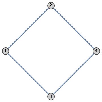
As we can see there is no edge between the first and the fourth vertices, where the PCM has missing values and there is no edge between the second and third vertices, where the situation is the same. There is an edge between every other pair, where we have no missing values in the PCM.
We assume that the representing graphs are connected and -regular through our paper, thus we need some definitions to make these concepts clear.
Definition 1 (Connected graph)
In an undirected graph, two vertices and are called connected if the graph contains a path from to . A graph is said to be connected if every pair of vertices in the graph is connected.
Definition 2 (-regular graph)
A graph is called -regular if every vertex has neighbours, which means that the degree of every vertex is .
Definition 3 (-quasi-regular graph)
A graph is called -quasi-regular if exactly one vertex has degree , and all the other vertices have degree .
The -regularity basically means that the vertices are not distinguished, there is no particular vertex as, for example, in the case of the star graph, thus we would like to avoid the cases when the elimination of relatively few vertices would lead to the disintegration of the whole comparison system (Tekile, 2017). While the connectedness is really important, because to approximate the decision makers’ preferences well, we need to have at least indirect comparisons between the different criteria, otherwise we cannot say anything about the relation between certain elements.
However, it is also notable that we would like to avoid the cases when two items are compared only indirectly through a very long path, because this could aggregate the small, tolerable errors of the different comparisons and we could end up with an intolerably large error in the relation between the two elements. To measure this problem we can use the diameter of the representing graph:
Definition 4 (The diameter of a graph)
The diameter (denoted by ) of a graph G is the length of the longest shortest path between any two vertices:
where denotes the set of vertices of and is the graph distance between two vertices, namely the length of the shortest path between them.
Briefly from now on we will examine graphs representing MCDM problems defined by the following inputs: , where is the number of vertices (criteria), shows the level of regularity of the graph and is the diameter of the graph.
3 Results
First of all it is a key step to determine which cases are interesting for us considering our inputs. It is important to emphasize that we deal with unlabelled graphs, because we are trying to find out what kind of patterns are needed in the comparisons for different instances, thus if we exchange the ’names’ of two criteria (like if we would change ’1’ and ’2’ in Example 1) the pattern would be the same.
Then we can consider the regularity parameter, . The case is possible only when is even, but they are not connected except for , so this is not really interesting for us. When there is only one connected graph for every , namely the cycle, for which as already mentioned in the introduction.
The larger regularity parameters could be interesting for us, but of course we need a reasonable upper bound for the number of criteria, , which is also an indirect upper bound for . In our research we examined the cases, because in the one hand for larger parameters, some computations become really difficult, and in the other hand we think that it is reasonable to assume that we do not have more than 20 important criteria or 20 relatively good alternatives in most of the MCDM problems.
The smaller the parameter is, the more stable or the more trustworthy our system of comparisons is. This means that in an optimal case we would like to minimize this parameter, while the number of the criteria () is always a given exogenous parameter in our MCDM problems. As we mentioned above, is crucial to avoid the cases when some criteria (vertices) would be too important in the system, however it also shows us how many comparisons have to be made, because every vertex has a degree of , which means the number of edges is . Thus if our decision makers would like to spend the shortest time with the creation of the PCM, we should choose a small parameter. But, of course, as usually happens in these situations, there is a trade off between the parameters, because for many criteria (large ) the smaller regularity () will cause a bigger diameter (), namely a more fragile system of comparisons.
In this paper we would like to provide a list of graphs which shows the patterns of the comparisons that have to be made in case of different parameters. We used an algorithm which defines the graph(s) with the smallest diameter ( parameter) for a given pair. With the help of these results it was easy to determine which is the smallest that is needed to reach a given for a given . We found that, with the chosen upper bound of (20) the interesting values for the regularity are , while the interesting values for the diameter of the graph are . For a general MCDM problem probably instead of , it would give more information if we considered an indicator that shows how far we are from the ’extreme’ case when the decision makers have to make all the comparisons. This would mean comparisons instead of our in case of regular graphs or in case of quasi-regular graphs, therefore the completion ratio is defined as follows:
that we will calculate for every instance.
Now we will present the results of the algorithm which gives the graphs with the smallest diameter for a given pair. Of course would mean a complete graph that is not reachable for many pairs, and also not so interesting for us, thus Table 1 shows the cases when and is the minimal value of the parameter. It is also important to note that is only possible when is even, but when it is odd, we examine graphs where all vertices’ degrees are 3 except one where it is 4, because these are the closest to 3-regularity.
| =3 | Graph | Further information | =3 | Graph | Further information |
|---|---|---|---|---|---|
| =5 |
![[Uncaptioned image]](2006.01127v1/5_vertices_example.jpg)
|
• 8/10 comparisons () • graphs | =6 |
![[Uncaptioned image]](2006.01127v1/3_prism_graph.jpg) 3-prism graph
3-prism graph
|
• 9/15 comparisons () • 2 graphs • The other solution is the bipartite graph |
| =7 |
![[Uncaptioned image]](2006.01127v1/7_vertices_example.jpg)
|
• 11/21 comparisons () • graphs | =8 |
![[Uncaptioned image]](2006.01127v1/Wagner_graph.jpg) Wagner graph
Wagner graph
|
• 12/28 comparisons () • 2 graphs |
| =9 |
![[Uncaptioned image]](2006.01127v1/9_vertices_example.jpg)
|
• 14/36 comparisons () • graph | =10 |
![[Uncaptioned image]](2006.01127v1/Petersen_graph.jpg) Petersen graph
Petersen graph
|
• 15/45 comparisons () • Unique graph |
We can see that with the minimal diameter can be 2 until we have 10 vertices. Of course for the 3-regularity is not possible, and for the diameter is 1, because this is a complete graph, but those are really simple (trivial) cases with few possibilities, that is why we skip those in the table. It is also notable that the completion ratio () even reach when we have 10 vertices (it is obviously decreasing in ). And we should emphasize the fact that there are only a few graphs for every pair with the minimal diameter, and one of them is often a bipartite graph that is not the best design in a decision problem, because the two groups are always compared through the other ones (Csató, 2015). Where the table contains ’ graphs’ that means we have not checked all the possible cases with minimal diameter, but in connection with decision making problems it is enough to see that there is one pattern that satisfies the needed properties.
If we go on to larger graphs (), then we will find that the smallest reachable diameter changes to , but it is also true that at first we have so many graphs that satisfies these properties. However as we examine the or the cases, we can see that there is only one graph that fulfils our assumptions (Pratt, 1996). The results in case of larger graphs, with 3-regularity and 3 as the minimal diameter can be found in Table 2.
| =3 | Graph | Further information | =3 | Graph | Further information |
|---|---|---|---|---|---|
| =11 |
![[Uncaptioned image]](2006.01127v1/11_vertices_k_3.jpg)
|
• 17/55 comparisons () • graphs | =12 |
![[Uncaptioned image]](2006.01127v1/Tietze_graph.jpg) Tietze graph
Tietze graph
|
• 18/66 comparisons () • 34 graphs |
| =13 |
![[Uncaptioned image]](2006.01127v1/13_vertices_k_3.jpg)
|
• 20/78 comparisons () • graphs | =14 |
![[Uncaptioned image]](2006.01127v1/Heawood_graph.jpg) Heawood graph
Heawood graph
|
• 21/91 comparisons () • 34 graphs |
| =15 |
![[Uncaptioned image]](2006.01127v1/15_vertices_k_3.jpg)
|
• 23/105 comparisons () • graphs | =16 |
![[Uncaptioned image]](2006.01127v1/16_vertices_example.jpg)
|
• 24/120 comparisons () • 14 graphs |
| =17 |
![[Uncaptioned image]](2006.01127v1/17_vertices_k_3.jpg)
|
• 26/136 comparisons () • graph | =18 |
![[Uncaptioned image]](2006.01127v1/18_vertices_3_3_graph.jpg) (3,3) graph on 18 vertices
(3,3) graph on 18 vertices
|
• 27/153 comparisons () • Unique graph |
| =19 |
![[Uncaptioned image]](2006.01127v1/19_vertices_k_3.jpg)
|
• 29/171 comparisons ( • graph | =20 |
![[Uncaptioned image]](2006.01127v1/20_3_3_graph.jpg) (3,3)-graph on 20 vertices (C5xF4)
(3,3)-graph on 20 vertices (C5xF4)
|
• 30/190 comparisons ( • Unique graph |
As we can see the completion ratio is still decreasing in and on larger graphs it can be taken below 0.2. It is also true that we still do not need to answer for more than 30 questions for an MCDM problem with 20 criteria, which can be really useful.
We discussed all the possible cases for and , and we saw that the minimal diameter is 2 or 3 here. We also mentioned that the 1 diameter would mean a complete graph and a complete PCM, so that is not interesting for us. This means that if we would like to examine the graphs where it is obvious that the minimal diameter would be 2 until , but it is not so important to make so many comparisons because this property can be reached with , too. Thus for the interesting cases start above 10 vertices, and the question is that can we reach a smaller diameter (a more stable system of comparisons) with the rise of the answered questions. We found that with we can get 2 as the minimal diameter until , but for larger values of , it will be 3 again which can be also reached by , thus we would not recommend these combinations of parameters. The results for are shown in Table 3. It is also important to note that is possible in case of both odd and even values of , thus now we do not have to pay special attention to this.
| =4 | Graph | Further information |
|---|---|---|
| =11 |
![[Uncaptioned image]](2006.01127v1/4_Andrasfai_graph.jpg) 4-Andrásfai graph
4-Andrásfai graph
|
• 22/55 comparisons () • 37 graphs |
| =12 |
![[Uncaptioned image]](2006.01127v1/Chvatal_graph.jpg) Chvátal graph
Chvátal graph
|
• 24/66 comparisons () • 26 graphs |
| =13 |
![[Uncaptioned image]](2006.01127v1/13_cyclotonic_graph.jpg) 13-cyclotomic graph
13-cyclotomic graph
|
• 26/78 comparisons () • 10 graphs |
| =14 |
![[Uncaptioned image]](2006.01127v1/14_vertices_k_4.jpg) Unique graph on 14 vertices
Unique graph on 14 vertices
|
• 28/91 comparisons () • Unique graph |
| =15 |
![[Uncaptioned image]](2006.01127v1/15_vertices_k_4.jpg) Unique graph on 15 vertices
Unique graph on 15 vertices
|
• 30/105 comparisons () • Unique graph |
As we can see, the completion ratio is increasing in , so we cannot get so small values as in the former table, however the system of comparisons will be more stable even on many vertices, because the smallest diameter is 2 here. It is also really interesting that, for larger graphs and regularity levels, the number of connected graphs increase very rapidly. For instance, when we have 15 vertices, there are 805 491 connected 4-regular graphs (that means 805 491 possible filling patterns of the PCM), and only one has 2 as its diameter. Our algorithms and methodology has a strong relationship with the so-called degree-diameter problem that is well known in the literature of mathematics (Dinneen and Hafner, 1994, Loz and Sirán, 2008), but they are looking for the largest possible for a given diameter and a given level of regularity. The scientific results in this field support our findings, too, because for the largest is 10, while for it is 20. In the case of the largest is 15, but for it is proved that the largest graph is much above our bound, but the optimal number of the vertices in this case is still an open question.
Finally, we can increase the regularity level to 5 in order to find out if we are able to get 2 as the smallest diameter for larger graphs. The answer is yes, actually it is also proven that is reachable for 5-regular graphs until 24 vertices, but of course we are interested in the specific graphs that could help us determine the adequate comparison patterns. Our results can be found in Table 4. The parameter is only possible when is even again, so when it is odd, we let one vertex have 6 as its degree.
| =5 | Graph | Further information |
|---|---|---|
| =16 |
![[Uncaptioned image]](2006.01127v1/Clebsch_graph.jpg) Clebsch graph
Clebsch graph
|
• 40/120 comparisons () • graphs |
| =17 |
![[Uncaptioned image]](2006.01127v1/17_vertices_k_5.jpg)
|
• 43/136 comparisons () • graph |
| =18 |
![[Uncaptioned image]](2006.01127v1/18_1_noncayley_transitive_graph.jpg) (18,1)-noncayley transitive graph
(18,1)-noncayley transitive graph
|
• 45/153 comparisons () • graph |
| =19 |
![[Uncaptioned image]](2006.01127v1/19_vertices_k_5.jpg)
|
• 48/171 comparisons () • graph |
| =20 |
![[Uncaptioned image]](2006.01127v1/20_8_noncayley_transitive_graph.jpg) (20,8)-noncayley transitive graph
(20,8)-noncayley transitive graph
|
• 50/190 comparisons () • graph |
As we can see in this table there are higher completion ratios again, and for instance when we have 20 vertices the decision makers should make 50 comparisons which in certain situations can be too many. One can also note that in this table we report that there are some graphs with the needed properties, but never indicate the number of them. The reason behind this is simple: the really high number of the potential connected 5-regular graphs (for instance in the case of there are roughly possibilities).
This means that we have examined all the cases that we previously called interesting. According to our results if we use the parameters, then for smaller MCDM problems the is enough to get 2 as the diameter of the representing graph which leads to a small completion ratio and a stable system of the comparisons. In larger problems, when we have more alternatives or criteria we can choose if we use , when the completion ratio is smaller, but our approximation can be unstable, or choose higher regularity levels with more reliable results but a higher completion ratio. We also showed examples and graphs with the needed properties for the different cases, which can help anyone in a MCDM problem to decide which comparisons have to be made. One can find the summary of our results in Table 5, which shows how many graphs we know for given parameters. It is also true that if there is a graph for in the table, then there are graphs for too, where , and there is no graph with the parameters of . We omitted the cases when and , because the minimal diameter is the same as it was in the case of . There is the same reasoning behind the emptiness of the table when and . We have not included the cases when and , because can be reached by -regular graphs, but for at least -regularity is needed.
![[Uncaptioned image]](2006.01127v1/osszegzo.jpg)
4 Conclusion and further research
In this article we provided a systematic collection of recommended filling patterns of incomplete pairwise comparisons’ using the graph representation of the PCMs. We discussed the applied methodology in many details, and then presented our results using the number of criteria or alternatives, the regularity level and the diameter of the representing graph as parameters. We showed that relatively small completion ratios can be achieved with small diameters, and provided examples for every case that we considered to be relevant.
The investigation of the robustness of the results, namely what is between the different regularity levels, could be the topic of a further research. It is also an interesting problem to concentrate directly on the completion ratio as a parameter instead of the regularity of the representing graph. If the pair is given then what comparisons are the most important to be made? We would like to deal with these questions in our future works.
Although our results have been presented within the framework of pairwise comparison matrices, they are applicable in a wider range. A lot of other models based on pairwise comparisons can utilize our findings. For example ranking of sport players or teams based on their matches leads to the problem of tournament design: which pairs should play against each other?
References
- Blanquero et al., (2006) Blanquero, R., Carrizosa, E., and Conde, E. (2006). Inferring efficient weights from pairwise comparison matrices. Mathematical Methods of Operations Research, 64(2):271–284.
- Bozóki et al., (2016) Bozóki, S., Csató, L., and Temesi, J. (2016). An application of incomplete pairwise comparison matrices for ranking top tennis players. European Journal of Operational Research, 248(1):211–218.
- Csató, (2013) Csató, L. (2013). Ranking by pairwise comparisons for swiss-system tournaments. Central European Journal of Operations Research, 21:783–803.
- Csató, (2015) Csató, L. (2015). A graph interpretation of the least squares ranking method. Social Choice and Welfare, 44(1):51–69.
- Dinneen and Hafner, (1994) Dinneen, M. J. and Hafner, P. R. (1994). New results for the degree/diameter problem. Networks, 24(7):359–367.
- Gass, (1998) Gass, S. I. (1998). Tournaments, transitivity and pairwise comparison matrices. The Journal of the Operational Research Society, 49(6):616–624.
- Kendall and Smith, (1940) Kendall, M. G. and Smith, B. B. (1940). On the method of paired comparisons. Biometrika, 31(3/4):324–345.
- Loz and Sirán, (2008) Loz, E. and Sirán, J. (2008). New record graphs in the degree-diameter problem. Australasian Journal of Combinatorics, 41:63–80.
- Pratt, (1996) Pratt, R. W. (1996). The complete catalog of 3-regular, diameter-3 planar graphs.
- Rezaei, (2015) Rezaei, J. (2015). Best-worst multi-criteria decision-making method. Omega, 53:49–57.
- Saaty, (1980) Saaty, T. L. (1980). The Analytic Hierarchy Process. McGraw-Hill, New York.
- Tekile, (2017) Tekile, H. A. (2017). Incomplete pairwise comparison matrices in multi-criteria decision making and ranking. MSc Thesis, Central European University.
5 Appendix1: and graphs

’Graph6’ format: ␣D}k
| 1 | 2 | 3 | 4 | 5 | |
| 1 | |||||
| 2 | |||||
| 3 | |||||
| 4 | |||||
| 5 |
Edges
1-2
1-3
1-4
1-5
2-3
2-4
3-5
4-5

’Graph6’ format: ␣E{Sw
| 1 | 2 | 3 | 4 | 5 | 6 | |
| 1 | ||||||
| 2 | ||||||
| 3 | ||||||
| 4 | ||||||
| 5 | ||||||
| 6 |
Edges
1-2
1-3
1-4
2-3
2-5
3-6
4-5
4-6
5-6

’Graph6’ format: ␣FsdrO
| 1 | 2 | 3 | 4 | 5 | 6 | 7 | |
| 1 | |||||||
| 2 | |||||||
| 3 | |||||||
| 4 | |||||||
| 5 | |||||||
| 6 | |||||||
| 7 |
Edges
1-2
1-3
1-4
1-7
2-5
2-6
3-5
3-6
4-5
4-7
6-7

’Graph6’ format: ␣GhdHKc
| 1 | 2 | 3 | 4 | 5 | 6 | 7 | 8 | |
| 1 | ||||||||
| 2 | ||||||||
| 3 | ||||||||
| 4 | ||||||||
| 5 | ||||||||
| 6 | ||||||||
| 7 | ||||||||
| 8 |
Edges
1-2
1-5
1-8
2-3
2-6
3-4
3-7
4-5
4-8
5-6
6-7
7-8

’Graph6’ format: ␣HsT@PWU
| 1 | 2 | 3 | 4 | 5 | 6 | 7 | 8 | 9 | |
| 1 | |||||||||
| 2 | |||||||||
| 3 | |||||||||
| 4 | |||||||||
| 5 | |||||||||
| 6 | |||||||||
| 7 | |||||||||
| 8 | |||||||||
| 9 |
Edges
1-2
1-4
1-5
2-3
2-6
3-4
3-7
3-8
4-9
5-7
5-8
6-8
6-9
7-9

’Graph6’ format: ␣IUYAHCPBG
| 1 | 2 | 3 | 4 | 5 | 6 | 7 | 8 | 9 | 10 | |
| 1 | ||||||||||
| 2 | ||||||||||
| 3 | ||||||||||
| 4 | ||||||||||
| 5 | ||||||||||
| 6 | ||||||||||
| 7 | ||||||||||
| 8 | ||||||||||
| 9 | ||||||||||
| 10 |
Edges
1-3
1-4
1-6
2-4
2-5
2-7
3-5
3-8
4-9
5-10
6-7
6-10
7-8
8-9
9-10
6 Appendix2: and graphs

’Graph6’ format: ␣J{COXCPAIG_
| 1 | 2 | 3 | 4 | 5 | 6 | 7 | 8 | 9 | 10 | 11 | |
| 1 | |||||||||||
| 2 | |||||||||||
| 3 | |||||||||||
| 4 | |||||||||||
| 5 | |||||||||||
| 6 | |||||||||||
| 7 | |||||||||||
| 8 | |||||||||||
| 9 | |||||||||||
| 10 | |||||||||||
| 11 |
Edges
1-2
1-3
1-4
2-3
2-10
3-7
4-5
4-8
4-11
5-6
5-9
6-7
6-11
7-8
8-9
9-10
10-11

’Graph6’ format: ␣KhDGHEH_?__R
| 1 | 2 | 3 | 4 | 5 | 6 | 7 | 8 | 9 | 10 | 11 | 12 | |
| 1 | ||||||||||||
| 2 | ||||||||||||
| 3 | ||||||||||||
| 4 | ||||||||||||
| 5 | ||||||||||||
| 6 | ||||||||||||
| 7 | ||||||||||||
| 8 | ||||||||||||
| 9 | ||||||||||||
| 10 | ||||||||||||
| 11 | ||||||||||||
| 12 |
Edges
1-2
1-9
1-10
2-3
2-6
3-4
3-8
4-5
4-11
5-6
5-9
6-7
7-8
7-12
8-9
10-11
10-12
11-12

’Graph6’ format: ␣LhcIGCP_GGc@_P
| 1 | 2 | 3 | 4 | 5 | 6 | 7 | 8 | 9 | 10 | 11 | 12 | 13 | |
| 1 | |||||||||||||
| 2 | |||||||||||||
| 3 | |||||||||||||
| 4 | |||||||||||||
| 5 | |||||||||||||
| 6 | |||||||||||||
| 7 | |||||||||||||
| 8 | |||||||||||||
| 9 | |||||||||||||
| 10 | |||||||||||||
| 11 | |||||||||||||
| 12 | |||||||||||||
| 13 |
Edges
1-2
1-5
1-10
1-13
2-3
2-7
3-4
3-12
4-5
4-9
5-6
6-7
6-11
7-8
8-9
8-13
9-10
10-11
11-12
12-13

’Graph6’ format: ␣MhEGHC@AI?_PC@_G_
| 1 | 2 | 3 | 4 | 5 | 6 | 7 | 8 | 9 | 10 | 11 | 12 | 13 | 14 | |
| 1 | ||||||||||||||
| 2 | ||||||||||||||
| 3 | ||||||||||||||
| 4 | ||||||||||||||
| 5 | ||||||||||||||
| 6 | ||||||||||||||
| 7 | ||||||||||||||
| 8 | ||||||||||||||
| 9 | ||||||||||||||
| 10 | ||||||||||||||
| 11 | ||||||||||||||
| 12 | ||||||||||||||
| 13 | ||||||||||||||
| 14 |
Edges
1-2
1-6
1-14
2-3
2-11
3-4
3-8
4-5
4-13
5-6
5-10
6-7
7-8
7-12
8-9
9-10
9-14
10-11
11-12
12-13
13-14

’Graph6’ format: ␣N{O___GA?G?k?i?d?J?
| 1 | 2 | 3 | 4 | 5 | 6 | 7 | 8 | 9 | 10 | 11 | 12 | 13 | 14 | 15 | |
| 1 | |||||||||||||||
| 2 | |||||||||||||||
| 3 | |||||||||||||||
| 4 | |||||||||||||||
| 5 | |||||||||||||||
| 6 | |||||||||||||||
| 7 | |||||||||||||||
| 8 | |||||||||||||||
| 9 | |||||||||||||||
| 10 | |||||||||||||||
| 11 | |||||||||||||||
| 12 | |||||||||||||||
| 13 | |||||||||||||||
| 14 | |||||||||||||||
| 15 |
Edges
1-2
1-3
1-4
2-3
2-5
3-6
4-7
4-8
5-9
5-10
6-11
6-12
7-13
7-14
8-12
8-15
9-12
9-13
10-14
10-15
11-13
11-15
12-14

’Graph6’ format: ␣O{O___GA?G?_?i?d?K_Ao
| 1 | 2 | 3 | 4 | 5 | 6 | 7 | 8 | 9 | 10 | 11 | 12 | 13 | 14 | 15 | 16 | |
| 1 | ||||||||||||||||
| 2 | ||||||||||||||||
| 3 | ||||||||||||||||
| 4 | ||||||||||||||||
| 5 | ||||||||||||||||
| 6 | ||||||||||||||||
| 7 | ||||||||||||||||
| 8 | ||||||||||||||||
| 9 | ||||||||||||||||
| 10 | ||||||||||||||||
| 11 | ||||||||||||||||
| 12 | ||||||||||||||||
| 13 | ||||||||||||||||
| 14 | ||||||||||||||||
| 15 | ||||||||||||||||
| 16 |
Edges
1-2
1-3
1-4
2-3
2-5
3-6
4-7
4-8
5-9
5-10
6-11
6-12
7-13
7-14
8-15
8-16
9-13
9-15
10-14
10-16
11-13
11-16
12-14
12-15

’Graph6’ format: ␣PhCGKCH?K?_PG@?Cg?GG@c?C
| 1 | 2 | 3 | 4 | 5 | 6 | 7 | 8 | 9 | 10 | 11 | 12 | 13 | 14 | 15 | 16 | 17 | |
| 1 | |||||||||||||||||
| 2 | |||||||||||||||||
| 3 | |||||||||||||||||
| 4 | |||||||||||||||||
| 5 | |||||||||||||||||
| 6 | |||||||||||||||||
| 7 | |||||||||||||||||
| 8 | |||||||||||||||||
| 9 | |||||||||||||||||
| 10 | |||||||||||||||||
| 11 | |||||||||||||||||
| 12 | |||||||||||||||||
| 13 | |||||||||||||||||
| 14 | |||||||||||||||||
| 15 | |||||||||||||||||
| 16 | |||||||||||||||||
| 17 |
Edges
1-2
1-8
1-11
1-17
2-3
2-15
3-4
3-13
4-5
4-17
5-6
5-9
6-7
6-16
7-8
7-12
8-9
9-10
10-11
10-14
11-12
12-13
13-14
14-15
15-16
16-17

’Graph6’ format: ␣QhCGKCH?G?_PG@?Cg?GG@C?E?GG
| 1 | 2 | 3 | 4 | 5 | 6 | 7 | 8 | 9 | 10 | 11 | 12 | 13 | 14 | 15 | 16 | 17 | 18 | |
| 1 | ||||||||||||||||||
| 2 | ||||||||||||||||||
| 3 | ||||||||||||||||||
| 4 | ||||||||||||||||||
| 5 | ||||||||||||||||||
| 6 | ||||||||||||||||||
| 7 | ||||||||||||||||||
| 8 | ||||||||||||||||||
| 9 | ||||||||||||||||||
| 10 | ||||||||||||||||||
| 11 | ||||||||||||||||||
| 12 | ||||||||||||||||||
| 13 | ||||||||||||||||||
| 14 | ||||||||||||||||||
| 15 | ||||||||||||||||||
| 16 | ||||||||||||||||||
| 17 | ||||||||||||||||||
| 18 |
Edges
1-2
1-8
1-18
2-3
2-15
3-4
3-13
4-5
4-17
5-6
5-9
6-7
6-16
7-8
7-12
8-9
9-10
10-11
10-14
11-12
11-18
12-13
13-14
14-15
15-16
16-17
17-18

’Graph6’ format: ␣RhECQ?_@G¿@@?C?_G_AO?_S?_G?DG
| 1 | 2 | 3 | 4 | 5 | 6 | 7 | 8 | 9 | 10 | 11 | 12 | 13 | 14 | 15 | 16 | 17 | 18 | 19 | |
| 1 | |||||||||||||||||||
| 2 | |||||||||||||||||||
| 3 | |||||||||||||||||||
| 4 | |||||||||||||||||||
| 5 | |||||||||||||||||||
| 6 | |||||||||||||||||||
| 7 | |||||||||||||||||||
| 8 | |||||||||||||||||||
| 9 | |||||||||||||||||||
| 10 | |||||||||||||||||||
| 11 | |||||||||||||||||||
| 12 | |||||||||||||||||||
| 13 | |||||||||||||||||||
| 14 | |||||||||||||||||||
| 15 | |||||||||||||||||||
| 16 | |||||||||||||||||||
| 17 | |||||||||||||||||||
| 18 | |||||||||||||||||||
| 19 |
Edges
1-2
1-6
1-7
2-3
2-8
3-4
3-9
4-5
4-14
5-7
5-12
6-10
6-13
7-17
8-15
8-16
9-10
9-18
10-11
11-12
11-16
12-15
13-14
13-19
14-17
15-19
16-17
17-18
18-19

’Graph6’ format: ␣ShECQ?_@G¿@@?C?_G_AO?_??@W@?O?DC
| 1 | 2 | 3 | 4 | 5 | 6 | 7 | 8 | 9 | 10 | 11 | 12 | 13 | 14 | 15 | 16 | 17 | 18 | 19 | 20 | |
| 1 | ||||||||||||||||||||
| 2 | ||||||||||||||||||||
| 3 | ||||||||||||||||||||
| 4 | ||||||||||||||||||||
| 5 | ||||||||||||||||||||
| 6 | ||||||||||||||||||||
| 7 | ||||||||||||||||||||
| 8 | ||||||||||||||||||||
| 9 | ||||||||||||||||||||
| 10 | ||||||||||||||||||||
| 11 | ||||||||||||||||||||
| 12 | ||||||||||||||||||||
| 13 | ||||||||||||||||||||
| 14 | ||||||||||||||||||||
| 15 | ||||||||||||||||||||
| 16 | ||||||||||||||||||||
| 17 | ||||||||||||||||||||
| 18 | ||||||||||||||||||||
| 19 | ||||||||||||||||||||
| 20 |
Edges
1-2
1-6
1-7
2-3
2-8
3-4
3-9
4-5
4-14
5-7
5-12
6-10
6-13
7-17
8-15
8-16
9-10
9-19
10-11
11-12
11-16
12-15
13-14
13-20
14-18
15-20
16-18
17-18
17-19
19-20
7 Appendix3: and graphs

’Graph6’ format: ␣JlSggUDOlA_
| 1 | 2 | 3 | 4 | 5 | 6 | 7 | 8 | 9 | 10 | 11 | |
| 1 | |||||||||||
| 2 | |||||||||||
| 3 | |||||||||||
| 4 | |||||||||||
| 5 | |||||||||||
| 6 | |||||||||||
| 7 | |||||||||||
| 8 | |||||||||||
| 9 | |||||||||||
| 10 | |||||||||||
| 11 |
Edges
1-2
1-4
1-9
1-11
2-3
2-5
2-10
3-4
3-16
3-11
4-5
4-7
5-6
5-8
6-7
6-9
7-8
7-10
8-9
8-11
9-10
10-11

’Graph6’ format: ␣KG@LIchdMoV?
| 1 | 2 | 3 | 4 | 5 | 6 | 7 | 8 | 9 | 10 | 11 | 12 | |
| 1 | ||||||||||||
| 2 | ||||||||||||
| 3 | ||||||||||||
| 4 | ||||||||||||
| 5 | ||||||||||||
| 6 | ||||||||||||
| 7 | ||||||||||||
| 8 | ||||||||||||
| 9 | ||||||||||||
| 10 | ||||||||||||
| 11 | ||||||||||||
| 12 |
Edges
1-7
1-10
1-11
1-12
2-3
2-6
2-8
2-11
3-7
3-9
3-12
4-8
4-10
4-11
4-12
5-6
5-9
5-11
5-12
6-7
6-10
7-8
8-9
9-10

’Graph6’ format: ␣LhEIHEPQHGaPaP
| 1 | 2 | 3 | 4 | 5 | 6 | 7 | 8 | 9 | 10 | 11 | 12 | 13 | |
| 1 | |||||||||||||
| 2 | |||||||||||||
| 3 | |||||||||||||
| 4 | |||||||||||||
| 5 | |||||||||||||
| 6 | |||||||||||||
| 7 | |||||||||||||
| 8 | |||||||||||||
| 9 | |||||||||||||
| 10 | |||||||||||||
| 11 | |||||||||||||
| 12 | |||||||||||||
| 13 |
Edges
1-2
1-6
1-9
1-13
2-3
2-7
2-10
3-4
3-8
3-11
4-5
4-9
4-12
5-6
5-10
5-13
6-7
6-11
7-8
7-12
8-9
8-13
9-10
10-11
11-12
12-13

’Graph6’ format: ␣Mo?CB‘gXCw@wDgEc?
| 1 | 2 | 3 | 4 | 5 | 6 | 7 | 8 | 9 | 10 | 11 | 12 | 13 | 14 | |
| 1 | ||||||||||||||
| 2 | ||||||||||||||
| 3 | ||||||||||||||
| 4 | ||||||||||||||
| 5 | ||||||||||||||
| 6 | ||||||||||||||
| 7 | ||||||||||||||
| 8 | ||||||||||||||
| 9 | ||||||||||||||
| 10 | ||||||||||||||
| 11 | ||||||||||||||
| 12 | ||||||||||||||
| 13 | ||||||||||||||
| 14 |
Edges
1-2
1-3
1-7
1-11
2-8
2-9
2-10
3-8
3-9
3-10
4-8
4-11
4-13
4-14
5-9
5-11
5-12
5-14
6-10
6-11
6-12
6-13
7-12
7-13
7-14
8-12
9-13
10-14

’Graph6’ format: ␣N?ACE‘cL?wTGEgQcKP?
| 1 | 2 | 3 | 4 | 5 | 6 | 7 | 8 | 9 | 10 | 11 | 12 | 13 | 14 | 15 | |
| 1 | |||||||||||||||
| 2 | |||||||||||||||
| 3 | |||||||||||||||
| 4 | |||||||||||||||
| 5 | |||||||||||||||
| 6 | |||||||||||||||
| 7 | |||||||||||||||
| 8 | |||||||||||||||
| 9 | |||||||||||||||
| 10 | |||||||||||||||
| 11 | |||||||||||||||
| 12 | |||||||||||||||
| 13 | |||||||||||||||
| 14 | |||||||||||||||
| 15 |
Edges
1-6
1-7
1-8
1-12
2-8
2-9
2-14
2-15
3-9
3-10
3-12
3-15
4-8
4-10
4-11
4-13
5-11
5-12
5-13
5-14
6-9
6-10
6-11
7-13
7-14
7-15
8-12
9-13
10-14
11-15
8 Appendix4: and graphs

’Graph6’ format: ␣OPtcIcSoGT@__XWAcJ_ci
| 1 | 2 | 3 | 4 | 5 | 6 | 7 | 8 | 9 | 10 | 11 | 12 | 13 | 14 | 15 | 16 | |
| 1 | ||||||||||||||||
| 2 | ||||||||||||||||
| 3 | ||||||||||||||||
| 4 | ||||||||||||||||
| 5 | ||||||||||||||||
| 6 | ||||||||||||||||
| 7 | ||||||||||||||||
| 8 | ||||||||||||||||
| 9 | ||||||||||||||||
| 10 | ||||||||||||||||
| 11 | ||||||||||||||||
| 12 | ||||||||||||||||
| 13 | ||||||||||||||||
| 14 | ||||||||||||||||
| 15 | ||||||||||||||||
| 16 |
Edges
1-3
1-5
1-7
1-10
1-13
2-5
2-6
2-8
2-10
2-14
3-4
3-6
3-14
3-15
4-5
4-8
4-9
4-16
5-11
5-12
6-7
6-9
6-12
7-8
7-11
7-16
8-13
8-15
9-10
9-11
9-13
10-15
10-16
11-14
11-15
12-13
12-15
12-16
13-14
14-16

’Graph6’ format: ␣PxCYHEBCIO_bGPagiAOQP‘@K
| 1 | 2 | 3 | 4 | 5 | 6 | 7 | 8 | 9 | 10 | 11 | 12 | 13 | 14 | 15 | 16 | 17 | |
| 1 | |||||||||||||||||
| 2 | |||||||||||||||||
| 3 | |||||||||||||||||
| 4 | |||||||||||||||||
| 5 | |||||||||||||||||
| 6 | |||||||||||||||||
| 7 | |||||||||||||||||
| 8 | |||||||||||||||||
| 9 | |||||||||||||||||
| 10 | |||||||||||||||||
| 11 | |||||||||||||||||
| 12 | |||||||||||||||||
| 13 | |||||||||||||||||
| 14 | |||||||||||||||||
| 15 | |||||||||||||||||
| 16 | |||||||||||||||||
| 17 |
Edges
1-2
1-3
1-9
1-14
1-17
2-3
2-7
2-11
2-15
3-4
3-8
3-13
4-5
4-6
4-10
4-15
5-6
5-11
5-14
5-16
6-7
6-12
6-17
7-8
7-9
7-14
8-9
8-13
8-16
9-10
9-14
10-11
10-12
10-15
11-12
11-16
12-13
12-17
13-14
13-15
15-16
15-17
16-17

’Graph6’ format: ␣Q{eAaSqIWI?o@D@IG?X?WCAkGDo
| 1 | 2 | 3 | 4 | 5 | 6 | 7 | 8 | 9 | 10 | 11 | 12 | 13 | 14 | 15 | 16 | 17 | 18 | |
| 1 | ||||||||||||||||||
| 2 | ||||||||||||||||||
| 3 | ||||||||||||||||||
| 4 | ||||||||||||||||||
| 5 | ||||||||||||||||||
| 6 | ||||||||||||||||||
| 7 | ||||||||||||||||||
| 8 | ||||||||||||||||||
| 9 | ||||||||||||||||||
| 10 | ||||||||||||||||||
| 11 | ||||||||||||||||||
| 12 | ||||||||||||||||||
| 13 | ||||||||||||||||||
| 14 | ||||||||||||||||||
| 15 | ||||||||||||||||||
| 16 | ||||||||||||||||||
| 17 | ||||||||||||||||||
| 18 |
Edges
1-2
1-3
1-4
1-5
1-6
2-3
2-7
2-8
2-15
3-9
3-10
3-16
4-5
4-7
4-9
4-17
5-8
5-10
5-18
6-11
6-12
6-13
6-14
7-8
7-9
7-12
8-10
8-11
9-10
9-14
10-13
11-14
11-16
11-17
12-13
12-16
12-18
13-15
13-17
14-15
14-18
15-17
15-18
16-17
16-18

’Graph6’ format: ␣RzAKQQPD@AbOI?O_?Z?IK@BO?rO@FO
| 1 | 2 | 3 | 4 | 5 | 6 | 7 | 8 | 9 | 10 | 11 | 12 | 13 | 14 | 15 | 16 | 17 | 18 | 19 | |
| 1 | |||||||||||||||||||
| 2 | |||||||||||||||||||
| 3 | |||||||||||||||||||
| 4 | |||||||||||||||||||
| 5 | |||||||||||||||||||
| 6 | |||||||||||||||||||
| 7 | |||||||||||||||||||
| 8 | |||||||||||||||||||
| 9 | |||||||||||||||||||
| 10 | |||||||||||||||||||
| 11 | |||||||||||||||||||
| 12 | |||||||||||||||||||
| 13 | |||||||||||||||||||
| 14 | |||||||||||||||||||
| 15 | |||||||||||||||||||
| 16 | |||||||||||||||||||
| 17 | |||||||||||||||||||
| 18 | |||||||||||||||||||
| 19 |
Edges
1-2
1-3
1-6
1-7
1-9
2-3
2-4
2-8
2-14
3-4
3-11
3-13
4-9
4-10
4-12
5-6
5-7
5-8
5-12
5-13
6-10
6-16
6-17
7-12
7-14
7-15
8-9
8-15
8-16
8-11
9-18
9-19
10-11
10-15
10-18
11-15
11-17
12-16
12-17
13-16
13-18
13-19
14-17
14-18
14-19
15-19
16-18
17-19

’Graph6’ format: ␣Ssa@Gt‘PQcHOGCGC?cOHAC@cOD_OSgORO
| 1 | 2 | 3 | 4 | 5 | 6 | 7 | 8 | 9 | 10 | 11 | 12 | 13 | 14 | 15 | 16 | 17 | 18 | 19 | 20 | |
| 1 | ||||||||||||||||||||
| 2 | ||||||||||||||||||||
| 3 | ||||||||||||||||||||
| 4 | ||||||||||||||||||||
| 5 | ||||||||||||||||||||
| 6 | ||||||||||||||||||||
| 7 | ||||||||||||||||||||
| 8 | ||||||||||||||||||||
| 9 | ||||||||||||||||||||
| 10 | ||||||||||||||||||||
| 11 | ||||||||||||||||||||
| 12 | ||||||||||||||||||||
| 13 | ||||||||||||||||||||
| 14 | ||||||||||||||||||||
| 15 | ||||||||||||||||||||
| 16 | ||||||||||||||||||||
| 17 | ||||||||||||||||||||
| 18 | ||||||||||||||||||||
| 19 | ||||||||||||||||||||
| 20 |
Edges
1-2
1-3
1-4
1-5
1-6
2-9
2-10
2-11
2-12
3-7
3-9
3-13
3-14
4-8
4-11
4-17
4-18
5-8
5-12
5-19
5-20
6-7
6-10
6-15
6-16
7-8
7-11
7-12
8-9
8-10
9-15
9-16
10-13
10-14
11-19
11-20
12-17
12-18
13-15
13-17
13-19
14-16
14-18
14-20
15-18
15-20
16-17
16-19
17-20
18-19