Hadamard Wirtinger Flow for Sparse Phase Retrieval

Phase retrieval, the problem of reconstructing a signal from the (squared) magnitude of its Fourier (or any linear) transform, arises in many fields of science and engineering. Such a task is naturally involved in applications such as crystallography (Millane 1990) and diffraction imaging (Bunk et al. 2007), where optical sensors are able to measure intensities, but not phases of light waves. Due to the loss of phase information, the one-dimensional Fourier phase retrieval problem is ill-posed in general. Common approaches to overcome this ill-posedness include using prior information such as non-negativity, sparsity and the signal’s magnitude (Fienup 1982; Jaganathan et al. 2016), or introducing redundancy into the measurements by oversampling random Gaussian measurements or coded diffraction patterns (Candès et al. 2015; Chen and Candès 2015).

In many applications, the underlying signal is naturally sparse (Jaganathan et al. 2016). A wide range of algorithms has been devised for phase retrieval with a sparse signal, including alternating minimization (SparseAltMinPhase) (Netrapalli et al. 2015), non-convex optimization based approaches such as thresholded Wirtinger flow (TWF) (Cai et al. 2016), sparse truncated amplitude flow (SPARTA) (Wang et al. 2018), compressive reweighted amplitude flow (CRAF) (Zhang et al. 2018) and sparse Wirtinger flow (SWF) (Yuan et al. 2019), and convex relaxation based methods such as compressive phase retrieval via lifting (CPRL) (Ohlsson et al. 2012) and SparsePhaseMax (Hand and Voroninski 2016). Other approaches to sparse phase retrieval include the greedy algorithm GESPAR (Schechtman et al. 2014), a generalized approximate message passing algorithm (PR-GAMP) (Schniter and Rangan 2015) and majorization minimization algorithms (Qiu and Palomar 2017).

A limitation of these algorithms is their sample complexity: the best known theoretical results require $\mathcal{O}(k^{2}\log n)$ Gaussian measurements to guarantee successful reconstruction of a generic $k$-sparse signal $\mathbf{x}^{*}\in\mathbb{R}^{n}$. On the other hand, it has been shown that reconstruction is possible from $\mathcal{O}(k\log n)$ phaseless measurements (Eldar and Mendelson 2014); however, there is no known algorithm which provably achieves this in polynomial time. In fact, $\mathcal{O}(k^{2}\log n)$ quadratic measurements are necessary for a certain class of convex relaxations, on which algorithms such as CPRL are based (Li and Voroninski 2013). Other existing algorithms such as SPARTA and SparseAltMinPhase require a sample complexity of $\mathcal{O}(k^{2}\log n)$ for the initial estimation of the support of the signal. With the knowledge of the support, these (and plenty other) algorithms require only $\mathcal{O}(k\log n)$ samples for the subsequent reconstruction of the signal. Hence, we identify the support recovery step as the bottleneck of the sample complexity of non-convex optimization based approaches to the sparse phase retrieval problem.

Additional structural assumptions have been considered to improve the sample complexity. It has been shown that a $k$-sparse signal $\mathbf{x}^{*}$ can be reconstructed from $\mathcal{O}(k\log n)$ measurements if one is allowed to freely design the measurement vectors (Jaganathan et al. 2013), or if the signal $\mathbf{x}^{*}$ is assumed to be block-sparse and the number of blocks containing non-zero entries is $\mathcal{O}(1)$ (Jagatap and Hedge 2017; Zhang et al. 2018). However, exact knowledge of the additional structure as well as an algorithm designed to take advantage of it is necessary in both cases. Linear sample complexity has also been achieved assuming that the signal coefficients decay with power-law (Jagatap and Hedge 2019).

Another downside of the above algorithms is the fact that sparsity is enforced or promoted explicitly. For instance, CPRL and SparsePhaseMax augment the objective function with an $\ell_{1}$ penalty term, which is known to promote sparsity. SWF and SPARTA include a thresholding step in their gradient updates, which projects the iterates onto the set of $k$-sparse vectors, and SparseAltMinPhase and GESPAR directly constrain the search to a $k$-dimensional subspace of $\mathbb{R}^{n}$, which needs to be carefully chosen and updated. In the case of CPRL and SparsePhaseMax, additional regularization parameters have to be tuned, while the thresholding step of SWF and SPARTA requires knowledge of the sparsity $k$.

We denote vectors and matrices with boldface letters and real numbers with normal font, and, where appropriate, use uppercase letters for random and lowercase letters for deterministic quantities. For vectors $\mathbf{u},\mathbf{v}\in\mathbb{R}^{n}$ we write $\odot$ for the Hadamard product, $(\mathbf{u}\odot\mathbf{v})_{i}=u_{i}v_{i}$, and, for notational simplicity, $\mathbf{u}^{2}=\mathbf{u}\odot\mathbf{u}$ for taking squares entry-wise. We use the common notation $[n]:=\{1,...,n\}$. Since it is impossible to distinguish $\mathbf{x}^{*}$ from $-\mathbf{x}^{*}$ using magnitude-only observations, we will often write $\mathbf{x}^{*}$ for the solution set $\{\pm\mathbf{x}^{*}\}$ and consider, for any $\mathbf{x}\in\mathbb{R}^{n}$, the distance $\operatorname{dist}(\mathbf{x},\mathbf{x}^{*}):=\min\{\|\mathbf{x}-\mathbf{x}^{*}\|_{2},\|\mathbf{x}+\mathbf{x}^{*}\|_{2}\}$. Further, we assume $\|\mathbf{x}^{*}\|_{2}=1$ for notational simplicity; note that this assumption is not needed for our results.

The goal in phase retrieval is to reconstruct an unknown signal vector $\mathbf{x}^{*}\in\mathbb{R}^{n}$ from a set of quadratic measurements $Y_{j}=(\mathbf{A}_{j}^{T}\mathbf{x}^{*})^{2}$, $j=1,...,m,$ where we observe $\mathbf{A}_{j}\sim\mathcal{N}(0,\mathbf{I}_{n})$ i.i.d.. For the sake of clarity, we focus on the real-valued model. Our proposed algorithm also works in the complex-valued Gaussian model, where $\mathbf{x}^{*}\in\mathbb{C}^{n}$ and $\mathbf{A}_{j}\sim\mathcal{N}(0,\frac{1}{2}\mathbf{I}_{n})+i\mathcal{N}(0,\frac{1}{2}\mathbf{I}_{n})$.

Many methods have been devised to solve this problem. A popular class of algorithms performs alternating projections onto different constraint sets; these include the seminal error reduction algorithm proposed by Gerchberg and Saxton 1972 and alternating minimization (AltMinPhase) (Netrapalli et al. 2015). Another more recent approach is based on non-convex optimization: Wirtinger flow (WF) (Candès et al. 2015) and its variants (Chen and Candès 2015; Zhang et al. 2017), truncated amplitude flow (TAF) (Wang et al. 2017) and the trust region method of (Sun et al. 2018) all minimize the empirical risk (which is non-convex due to the missing phase) based on different loss functions. The convex alternatives typically use matrix-lifting as in PhaseLift (Candès and Li 2012; Candès et al. 2013) and PhaseCut (Waldspurger et al. 2015), which allows phase retrieval to be formulated as a semidefinite programming problem, or consider a non-lifting convex relaxation and solve the dual problem as in PhaseMax (Goldstein and Studer 2018).

Our approach for estimating the signal $\mathbf{x}^{*}$ follows the established approach of empirical risk minimization. Writing $\mathbf{z}=(y,\mathbf{a})\in\mathbb{R}\times\mathbb{R}^{n}$ for an observation, we consider the loss function $\ell(\mathbf{x},\mathbf{z})=\frac{1}{4}((\mathbf{a}^{T}\mathbf{x})^{2}-y)^{2}$ and, given samples $\mathbf{Z}_{1},...,\mathbf{Z}_{m}$, the empirical risk

It is worth mentioning that in previous applications the amplitude-based loss function $\ell(\mathbf{x},\mathbf{z})=\frac{1}{2}(|\mathbf{a}^{T}\mathbf{x}|-\sqrt{y})^{2}$ has been numerically shown to be more effective in terms of sample complexity than the loss function based on squared magnitudes (Wang et al. 2017; Zhang et al. 2017; Wang et al. 2018). However, with our parametrization, we found the squared magnitude-based loss function to be more effective.

Without any restrictions on the signal $\mathbf{x}^{*}\in\mathbb{R}^{n}$, $2n-1$ Gaussian measurements suffice for $\mathbf{x}^{*}$ to be the unique (up to global sign) minimizer of $F(\mathbf{x})$ with high probability (Balan et al. 2006). If $\mathbf{x}^{*}$ is $k$-sparse, then it has been shown in (Li and Voroninski 2013) that

holds with high probability if we have $m\geq 4k-1$ Gaussian measurements.

Solving (2) involves two main difficulties: $(i)$ the objective function $F$ is non-convex with potentially many local minima and saddle points, and $(ii)$ due to the constraint $\|\mathbf{x}\|_{0}\leq k$ the problem is of combinatorial nature and NP-hard in general.

Regarding the first difficulty, the non-convexity is typically addressed by using a spectral or orthogonality-promoting initialization, which produces an initial estimate close to $\mathbf{x}^{*}$ and in a region where the the objective function is locally strongly convex, leading to linear convergence towards $\mathbf{x}^{*}$ (Candès et al. 2015; Chen and Candès 2015; Wang et al. 2017; Zhang et al. 2017). Recently, it has been shown that such an initialization is not always necessary in the phase retrieval problem and that a random initialization can be used instead (Sun et al. 2018; Chen et al. 2019).

Addressing the second difficulty, an approach replacing the constraint $\|\mathbf{x}\|_{0}\leq k$ in (2) by adding a penalty term $\lambda\|\mathbf{x}\|_{1}$ was proposed in (Yang et al. 2013). However, this procedure requires tuning of the regularization parameter $\lambda$ to reach a desired sparsity level, and it is tailored for Fourier measurements only (in particular, it uses the fact that the DFT matrix is unitary). Recently, methods enforcing the constraint $\|\mathbf{x}\|_{0}\leq k$ via a hard-thresholding step have received a lot of attention. These include SPARTA (Wang et al. 2018), CRAF (Zhang et al. 2018) and SWF (Yuan et al. 2019). However, the implementation of such a thresholding step requires knowledge of $k$ (or a suitable upper bound).

Our proposed method does not have to deal with these difficulties. We also approach the problem by minimizing the objective $F(\mathbf{x})$. However, unlike existing algorithms, we do not need to add any penalty term to the objective or to introduce a thresholding step to enforce the constraint $\|\mathbf{x}\|_{0}\leq k$. Our simulations show that the iterates of gradient descent with Hadamard parametrization remain (approximately) in the low-dimensional space of sparse vectors. Hence, we neither need to tune any regularization parameters, nor do we need knowledge of the underlying signal sparsity. Further, HWF does not need the sophisticated initialization scheme commonly used in non-convex optimization based approaches to (sparse) phase retrieval.

Consider the parametrization $\mathbf{x}=\mathbf{u}\odot\mathbf{u}-\mathbf{v}\odot\mathbf{v}$. Such a parametrization has previously been applied to problems such as sparse recovery (Hoff 2017; Vaškevičius et al. 2019; Zhao et al. 2019) and matrix factorization (Gunasekar et al. 2017; Li et al. 2018; Arora et al. 2019). Exploiting the restricted isometry property (RIP) assumed for these problems, the Hadamard parametrization has been shown to confine the gradient iterates to the low-dimensional spaces of sparse vectors and low-rank matrices, respectively.

Overloading the notation, we write

for the empirical risk, with gradients

and, similarly, $\nabla_{\mathbf{v}}F(\mathbf{u},\mathbf{v})=-2\nabla F(\mathbf{x})\odot\mathbf{v}$. We consider gradient descent in this parametrization,

where we denote by $\mathrm{\textbf{1}}_{n}\in\mathbb{R}^{n}$ the vector of all ones.

The reason why the Hadamard parametrization promotes sparsity is that this parametrization turns the additive updates of gradient descent into multiplicative updates. If we choose a small initialization, then, in the aforementioned problems with RIP assumptions, the multiplicative updates have been shown to lead to off-support variables staying negligibly small while support variables are being fitted. The variables grow exponentially, but at different (time-varying) rates, with off-support variables growing at a smaller rate than support variables. With additive updates, off-support variables would not stay sufficiently small and the algorithm would typically converge towards non-sparse local minima. We provide a more detailed discussion on the role of the Hadamard parametrization in the appendix, which suggests the following initialization:

where we write $\hat{\theta}=(\frac{1}{m}\sum_{j=1}^{m}Y_{j})^{1/2}$ for the estimate of the signal size $\|\mathbf{x}^{*}\|_{2}$ (see e.g. Candès et al. 2015; Wang et al. 2017), $I_{max}=\operatorname{argmax}_{i}\sum_{j=1}^{m}Y_{j}A_{ji}^{2}$ and $\alpha>0$ is the initialization size.

We show in the next section that if $|x^{*}_{I_{max}}|\geq\frac{1}{2}x^{*}_{max}$ and $m$ is sufficiently large, then, with high probability, we can recover the support by running one step of (3). The probability of finding a large coordinate $I_{max}$ can be increased by allowing multiple restarts and considering not only the largest, but also a few more instances in $\{R_{i}\}_{i=1}^{n}:=\{\frac{1}{m}\sum_{j=1}^{m}Y_{j}A_{ji}^{2}\}_{i=1}^{n}$. Specifically, if we allow $\bar{b}$ restarts, we consider different initialization as in (4) using each of the $\bar{b}$ largest instances in $\{R_{i}\}_{i=1}^{n}$. As pointed out in Section 2, $\mathbf{x}^{*}$ is the sparsest minimizer of the objective $F$. Given the results from multiple runs, we can therefore choose the (approximately) sparsest solution, by which we mean the solution where the fewest coordinates make up most (e.g. $95\%$) of the norm $\|\mathbf{X}^{\bar{t}}\|_{2}$. This is summarized in Algorithm 1.

In this section we show, assuming $x^{*}_{min}=\Omega(1/\sqrt{k})$, that one step of Algorithm 1 can be used to recover the support $\mathcal{S}$ from $\mathcal{O}(\max\{k\log n,\,\log^{3}n\}(x^{*}_{max})^{-2})$ Gaussian measurements. As pointed out in Section 2, the sample complexity bottleneck of reconstruction algorithms such as SPARTA and SparseAltMinPhase lies in the initial support recovery. In particular, both algorithms require $\mathcal{O}(k^{2}\log n)$ measurements to guarantee successful support recovery; with the knowledge of the support $\mathcal{S}$, these and plenty other algorithms such as WF, TAF and PhaseLift only require a sample complexity of $\mathcal{O}(k\log n)$ to guaruantee successful reconstruction of a $k$-sparse signal $\mathbf{x}^{*}$.

The main difference from previous work is that we only need a single coordinate $i$ with $|x^{*}_{i}|\geq\frac{1}{2}x^{*}_{max}$ rather than the full support for our initialization. Therefore, our sample complexity depends on $x^{*}_{max}$, which is at least $1/\sqrt{k}$, rather than $x^{*}_{min}$, which can be at most $1/\sqrt{k}$. This is made precise in the following Lemma.

The proof of Lemma 1 relies on standard concentration results and is deferred to the appendix.

Lemma 1 shows that, provided knowledge of the sparsity level $k$, Algorithm 1 can be used to recover the support of a $k$-sparse signal $\mathbf{x}^{*}$ from $\mathcal{O}(\max\{k\log n,\,\log^{3}n\}(x^{*}_{max})^{-2})$ Gaussian measurements, which, provided $k\geq\mathcal{O}(\log^{2}n)$, matches the best known bounds $\mathcal{O}(k^{2}\log n)$ (Netrapalli et al. 2015; Wang et al. 2018) in the worst case, while it is an improvement if $\mathbf{x}^{*}$ contains (at least) one large coordinate. For instance, if $x^{*}_{max}=\Omega(1)$ and $k\geq\mathcal{O}(\log^{2}n)$, only $\mathcal{O}(k\log n)$ samples are required for support recovery.

We validate this theoretical result in the following experiment. Let $\mathbf{x}^{*}\in\mathbb{R}^{10000}$ be a $k$-sparse signal with randomly sampled support $\mathcal{S}=\{i_{1},...,i_{k}\}$ and normalized to $\|\mathbf{x}^{*}\|_{2}=1$. We consider maximum signal values $(i)$ $x^{*}_{max}=\frac{1}{\sqrt{k}}$, $(ii)$ $x^{*}_{max}=k^{-0.25}$ and $(iii)$ $x^{*}_{max}=0.7$. In case $(i)$, we set $x^{*}_{i_{j}}=\pm\frac{1}{\sqrt{k}}$ at random for all $j=1,...,k$. For the cases $(ii)$ and $(iii)$, we fix $x^{*}_{i_{1}}=x^{*}_{max}$, sample the other components from $x^{*}_{i_{j}}\sim\mathcal{N}(0,1)$ i.i.d., and then normalize them to satisfy $\|\mathbf{x}^{*}\|_{2}=1$. We also consider a signal with $x^{*}_{i_{j}}\sim\mathcal{N}(0,1)$ i.i.d. normalized to $\|\mathbf{x}^{*}\|_{2}=1$, without any restrictions on $x^{*}_{max}$. We generate $m=5000$ measurements $Y_{j}=(\mathbf{A}_{j}^{T}\mathbf{x}^{*})^{2}$ with $\mathbf{A}_{j}\sim\mathcal{N}(0,\mathbf{I}_{n})$ i.i.d..

For our method (HWF) we run one step of Algorithm 1 and pick the $k$ largest components of $|\mathbf{X}^{1}|$. We compare it with the support recovery methods used in SPARTA and SparseAltMinPhase (other algorithms like SWF and CRAF use the same support recovery method as SPARTA). Note that although correct identification of the full support is required for the theoretical guarantees of algorithms like SPARTA, it is not necessary in practice: it has been noted in (Wang et al. 2018) that, since the estimated support $\hat{\mathcal{S}}$ is only used for the orthogonality-promoting initialization, SPARTA can be successful as long as the initial estimate is sufficiently close to the underlying signal (more precisely, $\operatorname{dist}(\mathbf{X}^{0},\mathbf{x}^{*})\leq\frac{1}{10}\|\mathbf{x}^{*}\|_{2}$), regardless of whether or not the full support has been correctly identified. Intuitively, the initialization produces an estimate sufficiently close to $\mathbf{x}^{*}$ as long as the majority of the support is recovered. This intuition has been made rigorous for an alternative spectral initialization in (Jagatap and Hedge 2017).

We evaluate the proportion of correctly recovered support variables

obtained from 100 independent Monte Carlo trials, where $\hat{\mathcal{S}}\subset[n]$ denotes the estimated support.

Figure 1 confirms the predictions of Lemma 1. In the first case, where the signal only takes the values $x^{*}_{i}\in\{-\frac{1}{\sqrt{k}},0,\frac{1}{\sqrt{k}}\}$, our theoretical bound reads $\mathcal{O}(k^{2}\log n)$ (as we are considering a regime where $k\geq\mathcal{O}(\log^{2}n)$), and we expect the support recovery performance of our method to be comparable to the other methods. For sparsity levels $k\geq 45$, our method is slightly worse than the other two, because it sometimes fails to identify a coordinate $i$ with $x^{*}_{i}\neq 0$ in the first step. This case is of little practical relevance, since if only such a small portion of the support is recovered, neither of the three algorithms is able to reconstruct $\mathbf{x}^{*}$. As we increase $x^{*}_{max}$, the performance of our method improves substantially, while the support recovery methods used in SPARTA and SparseAltMinPhase do not show any improvement (in fact, they get slightly worse, which can be attributed to the fact that, as we increase $x^{*}_{max}$, the other coordinates become smaller since we keep $\|\mathbf{x}^{*}\|_{2}=1$ fixed). Our method also shows better support recovery performance for Gaussian signals $\mathbf{x}^{*}$, where we do not fix $x^{*}_{max}$ (bottom-right figure).

In this section, we first demonstrate that our support recovery method, one step of HWF, can be combined with existing algorithms (such as SPARTA), which leads to a final procedure which provably recovers a $k$-sparse signal from $\mathcal{O}(\max\{k\log n,\,\log^{3}n\}(x^{*}_{max})^{-2})$ measurements; this is summarized in Algorithm 2.

Note that we can allow multiple restarts in this case as well ($\bar{b}>1$) in order to further improve the probability of obtaining a good initialization. Since SPARTA only produces $k$-sparse solutions due to the thresholding step, we choose the final solution by selecting the one which produces the smallest gradient $\|\nabla F(\mathbf{X}^{\bar{t},b})\|_{2}$.

Our analysis from the previous section immediately leads to the following result.

Compared to Theorem 1 of (Wang et al. 2018), this result reduces the sample complexity from $\mathcal{O}(k^{2}\log n)$ to $\mathcal{O}(k(x^{*}_{max})^{-2}\log n)$, provided $k\geq\mathcal{O}(\log^{2}n)$. The assumption $x^{*}_{min}=\Omega(1/\sqrt{k})$ is likely an artifact of the proof method of (Wang et al. 2018) and not necessary. Intuitively, identifying the full support is not necessary, as a good initialization can also be obtained if only small coordinates with $x^{*}_{i}\leq\mathcal{O}(1/\sqrt{k})$ are missed. This intuition has been made rigorous for an alternative spectral initialization (Jagatap and Hedge 2017). However, the orthogonality-promoting initialization used in SPARTA has been experimentally found to produce an initial estimate closer to the signal $\mathbf{x}^{*}$ than the spectral initialization (Wang et al. 2017; Zhang et al. 2018).

One step of Algorithm 1 requires $\mathcal{O}(nm)$ operations, and $\bar{t}=\mathcal{O}(\log(1/\epsilon))$ SPARTA iterations are sufficient to find an $\epsilon$-accurate solution, so SPARTA-support incurs a total computational cost of $\mathcal{O}(nm\log(1/\epsilon))$. This is proportional to the cost of reading the data modulo logarithmic terms.

However, SPARTA-support enforces sparsity of the estimates $\mathbf{X}^{t}$ explicitly via a hard-thresholding step, which requires knowledge of $k$ (or an upper bound). Our simulations show that HWF adapts to the signal sparsity $k$: we neither need knowledge of $k$ for thresholding steps, nor do we need to add a penalty term to the objective and tune regularization parameters to promote sparsity. Given enough samples, our algorithm automatically converges to the $k$-sparse signal $\mathbf{x}^{*}$.

In the following, we present simulations evaluating the reconstruction performance of HWF and SPARTA-support relative to state-of-the-art methods for sparse phase retrieval. In particular, we will consider SPARTA, SWF and PR-GAMP.

In experiments where we do not fix $x^{*}_{max}$, the true signal vector $\mathbf{x}^{*}\in\mathbb{R}^{1000}$ was obtained by sampling $\mathbf{x}^{*}\sim\mathcal{N}(0,\mathbf{I}_{1000})$, setting $(1000-k)$ random entries of $\mathbf{x}^{*}$ to $0$ and normalizing $\|\mathbf{x}^{*}\|_{2}=1$. Otherwise, $\mathbf{x}^{*}$ is generated as described in Section 4. We obtain $m$ noiseless measurements $Y_{j}=(\mathbf{A}_{j}^{T}\mathbf{x}^{*})^{2}$ with $\mathbf{A}_{j}\sim\mathcal{N}(0,\mathbf{I}_{1000})$ i.i.d..

For the parameters of SPARTA and SWF, we found the values suggested in the original papers to work best in our simulations and used these in all experiments. For HWF we found that a constant step size $\eta=0.1$ works well (similar to WF (Ma et al. 2018)). For the other parameters, any small values work well without much difference and we set $\alpha=0.001$, $\kappa=0.05$ and allow $\bar{b}=50$ restarts. We run all algorithms for a maximum of $\bar{t}=100,000$ iterations or until $F(\mathbf{X}^{t})\leq 10^{-7}$, and declare it a success if the relative error

is less than $0.01$. We evaluate the empirical success rate obtained from 100 independent Monte Carlo trials. In all experiments, SPARTA, SWF and SPARTA-support were run with oracle knowledge of the true signal sparsity $k$, which is not needed for HWF.

In the first experiment, we fix the sparsity to $k=20$ and vary $m$ from $100$ to $1000$. Figure 2 (left) shows that HWF is able to reconstruct the signal reliably (with $95\%$ success rate) from $m=400$ measurements, which is slightly better than PR-GAMP ($m=500$), while SPARTA and SWF both require almost twice as many observations ($m=700$). Next, we fix $m=500$ and vary the sparsity level $k$. Figure 2 (right) shows that HWF achieves a reconstruction rate of $95\%$ for signals with up to $35$ non-zero entries, while the PR-GAMP achieves this success rate only for signals with up to $25$ non-zero entries. PR-GAMP achieves slightly higher success rates than HWF for sparsity levels where neither algorithm is able to reliably reconstruct the signal.

In the previous section, we discussed the superior support recovery performance of our method as $x^{*}_{max}$ increases. The next experiment examines whether this effect also translates into better reconstruction performance. To this end, we consider signals generated as in the experiments in Section 4, fix $m=500$ and vary $k\in[10,80]$. Figure 3 shows that, even when the signal only takes values $x^{*}_{i}\in\big\{-\frac{1}{\sqrt{k}},0,\frac{1}{\sqrt{k}}\big\}$, HWF achieves higher success rates than SPARTA and SWF. SPARTA-support is comparable to them, as also the support recovery performance is similar for this $\mathbf{x}^{*}$, and SPARTA-support subsequently applies the same steps as SPARTA. As $x^{*}_{max}$ increases, the reconstruction performance of our methods improves, with HWF maintaining a higher success rate than SPARTA-support. As before, PR-GAMP achieves a $95\%$ success rate up to slightly lower sparsity levels than HWF. PR-GAMP maintains success rates comparable to HWF as $x^{*}_{max}$ increases, which might explain the linear sample complexity observed in (Schniter and Rangan 2015) in some regimes for Gaussian signals. The maximum component of a Gaussian vector scales (in expectation) like $\sqrt{\log k}/\sqrt{k}$, which is, if $k$ is not very large, noticeably larger than $1/\sqrt{k}$. Comparing the right plot of Figure 2 and the left plot of Figure 3, we see that PR-GAMP achieves higher success rates for Gaussian signals than for the signal with $x^{*}_{max}=1/\sqrt{k}$.

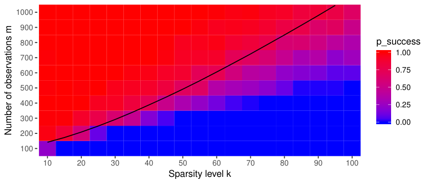
Next, we examine how the sample complexity of HWF scales with the signal sparsity $k$. The success rate vs signal sparsity $k$ and number of measurements $m$ is shown in Figure 4, which suggests that the sample complexity scales as $\mathcal{O}(k(x^{*}_{max})^{-2}\log\frac{n}{k})$, where we obtain $x^{*}_{max}$ as the average maximum coordinate of $100,000$ Gaussian $k$-sparse signals. We note that this scaling appears almost linear.

One of the parameters in Algorithm 1 is the number of restarts $\bar{b}$. Increasing $\bar{b}$ also increases the probability of HWF finding the true signal, but this comes at the cost of an increase in computational time. For the next experiment, we run HWF in the same setting as the first two experiments and vary the number of allowed restarts $\bar{b}$ from $1$ to $100$. Figure 5 shows that increasing the number of allowed restarts indeed increases the probability of successful reconstruction, where the success rate barely increases further as we increase the number of restarts $\bar{b}$ beyond $50$.

Next, we examine the convergence behavior of HWF. We also test HWF in the complex-valued setting, where we generate vectors $\mathbf{x}^{*},\mathbf{A}_{j}\sim\mathcal{N}(0,\frac{1}{2}\mathbf{I}_{1000})+i\mathcal{N}(0,\frac{1}{2}\mathbf{I}_{1000})$, set $990$ random entries of $\mathbf{x}^{*}$ to zero, normalize $\|\mathbf{x}^{*}\|_{2}=1$ and generate $m=500$ measurements $Y_{j}=|\mathbf{A}_{j}^{\mathrm{H}}\mathbf{x}^{*}|^{2}$. Figure 6 shows that HWF is also able to reconstruct complex signals. While HWF converges faster in the real case, both cases exhibit sublinear convergence after a short "warm-up" period. This can be explained by our parametrization. Consider the gradient $\nabla_{\mathbf{u}}F(\mathbf{U}^{t},\mathbf{V}^{t})=2\nabla F(\mathbf{X}^{t})\odot\mathbf{U}^{t}$: as the initialization size $\alpha$ is small, the gradient is small in the beginning due to the term $\mathbf{U}^{t}$. As $\mathbf{X}^{t}$ approaches $\mathbf{x}^{*}$, the term $\nabla F(\mathbf{X}^{t})$ converges to zero, which leads to linear convergence with a constant stepsize in the case of WF (Ma et al. 2018). With our parametrization, $\nabla_{\mathbf{u}}F$ (or $\nabla_{\mathbf{v}}F$) converges to zero faster than $\nabla_{\mathbf{x}}F$, as we typically have $U^{t}_{i}\rightarrow 0$ or $V^{t}_{i}\rightarrow 0$ (or both, if $x^{*}_{i}=0$), leading to sublinear convergence.

Finally, we present a numerical experiment that considers random initialization. In particular, we initialize $U^{0}_{i},V^{0}_{i}$ to small Gaussian noise $\mathcal{N}(0,0.01^{2})$ for all $i=1,\dots,n$. In general, we find that more samples are required for HWF to successfully reconstruct the signal $\mathbf{x}^{*}$ starting from a random initialization. Figure 7 shows that even in a setting with $n=1000$, $m=700$ and $k=10$, where HWF with random initialization does converge to the signal $\mathbf{x}^{*}$, the $\ell_{2}$ error $\operatorname{dist}(\mathbf{X}^{t},\mathbf{x}^{*})$ only decreases after an initial plateau, leading to slower convergence. This is in line with the intuition provided in the appendix, namely that $(i)$ the signal can still be recovered as coordinates on the support of $\mathbf{x}^{*}$ increase at a faster rate than coordinates not on the support, while $(ii)$ all coordinates only change at a very slow rate initially, because the inner product $(\mathbf{X}^{0})^{T}\mathbf{x}^{*}$ is closer to zero with random initialization compared to our proposed initialization (4), which leads to the initial plateau; see the appendix for more details.

In this paper, we proposed HWF, which is a simple algorithm for sparse phase retrieval. We proved that one step of HWF can be used as a support recovery tool, which, combined with existing algorithms such as SPARTA, yields a computationally fast algorithm with improved sample complexity, which reads $\mathcal{O}(k\log n)$ if the signal contains at least one large component and $k\geq\mathcal{O}(\log^{2}n)$. We have shown in numerical experiments that the sample complexity of HWF is lower than that of existing gradient based methods such as SPARTA and SWF, and comparable to PR-GAMP, which has been empirically shown to achieve linear sample complexity for Gaussian signals in some regimes (Schniter and Rangan 2015). While HWF does not require knowledge of the signal sparsity $k$, thresholding steps or any added regularization terms, this simplicity seems to come at the price of sublinear convergence and thus increased computational cost. We leave it to future work to investigate whether algorithmic principles such as the increasing step-size scheme considered in (Vaškevičius et al. 2019) or thresholding steps previously considered in the literature on sparse phase retrieval (e.g. (Cai et al. 2016; Wang et al. 2018; Zhang et al. 2018)) can be used to accelerate the convergence speed of HWF or to further improve its sample complexity beyond the level of the empirical results observed for PR-GAMP, which already relies on a combination of many such algorithmic principles (damping, normalization, EM steps). Compared to PR-GAMP, the simplicity of HWF makes the algorithm potentially more amenable to a rigorous theoretical investigation that can support the high-level analysis presented in our work.

References

- Arora et al. (2019) S. Arora, N. Cohen, W. Hu, and Y. Luo. Implicit regularization in deep matrix factorization. In Advances in Neural Information Processing Systems, pages 7411–7422, 2019.
- Balan et al. (2006) R. Balan, P. Casazza, and D. Edidin. On signal reconstruction without phase. Computational Harmonic Analysis, 20(3):345–356, 2006.
- Bayati and Montanari (2011) M. Bayati and A. Montanari. The dynamics of message passing on dense graphs, with applications to compressed sensing. IEEE Transactions on Information Theory, 57(2):764–785, 2011.
- Bunk et al. (2007) O. Bunk, A. Diaz, F. Pfeiffer, C. David, B. Schmitt, D. K. Satapathy, and J. F. Veen. Diffractive imaging for periodic samples: Retrieving one-dimensional concenctration profiles across microfluidic channels. Acta Crystallographica Section A: Foundations of Crystallography, 63(4):306–314, 2007.
- Cai et al. (2016) T. Cai, X. Li, and Z. Ma. Optimal rates of convergence for noisy sparse phase retrieval via thresholded Wirtinger flow. Annals of Statistics, 44(5):2221–2251, 2016.
- Candès and Li (2012) E. J. Candès and X. Li. Solving quadratic equations via PhaseLift when there are about as many equations as unknowns. Foundations of Computational Mathematics, 14(5):1017–1026, 2012.
- Candès et al. (2013) E. J. Candès, T. Strohmer, and V. Voroninski. PhaseLift: Exact and stable signal recovery from magnitude measurements via convex programming. Communications on Pure and Applied Mathematics, 66(8):1241–1274, 2013.
- Candès et al. (2015) E. J. Candès, X. Li, and M. Soltanolkotabi. Phase retrieval via Wirtinger flow: Theory and algorithms. IEEE Transactions on Information Theory, 61(4):1985–2007, 2015.
- Chen and Candès (2015) Y. Chen and E. J. Candès. Solving random quadratic systems of equations is nearly as easy as solving linear systems. In Advances in Neural Information Processing Systems, pages 739–747, 2015.
- Chen et al. (2019) Y. Chen, Y. Chi, J. Fan, and C. Ma. Gradient descent with random initialization: Fast global convergence for nonconvex phase retrieval. Mathematical Programming, 176(1–2):5–37, 2019.
- Chung and Lu (2006) F. Chung and L. Lu. Concentration inequalities and martingale inequalities: a survey. Internet Math., 3(1):79–127, 2006.
- Eldar and Mendelson (2014) Y. C. Eldar and S. Mendelson. Phase retrieval: Stability and recovery guarantees. Applied and Computational Harmonic Analysis, 36(3):473–494, 2014.
- Fienup (1982) J. R. Fienup. Phase retrieval algorithms: A comparison. Applied Optics, 21(15):2758–2769, 1982.
- Gerchberg and Saxton (1972) R. W. Gerchberg and W. O. Saxton. A practical algorithm for the determination of phase from image and diffraction. Optik, 35:237–246, 1972.
- Goldstein and Studer (2018) T. Goldstein and C. Studer. PhaseMax: Convex phase retrieval via basis pursuit. IEEE Transactions on Information Theory, 64(4):2675–2689, 2018.
- Gunasekar et al. (2017) S. Gunasekar, B. E. Woodworth, S. Bhojanapalli, B. Neyshabur, and N. Srebro. Implicit regularization in matrix factorization. In Advances in Neural Information Processing Systems, pages 6151–6159, 2017.
- Hand and Voroninski (2016) P. Hand and V. Voroninski. Compressed sensing from phaseless Gaussian measurements via linear programming in the natural parameter spaces. arXiv preprint arXiv:1611.05985, 2016.
- Hoff (2017) P. D. Hoff. Lasso, fractional norm and structured sparse estimation using a Hadamard product parametrization. Computational Statistics & Data Analysis, 115:186–198, 2017.
- Jaganathan et al. (2013) K. Jaganathan, S. Oymak, and B. Hassibi. Sparse phase retrieval: Convex algorithms and limitations. In Proceedings of IEEE International Symposium on Information Theory, pages 1022–1026, 2013.
- Jaganathan et al. (2016) K. Jaganathan, Y. C. Eldar, and B. Hassibi. Phase retrieval: An overview of recent developments. In A. Stern, editor, Optical Compressive Imaging, chapter 13, pages 263–296. Taylor Francis Group, Boca Raton, FL, 2016.
- Jagatap and Hedge (2017) G. Jagatap and C. Hedge. Fast, sample-efficient algorithms for structured phase retrieval. In Advances in Neural Information Processing Systems, pages 4917–4927, 2017.
- Jagatap and Hedge (2019) G. Jagatap and C. Hedge. Sample-efficient algorithms for recovering structured signals from magnitude-only measurements. IEEE Transactions on Information Theory, 65(7):4434–4456, 2019.
- Li and Voroninski (2013) X. Li and V. Voroninski. Sparse signal recovery from quadratic measurements via convex programming. SIAM Journal on Mathematical Analysis, 45(5):3019–3033, 2013.
- Li et al. (2018) Y. Li, T. Ma, and H. Zhang. Algorithmic regularization in over-parametrized matrix sensing and neural networks with quadratic activation. In Conference on Learning Theory, pages 2–47, 2018.
- Ma et al. (2018) C. Ma, K. Wang, Y. Chi, and Y. Chen. Implicit regularization in nonconvex statistical estimation: Gradient descent converges linearly for phase retrieval and matrix completion. In International Conference on Machine Learning, pages 3345–3354, 2018.
- Millane (1990) R. Millane. Phase retrieval in crystallography and optics. JOSA A, pages 394–411, 1990.
- Netrapalli et al. (2015) P. Netrapalli, P. Jain, and S. Sanghavi. Phase retrieval using alternating minimization. IEEE Transactions on Signal Processing, 63(18):4814–4826, 2015.
- Ohlsson et al. (2012) H. Ohlsson, A. Y. Yang, R. Dong, and S. S. Sastry. CPRL–an extension of compressive sensing to the phase retrieval problem. In Advances in Neural Information Processing Systems, pages 1367–1375, 2012.
- Qiu and Palomar (2017) T. Qiu and D. P. Palomar. Undersampled sparse phase retrieval via majorization–minimization. IEEE Transactions on Signal Processing, 65(22):5957–5969, 2017.
- Schechtman et al. (2014) Y. Schechtman, A. Beck, and Y. C. Eldar. GESPAR: Efficient phase retrieval of sparse signals. IEEE Transactions on Signal Processing, 62(4):928–938, 2014.
- Schniter and Rangan (2015) P. Schniter and S. Rangan. Compressive phase retrieval via generalized approximate message passing. IEEE Transactions on Signal Processing, 63(4):1043–1055, 2015.
- Sun et al. (2018) J. Sun, Q. Qu, and J. Wright. A geometric analysis of phase retrieval. Foundations of Computational Mathematics, 18(5):1131–1198, 2018.
- Vaškevičius et al. (2019) T. Vaškevičius, V. Kanade, and P. Rebeschini. Implicit regularization for optimal sparse recovery. In Advances in Neural Information Processing Systems, pages 2968–2979, 2019.
- Vershynin (2012) R. Vershynin. Introduction to the non-asymptotic analysis of random matrices. In Y. Eldar and G. Kutyniok, editors, Compressed Sensing, Theory and Applications, chapter 5, pages 210–268. Cambridge University Press, Cambridge, 2012.
- Voroninski and Xu (2016) V. Voroninski and Z. Xu. A strong restricted isometry property, with an application to phaseless compressed sensing. Applied and Computational Harmonic Analysis, 40(2):386–395, 2016.
- Waldspurger et al. (2015) I. Waldspurger, A. d’Aspremont, and S. Mallat. Phase recovery, MaxCut and complex semidefinite programming. Mathematical Programming, 149(1-2):47–81, 2015.
- Wang et al. (2017) G. Wang, G. B. Giannakis, and Y. C. Eldar. Solving systems of random quadratic equations via truncated amplitude flow. IEEE Transactions on Information Theory, 64(2):773–794, 2017.
- Wang et al. (2018) G. Wang, L. Zhang, G. B. Giannakis, M. Akçakaya, and J. Chen. Sparse phase retrieval via truncated amplitude flow. IEEE Transactions on Signal Processing, 66(2):479–491, 2018.
- Yang et al. (2013) Z. Yang, C. Zhang, and L. Xie. Robust compressive phase retrieval via L1 minimization with application to image reconstruction. arXiv preprint arXiv:1302.0081, 2013.
- Yuan et al. (2019) Z. Yuan, H. Wang, and Q. Wang. Phase retrieval via sparse Wirtinger flow. Journal of Computational and Applied Mathematics, 355:162–173, 2019.
- Zhang et al. (2017) H. Zhang, Y. Zhou, Y. Liang, and Y. Chi. A nonconvex approach for phase retrieval: Reshaped Wirtinger flow and incremental algorithms. Journal of Machine Learning Research, 18(141):1–35, 2017.
- Zhang et al. (2018) L. Zhang, G. Wang, G. B. Giannakis, and J. Chen. Compressive phase retrieval via reweighted amplitude flow. IEEE Transactions on Signal Processing, 66(19):5029–5040, 2018.
- Zhao et al. (2019) P. Zhao, Y. Yang, and Q.-C. He. Implicit regularization via Hadamard product over-parametrization in high-dimensional linear regression. arXiv preprint arXiv:1903.09367, 2019.
Appendix A Understanding the Dynamics of Hadamard Wirtinger Flow
As discussed in Section 3, the Hadamard parametrization has previously been applied to problems such as sparse recovery (Hoff 2017; Vaškevičius et al. 2019; Zhao et al. 2019) and matrix factorization (Gunasekar et al. 2017; Li et al. 2018; Arora et al. 2019), where it turns the additive updates of gradient descent into multiplicative updates. The combination of multiplicative updates and a small initialization was shown to lead to sparsity in the aforementioned problems, under the assumption of the restricted isometry property (RIP).
The problem of sparse phase retrieval that we consider is known to satisfy the RIP property, cf. (Voroninski and Xu 2016) for instance, and a similar explanation on why on-support variables and off-support variables can be made to grow at different speeds also holds in our setting. We now provide the main intuition behind the convergence properties of HWF by considering the evolution of the algorithm at the population level, i.e. in the case when . While a rigorous convergence investigation of HWF is outside the scope of the present work, the analysis that we now provide is instrumental to construct a good initialization for Algorithm 1.
Consider the simplified setting where is non-negative, i.e. for all . We can set in the parametrization, so that . Further, assume that we have access to the population risk (in other words, ), where is defined by . Its gradient can be computed as