Dynamical systems in perturbative scalar field cosmology

We consider a spatially flat RW background with a metric written as

where $a$ is the background scale factor, $H$ the Hubble variable, and $\gamma_{ij}$ is the flat spatial 3-metric, which in Cartesian coordinates is given by $\delta_{ij}$. The different time coordinates above are the clock time $t$, the conformal time $\eta$, and the $e$-fold time

where $N$ describes the number of background $e$-foldings with respect to some reference epoch at which $a=a_{0}$ and hence $N=0$.

The background equations that govern the matter distribution in a flat RW universe are the Friedman equation and the energy conservation equation

where overdot denotes derivative with respect to $t$.

The energy density $\rho$ and pressure $p$ for a minimally coupled scalar field $\varphi$ with a non-negative potential, $V=V(\varphi)$ are given by²² 2 See for example Liddle and Lyth (2000) [12], equations (3.3) and (3.4).

Making the obvious substitutions of equations (5) into (4) we obtain³³ 3 See for example Liddle and Lyth (2000) [12], equations (3.5) and (3.6).

where _,φ denotes $\frac{d}{d\varphi}$. Given a potential $V(\varphi)$ these equations determine $\varphi(t)$ and $H(t)$ when $\varphi$ and ${\dot{\varphi}}$ are specified at an initial time. The equation $\dot{a}=aH$ then determines the scale factor $a$ as a quadrature.

Before continuing we digress to introduce the deceleration parameter $q$ which is useful in describing the dynamics:

It follows from (4) and (5) that

We find it convenient to use the $e$-fold time $N$ instead of the clock time $t$ as our starting point and to introduce the following quantities:⁴⁴ 4 The factors of $\sqrt{6}$ are included in the definitions (9) in order to simplify future algebra. The reason for using the notation $\Sigma$ for the kernel is because this variable plays a similar role as Hubble-normalized shear, which is typically denoted with the kernel $\Sigma$, see e.g. [13].

where a ^′ denotes the $e$-fold time derivative $\frac{d}{dN}=H^{-1}\frac{d}{dt}$. Equations (7) and (8) assume the form

The definitions (9) have the effect of eliminating the explicit appearance of $H$ in the governing equations (6). The second equation becomes

while the second order ODE is replaced by two coupled first order ODEs:⁵⁵ 5 As a first step divide both equations by $H^{2}$ and note that $$\frac{d}{dt}=H\frac{d}{dN},\quad\frac{d^{2}}{dt^{2}}=H^{2}\left(\frac{d^{2}}{dN^{2}}-(1+q)\frac{d}{dN}\right).$$ Use (10) to eliminate $1+q$, and use the definition of $\lambda$ in (9) and (11) to eliminate $V_{,\varphi}$ in (6).

In general the scalar $\lambda$, defined by (9), is a function of $\varphi$ but in the case of an exponential potential $\lambda$ is constant. We use this constant value to define $V$ according to⁶⁶ 6 This labelling of $V$ is consistent with the definition (9) of $\lambda$.

Since $\lambda$ is now a constant (12a) decouples from (12b), and can be used to determine $\varphi$ by quadrature once (12b) has been solved. Thus (12b) contains the essential dynamical information for the background scalar field in the case of an exponential potential. Since $V$ has been defined to be positive, it follows from (9) that $\Omega_{V}$ is positive and hence from (11) that $\Sigma_{\varphi}$ is bounded: $-1<\Sigma_{\varphi}<1$. However, since the right hand side of (12b) is continuously differentiable and zero when $\Sigma_{\varphi}=\pm 1$ it is possible and desirable to extend the range of $\Sigma_{\varphi}$ to include the invariant boundary values $\Sigma_{\varphi}=\pm 1$:

Equation (10) now restricts the deceleration parameter:

where $q=-1$ if $\Sigma_{\varphi}=0$ and $q=2$ if $\Sigma_{\varphi}=\pm 1$.

To describe the linear perturbations of the scalar field we use the perturbed KG equation, which has a particularly simple form if one uses as dependent variable the linear perturbation of the scalar field in the uniform (flat) curvature gauge,⁷⁷ 7 Once one chooses the uniform curvature gauge or the comoving gauge as we do in section 6, there is no remaining gauge freedom. See for example [14] or [15] section 3. which we denote by $\varphi_{\mathrm{c}}$. An advantage of using the uniform curvature gauge is that the metric perturbations can be eliminated from the KG equation using the Einstein equations, leaving a closed equation which can be written as follows (see, e.g., Uggla and Wainwright (2019) [16], section 3, Appendix A.3 and in particular equation (A.21)):

where $\varphi$ is the background scalar field,

and ${\bf D}^{2}$ is the background spatial Laplacian associated with $\gamma_{ij}$. For an exponential potential (13) the KG equation assumes the form

in the notation of (9).

The state space ${\cal S}={\cal B}\times{\cal P}$ is a three-dimensional product space where ${\cal B}$ is the background state space, with coordinates $\Sigma_{\varphi}$ and ${\bar{Z}}$, subject to

while ${\cal P}$ is the perturbation state space, which is a circle parameterized by the angular coordinate $\theta$ of period $2\pi$. We can visualize ${\cal S}$ by rotating the rectangle (37) through $2\pi$ radians about a line $\Sigma_{\varphi}=b<-1$ to form a solid finite cylinder with a cylindrical hole along its axis. The surfaces of constant $\Sigma_{\varphi}$ are coaxial cylinders whose common axis defines the $\bar{Z}$-axis with $0\leq\bar{Z}\leq 1$. The cylinders $\Sigma_{\varphi}=1$ and $\Sigma_{\varphi}=-1$ form the outer and inner boundaries of the solid cylinder, respectively, and are invariant sets of the dynamical system, as follows from equation (34a). The planes ${\bar{Z}}=0$ and ${\bar{Z}}=1$ form the bottom and top of the solid cylinder, respectively, and are also invariant sets as follows from equation (34b). In this representation the state space ${\cal B}\times{\cal P}$ is a compact subset of ${\mathbb{R}}^{3}$. On the other hand if we use the perturbation variable $y=\tan\theta$ then the state space ${\cal B}\times{\cal P}$ is the infinite slab in ${\mathbb{R}}^{3}$ defined by the inequalities (35).¹³¹³ 13 Since $\tan(\theta+\pi)=\tan\theta$, the mapping $y=\tan\theta$ is two-to-one and therefore when $\theta$ makes one revolution ($0\rightarrow 2\pi$) $y$ has to be traversed twice $-\infty\rightarrow+\infty$.

The invariant sets $\Sigma_{\varphi}=1$ and $\Sigma_{\varphi}=-1$ describe the limiting case of a massless scalar field model ($V=0$, see equations (9) and (12)). We will therefore refer to the invariant sets $\Sigma_{\varphi}=\pm 1$ as the two components of the massless scalar field boundary. Because of the physical interpretation of ${\bar{Z}}$ (see section 3) we refer to the invariant set ${\bar{Z}}=0$ as the long wavelength boundary, and ${\bar{Z}}=1$ as the short wavelength boundary. In addition to the above invariant boundary sets there is an important invariant set given by the interior cylinder with $\Sigma_{\varphi}=\lambda$.

We obtain the fixed points of the dynamical system by equating the right hand sides of (34) to zero. It follows that if $0\leq\lambda<1$ and $\lambda\neq 1/\sqrt{3}$ then all the fixed points of the dynamical system lie in the long and short wavelength boundary sets $\bar{Z}=0$ and $\bar{Z}=1$. On the $\bar{Z}=0$ boundary they either satisfy $\Sigma_{\varphi}=\lambda$ or $\Sigma_{\varphi}^{2}=1$. There are two hyperbolic fixed points with $\Sigma_{\varphi}=\lambda$ which we denote by $\mathrm{A}_{\lambda}$ and $\mathrm{S}_{\lambda}$:

There are also two non-hyperbolic fixed points denoted by $\mathrm{M}_{\pm}$, given by

However, when we draw pictures of the global state space we will use $\theta$ as the perturbation variable, with $\tan\theta=y$. Then $y=0$ corresponds to $\theta=n\pi,n=0,1$, where $y=-3(1-\lambda^{2})$ corresponds to $\theta=\chi+n\pi,n=0,1$, where $\chi=-\arctan 3(1-\lambda^{2}).$ In other words, each of the fixed points (38) and (39) appear twice as $\theta$ makes one revolution ($0\rightarrow 2\pi$).

The short wavelength boundary ${\bar{Z}}=1$ also plays an important role. On ${\bar{Z}}=1,$ using $\theta$ as the perturbation variable, the differential equations (34) and (36) simplify to

There are therefore two lines of (non-hyperbolic) fixed points at ${\bar{Z}}=1$ with constant $\Sigma_{\varphi}$ given by $\cos\theta=0$, i.e., $\theta=\pi/2+n\pi,n=0,1$. Except at these fixed points, $\theta$ is monotonically decreasing on ${\bar{Z}}=1$ at constant $\Sigma_{\varphi}$. It follows that the invariant set ${\bar{Z}}=1$ is spanned by a family of heteroclinic cycles (concentric circles) given by $\Sigma_{\varphi}=\mathrm{const}.$, with $-1\leq\Sigma_{\varphi}\leq 1$. At $\theta=\pi/2+n\pi$ equation (36) takes the form

which implies that orbits in the vicinity of $\bar{Z}=1$ shadow the heteroclinic cycles and do not end at the fixed points on these cycles. Moreover, as we will see, asymptotics are associated with $\Sigma_{\varphi}=\lambda,\pm 1$, and hence it is only the heteroclinic cycles at these values of $\Sigma_{\varphi}$ which are of asymptotic relevance. We will denote these heteroclinic cycles by ${\cal H}_{\lambda}$, ${\cal H}_{\pm 1}$, respectively (this use of $\cal H$ with subscripts should not be confused with ${\cal H}=aH$).

In Fig. 1 we show the key invariant sets and fixed points in the state space ${\cal S}={\cal B}\times{\cal P}$.

The background state space $\cal B$ with coordinates $(\Sigma_{\varphi},{\bar{Z}})$ is defined by the inequalities

The differential equations that define a dynamical system on ${\cal B}$ are the first two equations of the system (34). In the background it is convenient to use the usual $e$-fold time $N$ instead of the modified time ${\bar{N}}$, leading to the following equations:

The fixed points of this dynamical system can be found by inspection. If $\lambda\neq 1/\sqrt{3}$ there are six isolated fixed points, which lie on the boundary of the rectangle (42):

The fixed points ${\bar{Z}}=0,\,\Sigma_{\varphi}=\pm 1$ are local sources and form the past attractor, while the fixed points ${\bar{Z}}=1,\Sigma_{\varphi}=\pm 1$ are saddles for all values of $\lambda$.

The future attractor depends on the value of the parameter $\lambda$, and is given by the following two fixed points:

The line $\Sigma_{\varphi}=\lambda\neq 1/\sqrt{3}$ is a special orbit joining the fixed points i) and ii). If $\lambda=1/\sqrt{3}$ (and therefore $q=0$) this line becomes a line of fixed points, which corresponds to a bifurcation that transfers stability from i) to ii) as $\lambda$ increases.

The qualitative behaviour of typical and special orbits in the two cases $0\leq\lambda<1/\sqrt{3}$ and $1/\sqrt{3}<\lambda<1$ is illustrated in Fig. 2.

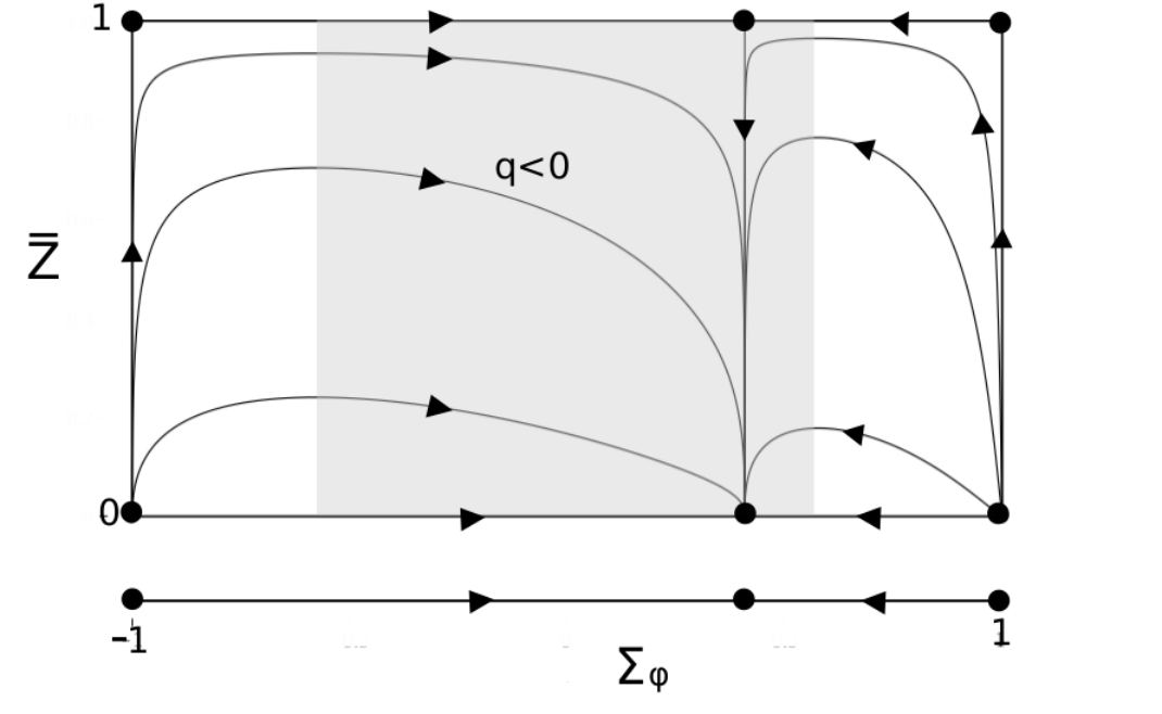
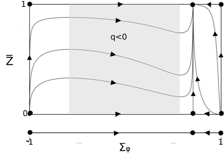
Referring to Fig. 2 we can summarize the asymptotic behaviour of the orbits in the background state space $\cal B$ for $\lambda\neq 1/\sqrt{3}$ as follows. For evolution into the future for all orbits with $\Sigma_{\varphi}^{2}<1$ we have

Into the past all orbits with $\Sigma_{\varphi}\neq\lambda$ satisfy,

while the special case $\Sigma_{\varphi}=\lambda$ results in

For the special case $\Sigma_{\varphi}=\pm 1$ we have

In the next section we will use these results to determine the asymptotic behaviour of the orbits in the full state space ${\cal B}\times{\cal P}$.

Before continuing we make some remarks relating our description of the background dynamics to previous research. The first paper to give a dynamical systems analysis of a scalar field with exponential potential is Halliwell (1987) [17], who used the background scalar field $\varphi$ and an exponential representation of the cosmological scale factor as variables.¹⁴¹⁴ 14 In his figure 2, the flat background case is represented by the bold face hyperbola, and this corresponds to our background state space on the $\Sigma_{\varphi}$-axis shown in our Figure 2 since the exponential scale factor variable decouples in the flat case. The fixed point A in his figure 2 is the future attractor, which corresponds to our fixed point with $\Sigma_{\varphi}=\lambda$. From our perspective, the limitation of his approach is that the state space is unbounded. The bounded variable $\Sigma_{\varphi}$ that we are using is not new. It has been introduced before in the context of a scalar field with an exponential potential by Coley et al (1997) [18] and by Copeland et al (1998) [19]. Both these references considered more general background problems than the present one: Coley et al studied anisotropic Bianchi models and Copeland et al added a perfect fluid with a linear equation of state to the scalar field. The variable $d\varphi/dN$, which is proportional to $\Sigma_{\varphi}$, is now commonly used to describe scalar fields in cosmology.¹⁵¹⁵ 15 See for example, Urena-Lopez (2012) [20], equation (2.3), Tsujikawa (2013) [21], equation (16) and Alho and Uggla (2015) [22], equation (8).

Our state space ${\cal B}$ differs in an important way from [17, 19], in that it also describes the dynamics of the variable $Z=k^{2}/{\cal H}^{2}$, compactified to give ${\bar{Z}}$, whose evolution is determined by $\Sigma_{\varphi}$ through the differential equation (43b), which leads to the two dimensional state space in our figure 2. This yields a complete description of the dynamics of a scalar field with exponential potential in a flat FL background needed to determine the evolution of perturbations on this background, which is the main goal of this paper. This representation of the dynamics, which to the best of our knowledge is new, has several advantages. It shows directly in which regions of the state space there is accelerated expansion (the shaded regions in figure 2, in which $q=3\Sigma_{\varphi}^{2}-1<0$ and where thereby $Z$ and $\bar{Z}$ are monotonically decreasing), and highlights the physical interpretation of the parameter $\lambda$ in the potential. Referring to our figure 2, if $\lambda<1/\sqrt{3}$ then all orbits eventually enter and remain in the region of accelerated expansion and thus the orbits describe universes that undergo future accelerated expansion. On the other hand if $\lambda<1/\sqrt{3}$ orbits that are past asymptotic to $\Sigma_{\varphi}=1$ do not enter the shaded region and hence never undergo accelerated expansion, while orbits that are past asymptotic to $\Sigma_{\varphi}=-1$ enter and then leave the shaded region and hence undergo transient accelerated expansion. We note that the general orbits in Figure 2 have been given explicitly in parametric form $H(u),\varphi(u),$ where $u$ is a parameter, by Salopek and Bond (1990) [23], and analyzed qualitatively (see equations (3.2) and their figure 1). Our state space picture shows this behaviour directly.

Since the full state space has a product structure ${\cal S}={\cal B}\times{\cal P}$, the limits of $\Sigma_{\varphi}$ and $\bar{Z}$ as $N\rightarrow\pm\infty$ given by equations (46), (47), (48) and (49), which we derived in the background state space ${\cal B}$ (see also Fig. 2), are also valid in ${\cal B}\times{\cal P}$, and we can use these results to determine the asymptotic behaviour of the orbits in the full state space. We still limit the discussion to $0\leq\lambda<1$, and we also exclude the bifurcation value $\lambda=1/\sqrt{3}$. The restrictions imposed in deriving (46) and (47) require that we consider separately the generic orbits and the special orbits that satisfy $\Sigma_{\varphi}=\lambda$ and $\Sigma_{\varphi}=\pm 1$ with constant deceleration parameter $q$. We refer to the case $\Sigma_{\varphi}=\lambda$ as the (interior) scale-invariant orbits,¹⁶¹⁶ 16 The solutions corresponding to orbits with $\Sigma_{\varphi}=\lambda>0$ are invariant under constant conformal scalings and admit a homothetic Killing vector field. The orbits with $\Sigma_{\varphi}=\lambda=0$ correspond to the one-parameter family of de Sitter solutions, where a constant scaling scales the dimensional cosmological constant that is parametrizing the family of solutions. Constant conformal scalings thereby result in the same solution when $\lambda>0$ while they lead to a new member in the same family of solutions when $\lambda=0$. The close connection between the two classes is illustrated by that both $\lambda>0$ and $\lambda=0$ yield constant values for dimensionless scalars such as $\Sigma_{\varphi}$ and $q$. For simplicity we will therefore also refer to $\lambda=0$ as belonging to the scale-invariant case. and the orbits with $\Sigma_{\varphi}=\pm 1$ as the massless scalar field orbits (although they also correspond to scale-invariant solutions). On recalling that $q=3\Sigma_{\varphi}^{2}-1$, we have

First as regards the generic orbits it follows from equations (46) and (47) that

• Gi)

  all generic orbits are past asymptotic to one of the fixed points $\mathrm{M}_{\pm}$, which form the past attractor of the dynamical system,

• Gii)

  if $\lambda<1/\sqrt{3}$ then a two parameter family of orbits is future asymptotic to the fixed point $\mathrm{A}_{\lambda}$, which forms the future attractor; in addition a one-parameter family of orbits is future asymptotic to the fixed point $\mathrm{S}_{\lambda}$,

• Giii)

  if $\lambda>1/\sqrt{3}$ then all orbits are future asymptotic to the heteroclinic cycle ${\cal H}_{\lambda}$, which forms the future attractor.

We give some details of the derivation of the result Gii) at the end of this section.

We now describe the acceleration/deceleration properties of these generic models.¹⁷¹⁷ 17 The region of state space in which there is accelerated expansion is a cylindrical shell in the state space ${\cal S}={\cal B}\times{\cal P}$, given by the inequalities $-1/\sqrt{3}<\Sigma_{\varphi}<1/\sqrt{3}.$ This region can be visualized by rotating the shaded region in figure 2 about a line $\Sigma_{\varphi}=b<-1,$ as described at the beginning of section 4.1. Since $q=3\Sigma_{\varphi}^{2}-1$ we can draw the following conclusions by referring to Fig. 2 and using the results Gi)-Giii) above:

• i)

  If $\lambda<1/\sqrt{3}$, then all models undergo future acceleration,

• ii)

  If $\lambda>1/\sqrt{3}$ then all models undergo future deceleration. However, there are two subcases. Orbits that are past asymptotic to $\mathrm{M}_{-}$ yield models that undergo transient acceleration, i.e. they have a finite epoch during which $q<0$, see Fig. 2; orbits that are past asymptotic to $\mathrm{M}_{+}$ yield models that are forever decelerating, i.e. $q>0$ at all times.

Fig. 3 shows examples of generic orbits in the two cases $0\leq\lambda<1/\sqrt{3}$ and $1/\sqrt{3}<\lambda<1$.

Before continuing we make a remark concerning the physical interpretation of Figure 3. It is helpful to think how the orbits are generated numerically. One chooses initial values for $\Sigma_{\varphi},{\bar{Z}}$ and $\theta$ and then integrates numerically forwards and backwards to generate an orbit.¹⁸¹⁸ 18 The usual way to numerically integrate the perturbation equations for scalar fields is to first integrate the background equations, and then use the output to integrate the perturbed Klein-Gordon equation to determine the real and imaginary parts of the Fourier transform of the scalar field perturbation, for a given wave number $k$. One is thereby treating the perturbed Klein-Gordon equation as a non-autonomous differential equation, in contrast to our dynamical systems approach. See for example Huston and Malik (2009) [24] (this paper also covers second order perturbations) and Martin and Ringeval (2006) [25] (see section 4.1). One can use the initial value of ${\bar{Z}}$ in conjunction with equation (31) to determine the wave number $k$ in terms of the value of the Hubble scalar $H_{0}$ at the initial time $a_{0}=1,N_{0}=0$:

In this way one can generate a family of orbits corresponding to different wave numbers.

Next, as regards the interior scale-invariant orbits ($\Sigma_{\varphi}=\lambda<1$) it follows from equation (48) that

• Ai)

  if $0\leq\lambda<1/\sqrt{3}$ (i.e. $q<0$) then a scale-invariant orbit is past asymptotic to the heteroclinic cycle ${\cal H}_{\lambda}$ and is future asymptotic to the fixed point $\mathrm{A}_{\lambda}$, apart from one exceptional orbit that is future asymptotic to the fixed point $\mathrm{S}_{\lambda}$,

• Aii)

  if $1/\sqrt{3}<\lambda<1$ (i.e. $q>0$) then a scale-invariant orbit is future asymptotic to the heteroclinic cycle ${\cal H}_{\lambda}$ and is past asymptotic to the fixed point $\mathrm{S}_{\lambda}$, apart from one exceptional orbit that is past asymptotic to the fixed point $\mathrm{A}_{\lambda}$.

Representative scale-invariant orbits are depicted in Fig. 4 (recall that there are two copies of fixed points and orbits when using $\theta$ instead of $y$, related to each other by $\theta\rightarrow\theta+\pi$).

Finally, as regards the massless scalar field orbits ($\Sigma_{\varphi}=\pm 1$) it follows from equations (49) that such an orbit is past asymptotic to one of the fixed points $\mathrm{M}_{\pm}$, and is future asymptotic to one of the heteroclinic cycles ${\cal H}_{\pm 1}$. Representative massless scalar field orbits are depicted in Fig. 5.

In deriving the result Gii), the limits (46) in ${\cal B}$ imply that $\lim_{N\rightarrow\infty}\Sigma_{\varphi}=\lambda,$ and $\lim_{N\rightarrow\infty}{\bar{Z}}=0$ in the state space ${\cal S}={\cal B}\times{\cal P}$. It follows that the orbits in question are future asymptotic to the one dimensional invariant set $\Sigma_{\varphi}=\lambda,\bar{Z}=0$ (a circle). Since this circle contains the two hyperbolic fixed points $\mathrm{A}_{\lambda}$ and $\mathrm{S}_{\lambda}$, the orbits in question must be future asymptotic to one of these fixed points. The final step is to note that in this case $\mathrm{A}_{\lambda}$ is a sink and $\mathrm{S}_{\lambda}$ is a saddle with a two dimensional stable manifold.

The local stability properties of $\mathrm{A}_{\lambda}$ and $\mathrm{S}_{\lambda}$ also yield the local stability properties for Ai) and Aii): in Ai) $\mathrm{A}_{\lambda}$ is a sink and $\mathrm{S}_{\lambda}$ is a saddle on the interior scale-invariant set $\Sigma_{\varphi}=\lambda$, while in Aii) $\mathrm{S}_{\lambda}$ is a source and $\mathrm{A}_{\lambda}$ is a saddle, see Fig. 4.

In this subsection we will give asymptotic expansions for $\Sigma_{\varphi}$, $Z$, $y$ and $\varphi_{\mathrm{c}}$ in terms of the $e$-fold time $N$ in the vicinity of the fixed points in the long wavelength boundary set $Z=0$. When it comes to $\varphi_{\mathrm{c}}$, we will focus on the future accelerating case $0\leq\lambda<1/\sqrt{3}$, for which we need $\varphi_{\mathrm{c}}$ in section 6.

References

- [1] A. Alho, C. Uggla, and J. Wainwright. Perturbations of the lambda-cdm model in a dynamical systems perspective. JCAP, 09:045, 2019.
- [2] D. H. Lyth and E. D. Stewart. The curvature perturbation in power law (e.g extended) inflation. Phys. Lett. B, 274:168, 1992.
- [3] R. Durrer. The cosmic microwave background. Cambridge University Press, 2008.
- [4] S. Weinberg. Cosmology. Oxford university press, 2008.
- [5] A. E. Romano, S. Mooij, and M. Sasaki. Adiabaticity and gravity theory independent conservation laws for cosmological perturbations. Phys. Lett. B, 755:464, 2016.
- [6] S. Mooij and G. A. Palma. Consistently violating the non-gaussian consistency relation. Journal of Cosmology and Astroparticle Physics, 11:025, 2015.
- [7] N. C. Tsamis and R. P. Woodard. Improved estimates of cosmological perturbations. Phys. Rev. D, 69:084005, 2004.
- [8] W. H. Kinney. Horizon crossing and inflation with large . Phys. Rev. D, 72:023515, 2005.
- [9] M. H. Namjoo, H. Firouzjahi, and M. Sasaki. Violation of non-gaussianity consistency relation in a single-field inflationary model. EPL (Europhysics Letters), 101:39001, 2013i.
- [10] X. Chen, H. Firouzjahi, M. H. Namjoo, and M. Sasaki. A single field inflation model withlarge local non-gaussianity. Europhys. Lett., 102(59001), 2013.
- [11] J. Martin, H. Motohashi, and T. Suyama. Ultra slow-roll inflation and the non-gaussianity consistency relation. Phys. Rev. D, 87:023514, 2013.
- [12] A. R. Liddle and D. H. Lyth. Cosmological inflation and large-scale structure. Cambridge University Press, 2000.
- [13] J. Wainwright and G. F. R. Ellis. Dynamical systems in cosmology. Cambridge University Press, 1997.
- [14] K. A. Malik and D. Wands. Cosmological perturbations. Physics Reports, 475:1–51, 2009.
- [15] C. Uggla and J. Wainwright. Second order cosmological perturbations: simplified gauge change formulas. Class. Quantum Grav., 36:035004, 2019.
- [16] C. Uggla and J. Wainwright. The general solution at large scale for second order perturbations in a scalar field dominated universe. Journal of Cosmology and Astroparticle Physics, 2019(06):021–021, 2019.
- [17] J. Halliwell. Scalar fields in cosmology with an exponential potential. Phys. Lett. B, 185:341, 1987.
- [18] A. A. Coley, J. Ibánez, and R. J. van den Hoogen. Homogeneous scalar field cosmologies with an exponential potential. Journal of Mathematical Physics, 38:17, 1997.
- [19] E. J. Copeland, A. R. Liddle, and D. Wands. Exponential potentials and cosmological scaling solutions. Phys. Rev. D, 57:4686, 1998.
- [20] L. A. Urena-Lopez. Unified description of the dynamics of quintessential scalar fields. JCAP, 2012:035, 2012.
- [21] S. Tsujikawa. Quintessence: a review. Class. Quantum Grav., 30:214003, 2013.
- [22] A. Alho and C. Uggla. Scalar field deformations of lambda-cdm cosmology. Phys. Rev. D, 92(10):103502, 2015.
- [23] D. S. Salopek and J.R. Bond. Nonlinear evolution of long-wavelength metric fluctuations in inflationary models. Phys. Rev. D, 42:3936, 1990.
- [24] I. Huston and K. A. Malik. Numerical calculation of second order perturbations. JCAP, 09:019, 2009.
- [25] J. Martin and C.Ringeval. Inflation after wmap3: confronting the slow-roll and exact power spectra with cmb data. JCAP, 08:009, 2006.
- [26] C. Uggla and J. Wainwright. Second-order cosmological perturbations: New conserved quantities and the general solution at super-horizon scale. Phys. Rev. D, 100:023544, 2019.
- [27] C. Uggla and J. Wainwright. Second order cosmological perturbations: dynamics. Phys. Rev. D, 98:103534, 2018.
- [28] C. Uggla. Asymptotic cosmological solutions: orthogonal bianchi type-ii models. Class. Quantum Grav., 6(3):383, 1989.
- [29] A. Alho, J. Hell, and C. Uggla. Global dynamics and asymptotics for monomial scalar field potentials and perfect fluids. Class. Quant. Grav., 32(14):145005, 2015.
- [30] A. Alho and C. Uggla. Global dynamics and inflationary center manifold and slow-roll approximants. Journal of Mathematical Physics, 56(012502), 2015.
- [31] A. Alho and C. Uggla. Inflationary -attractor cosmology: A global dynamical systems perspective. Phys. Rev. D, 95(8):083517, 2017.
- [32] K. Dimopoulos and C. Owen. Quintessential inflation with -attractors. J. of Cosmology and Astroparticle Physics, 06:027, 2017.
- [33] P. J. E. Peebles and A. Vilenkin. Quintessential inflation. Phys. Rev. D, 59:063505, 1999.