跳到论文正文
W Papers独立论文阅读器 arXiv:2006.00636 论文正文 计算阅读时间 · 0%
引用这篇论文根据当前论文元数据生成,正式投稿前建议核对。


License: arXiv.org perpetual non-exclusive license
arXiv:2006.00636v2 [math.ST] 15 Dec 2020

Sequential change point detection in high dimensional time series

Josua Gösmann, Christina Stoehr, Johannes Heiny and Holger Dette Affiliation: Ruhr-Universität Bochum Affiliation: Fakultät für Mathematik Affiliation: 44780 Bochum, Germany
Abstract

Change point detection in high dimensional data has found considerable interest in recent years. Most of the literature either designs methodology for a retrospective analysis, where the whole sample is already available when the statistical inference begins, or considers online detection schemes controlling the average time until a false alarm. This paper takes a different point of view and develops monitoring schemes for the online scenario, where high dimensional data arrives successively and the goal is to detect changes as fast as possible controlling at the same time the probability of a type I error of a false alarm. We develop a sequential procedure capable of detecting changes in the mean vector of a successively observed high dimensional time series with spatial and temporal dependence. The statistical properties of the method are analyzed in the case where both, the sample size and dimension tend to infinity. In this scenario, it is shown that the new monitoring scheme has asymptotic level alpha under the null hypothesis of no change and is consistent under the alternative of a change in at least one component of the high dimensional mean vector. The approach is based on a new type of monitoring scheme for one-dimensional data which turns out to be often more powerful than the usually used CUSUM and Page-CUSUM methods, and the component-wise statistics are aggregated by the maximum statistic. For the analysis of the asymptotic properties of our monitoring scheme we prove that the range of a Brownian motion on a given interval is in the domain of attraction of the Gumbel distribution, which is a result of independent interest in extreme value theory. The finite sample properties of the new methodology are illustrated by means of a simulation study and in the analysis of a data example.

Keywords and phrases: high dimensional time series, change point analysis, sequential monitoring, Gaussian approximation, bootstrap

AMS Subject classification: Primary 62M10, 62H15; Secondary 62G20; 60G70

1 Introduction

As digital transformation processes have accelerated during the last decades, new technologies like smartphones or car sensors are able to gather large amounts of data. Due to this development companies, states, research institutes etc. face the problem to manage, monitor and examine huge data sets, which regularly exceed the means of traditional tools. Thus the demand for so-called big data technology is steadily growing and thereby the requirement for theoretical foundation has put a lot of attention at the topic of high dimensional statistics in recent years.

Especially, the topic of change point analysis or detection of structural breaks has regained attraction and numerous authors have started to embed commonly used multivariate methods into a high dimensional framework or even develop new methodology from scratch. Among many others, high dimensional change point problems have been considered by Cho and Fryzlewicz, 2015, Wang and Samworth, 2018a, who develop methodology to identify multiple change points by a (wild) binary segmentation algorithm under sparsity assumptions. Jirak, 2015b and Dette and Gösmann, 2018 aggregate component-wise CUSUM-statistics by the maximum functional to detect structural breaks in a sequence of means of a high dimensional time series. Lévy-Leduc and Roueff, 2009 analyze internet traffic data, by applying a compenent-wise CUSUM-test to dimension-reduced censored data.

Enikeeva and Harchaoui, 2019 employ the Euclidean norm of the CUSUM-process to obtain a linear and a scan statistic of χ2\chi^{2}-type, that is minimax-optimal under the regime of independent Gaussian observations. Change point problems in high dimensional covariance matrices are studied by Wang et al., 2017, Avanesov and Buzun, 2018 and Dette et al., 2018 using (wild) binary segmentation, multiscale methods and U-statistics, respectively. U-statistics are also used by Wang et al., 2019 and Wang and Shao, 2020 to develop testing and estimation methodology for a structural break in the mean.

All listed references on high dimensional change point problems have in common that the proposed methods are designed for a retrospective or offline analysis, where the whole sample is already available when the statistical inference is commenced. In contrast to this, sequential change point detection deals with methods that are applicable for monitoring data in a so-called online scenario. In such a setup, data arrives steadily and methods are constructed to detect changes as fast as possible, while the problem is reevaluated with each new data point. Starting with the seminal paper of Wald, 1945 on the sequential probability ratio test, an enormous amount of literature has been published discussing the problem from different perspectives. Several concepts have been proposed to model the situation of online monitoring and we discuss the different paradigms addressing the sequential change point problem in more detail at the end of this introduction.

To the authors best knowledge, a common feature of most of the literature on sequential change point detection consists in the fact that it does not consider the time and spatially dependent high dimensional scenario, where the dimension of the data increases with the sample size. The purpose of the present paper is to address this problem in the context of detecting changes in the mean. For this purpose, we follow consider the paradigm of Chu et al., 1996, which provides a model for online change point detection, such that the probability of a type I error (false alarm) can be controlled (asymptotically). We develop a sequential algorithm in the high dimensional regime aggregating component-wise sequential detection schemes by the maximum statistic. For the individual components we use a novel monitoring procedure, which screens for all possible positions of the change point and takes into account that the change does not necessarily occur in the first observations after the initial sample - see Section 2 for more details. A nice feature of this approach consists in the fact that the limiting distribution of the statistic used to monitor each component (after appropriate standardization) is given by the range of the Brownian motion, that is 𝕄=max0≤t≤q⁡W⁡(t)−min0≤t≤q⁡W⁡(t)\mathbb{M}=\max_{0\leq t\leq q}W(t)-\min_{0\leq t\leq q}W(t), where WW is a Brownian motion on the interval [0,q][0,q] and 0<q<10<q<1 is a known constant. The distribution of the random variable 𝕄\mathbb{M} appears as the weak limit of the range of cumulative sums of i.i.d. random variables with variance 11 [see Feller, 1951], and we will show that it belongs to the domain of attraction of the Gumbel distribution. This result is of independent interest in extreme value theory and allows us to aggregate component-wise statistics by the maximum.

As a consequence we can develop a sequential monitoring scheme in the high dimensional regime using the quantiles of the Gumbel distribution. For this purpose, we combine Gaussian approximations tools for high dimensional statistics [see Chernozhukov et al., 2013; Zhang and Cheng, 2018] and show that the statistic can be approximated by a counterpart computed from Gaussian observations with the same long-run correlation structure as the observed time series. Using Gaussian comparison and anti-concentration inequalities we show that this statistic is sufficiently close to the maximum of ranges of dependent Brownian motions. Finally, we use Poisson approximation via the Chen-Stein method to eliminate the independence condition, such that the new result for the independent case can be applied. As the rates of most convergence results in extreme value theory are known to be rather slow, we also propose a simple bootstrap procedure, which improves the performance of the sequential monitoring scheme for sample sample sizes. To our best knowledge, our paper provides the first rigorous analysis of a sequential change point detector in the high dimensional regime for the model introduced by Chu et al., 1996.

The remaining part of this paper is organized as follows. We conclude this introduction with a discussion and comparison of the different philosophies in sequential change point detection. In Section 2, we introduce the specific testing problem under consideration and present the new monitoring procedure for structural breaks in the sequence of means from a high dimensional time series. Section 3 is devoted to our main results and to the analysis of the asymptotic properties of the new procedure. In particular, we prove that the maximum of the individual test statistics converges weakly (with increasing dimension and initial sample size) to a Gumbel distribution. These results are used to show that the monitoring scheme has asymptotic level α\alpha and is consistent. In Section 4, we investigate the finite sample properties of the new procedures by means of a simulation study and illustrate potential applications in a data example. Finally, all proofs are deferred to Appendix B in the online supplement.

Related literature - two paradigms in sequential change point detection

In the remaining part of this section, we briefly discuss to ways of modelling the problem of sequential change point detection, which have developed rather independently in the last 2525 years. The list of references cited below is by no means complete, because both modelling approaches have been used intensively in the literature. Rather it represents a selective choice of the authors with the goal to put the approach proposed in this paper in the appropriate context. Sequential change point detection in the high dimensional scenario, where the dimension increases with the sample size, has barely been studied in the liteature, where some of the relevant exceptions are cited below.

The different models in the literature are used to address different criteria for quantifying the propensity of a detection scheme to cause false alarms. The traditional Statistical Process Control (SPC)-approach has its focus on a fast change point detection, where the average time from monitoring start to a false alarms is controlled.

On the other hand, if the costs of a false alarm are heavy, for instance if a large portfolio has to be restructured in portfolio management, it might be more reasonable to control the probability of a false alarm. While from an application point of view the criteria are strongly related, different mathematical models have to be used to analyze the statistical properties. The SPC-approach uses models from classical sequential analysis (often independent observations) and some of the relevant literature is given in part (B) of this section. As an alternative Chu et al., 1996 introduced a model to control asymptotically the probability of a false alarm, which requires an initial stable sample. The related literature for this model is described in part (A) of this section. The purpose of the present paper is to develop a monitoring scheme in this model, where the dimension is allowed to grow with the sample size (at a polynomial order).

The SPC- and the approach proposed in Chu et al., 1996 have been developed rather independently during the last two decades and usually a manuscript either focuses on the one or on the other. One reason for this development is their different focus in the sequential change point problem and probably other ones are mathematical reasons. The very recent work of Yu et al., 2020 provides a brief theoretical comparison of both methods in the univariate setting with independent sub-Gaussian observations and also indicates the mathematical difficulties of such a comparison. The authors argue that (for their specific model) controlling the type I error over a fixed monitoring period only results in minor extra costs for the expected detection delay and ”…suggest that upper bounding the overall type I error might be better.” However, their model does not include a stable initial set, such that no asymptotic investigations can be carried out.

In general, methods developed in the SPC-paradigm often base upon the premise, that certain statistical parameters, for instance the mean before a change, are exactly known from a long-lasting stable period (Phase I). The procedure for the actual monitoring (Phase II) is then calibrated using these exact parameters; see Chen et al., 2020 for a recent example in the context of high dimensional means. While such a proceeding might be reasonable in some applications like manufacturing control, in other fields like econometrics, this is unrealistic as a large stable set might be rarely available. In this context, the approach of Chu et al., 1996 might be advantageous, as the size of the stable set is treated as a parameter (sample size) and quantities derived from this set are handled as estimators. The problem of separate Phase I and Phase II has also been discussed in the SPC-literature; see Hawkins et al., 2003 or Ross, 2014 among others, who discuss SPC-type procedures updating the initial estimates.

(A) Controlling the type I error Chu et al., 1996 propose a sequential paradigm, such that the type I error can be controlled (asymptotically). It is based on the premise of an initial stable data set, that has to be available before monitoring commences. Their main idea is to invoke invariance principles, such that the probability of a false alarm can be controlled over a possibly infinite monitoring time - asymptotically as the size of the initial set grows. This modelling approach also allows for the estimation of model parameters, such as the (long-run) variance or coefficients in regression models if covariates are present, and therefore may have advantages for applications, where temporal dependence is present. The literature distinguishes between the open-end and closed-end scenario. A closed-end scenario is associated with a fixed endpoint, where monitoring has to be eventually stopped even if no change was detected before. An open-end scenario does not postulate an endpoint meaning that monitoring can (theoretically) continue forever if no change is detected.

Since its introduction, this paradigm has found considerable attention in the literature on change point detection. For example, Horváth et al., 2004, Hušková and Koubková, 2005 and Aue et al., 2006 consider changes in the parameters of linear models with statistics based on residuals. For independent identically distributed (i.i.d.) data, Kirch, 2008 and Hušková and Kirch, 2012 propose several bootstrap procedures for sequential change point detection in the mean and in the parameters of linear regression models. A MOSUM-approach, which employs a moving monitoring window in linear models is introduced by Chen and Tian, 2010, while Ciuperca, 2013 proposes a generalization of the sequential CUSUM statistic to non-linear models. Fremdt, 2014 uses the so-called Page-CUSUM, which scans for changes through the already available monitoring data and is more efficient to detect later changes than the classical sequential CUSUM scheme. Hoga, 2017 proposes an ℓ1\ell_{1}-norm to detect structural breaks in the mean and variance of a multivariate time series and Dette and Gösmann, 2019 develop an amplified scanning method combined with self-normalization. Otto and Breitung, 2019 define a Backward CUSUM statistic based on recursive residuals in a linear model. Unifying frameworks are provided in Kirch and Kamgaing, 2015 and Kirch and Weber, 2018 and a theory based on U-statistic is established in Kirch and Stoehr, 2019. We also refer to the recent review of sequential procedures in Section 1 of Anatolyev and Kosenok, 2018.

(B) Statistical Process Control The traditional approach, partially known as Statistical Process Control (SPC), can be traced back to the seminal papers of Page, 1954; Page, 1955. So-called Control Charts have been the first methods developed in this area and their typical field of application was quality control for manufacturing processes. In this spirit, these methods are made to guarantee a quick change point detection, for which regular false alarms are necessarily accepted. Thus, procedures developed in the SPC-context are commonly analyzed by two quantities. The average run length (ARL) measures the expected time until a false alarm is raised under the null hypothesis of no change. Its counterpart is the expected detection delay (EDD) necessary to raise an alarm under the alternative. It can be regarded as an analogue to classical hypothesis testing theory, that only one of these key quantities can be optimized while the other is only kept bounded. Since Page, 1954 numerous authors have followed this approach, for instance, Hinkley, 1971, Moustakides, 1986 or Nikiforov, 1987, and we delegate the reader to review papers by Woodall and Montgomery, 1999 or Lai, 2001 and the more recent monograph of Tartakovsky et al., 2014, where the state of the art is discussed. In a discussion paper Mei, 2008 demonstrates that the average run length (ARL) might not be an appropriate criterion as a measure of false detection if the observations are dependent. The author and the discussants propose several alternatives.

Although the (basic) SPC-approach is relatively old, many authors have been constantly working on this problem from various perspectives. In particular, there also exist several papers developing online monitoring procedures for new situations arising in the information age. For instance Tartakovsky et al., 2006, Mei, 2010, Zou et al., 2015 investigate multi-sensor change point problems and Chu and Chen, 2018 propose an algorithm based on nearest neighbour information for non-euclidean data. Most of this work investigates multivariate data, where the dimension is assumed to be fixed, and imposes rather strong assumptions to investigate the ARL and EDD (such that of independent identically distributed observations).
On the other hand, there also exist a few references considering the high dimensional case, where the dimension is large compared to the sample size. Xie and Siegmund, 2013 develop a mixture procedure to monitor parallel streams of data for a change point without assuming a spatial structure. Soh and Chandrasekaran, 2017 combine a filtered derivative approach with convex optimization to develop a scalable and statistically efficient monitoring scheme for high dimensional sparse signals, while Chen et al., 2020 monitor for mean changes across coordinates by a sophisticated aggregation technique. These three contributions assume independent normal distributed observations without spatial dependence.

While these assumptions are helpful to obtain some basic understanding of the properties of a procedure, they might be too restrictive in applications, in particular in economics. Our approach differs substantially from these high dimensional frameworks. We use the modelling approach by Chu et al., 1996 to (asymptotically) control the probability of a type I error in the high dimensional regime. Moreover, we neither assume Gaussian nor independent observations to analyze the theoretical properties of the proposed monitoring procedure.

2 Sequential monitoring of high dimensional time series

Let {𝑿t}t∈ℤ\{\bm{X}_{t}\}_{t\in\mathbb{Z}} denote a time series of random vectors in ℝd\mathbb{R}^{d} with mean vectors

𝝁t:=(μt,1,…,μt,d)⊤=𝔼⁡[𝑿t]:=𝔼⁡[(Xt,1,…,Xt,d)⊤].\bm{\mu}_{t}:=(\mu_{t,1},\dots,\mu_{t,d})^{\top}=\mathbb{E}[\bm{X}_{t}]:=\mathbb{E}[(X_{t,1},\dots,X_{t,d})^{\top}]~.

We take the sequential point of view and are interested in monitoring for changes in the vectors 𝝁1,𝝁2,…\bm{\mu}_{1},\bm{\mu}_{2},\ldots . Following Chu et al., 1996 we assume that a historic or initial data set, say 𝑿1,…,𝑿m\bm{X}_{1},\ldots,\bm{X}_{m}, is available, which is known to be mean stable. Starting with observation 𝑿m+1\bm{X}_{m+1} we will sequentially test for a change in the mean vector in the monitoring period. The corresponding testing problem is therefore given by the hypotheses

(2.1) H0:𝝁1=⋯=𝝁m=𝝁m+1=𝝁m+2=⋯versusH1:∃k∗∈ℕ​, s.t. ​𝝁1=⋯=𝝁m=⋯=𝝁m+k∗−1≠𝝁m+k∗=⋯.\displaystyle\begin{split}&H_{0}:\bm{\mu}_{1}=\dots=\bm{\mu}_{m}=\bm{\mu}_{m+1}=\bm{\mu}_{m+2}=\cdots\\ \text{versus}~~&H_{1}:\exists k^{*}\in\mathbb{N}\text{, s.t. }\bm{\mu}_{1}=\dots=\bm{\mu}_{m}=\dots=\bm{\mu}_{m+k^{*}-1}\neq\bm{\mu}_{m+k^{*}}=\cdots~.\end{split}

In the present paper, we consider a closed-end scenario where the procedure stops after m+T​mm+Tm observations even if no change has been detected [see Aue et al., 2012, Wied and Galeano, 2013 among many others]. The factor TT determines the length of the monitoring period compared to the size of the initial training set mm and so the hypotheses in (2.1) read as follows

(2.2) H0:𝝁1=⋯=𝝁m=𝝁m+1=𝝁m+2=⋯=𝝁m+T​mversusH1:∃k∗∈{1,…,T​m}​, s.t. ​𝝁1=⋯=𝝁m+k∗−1≠𝝁m+k∗=⋯=𝝁m+T​m.\displaystyle\begin{split}&H_{0}:\bm{\mu}_{1}=\dots=\bm{\mu}_{m}=\bm{\mu}_{m+1}=\bm{\mu}_{m+2}=\cdots=\bm{\mu}_{m+Tm}\\ \text{versus}~~&H_{1}:\exists k^{*}\in\{1,\dots,Tm\}\text{, s.t. }\bm{\mu}_{1}=\dots=\bm{\mu}_{m+k^{*}-1}\neq\bm{\mu}_{m+k^{*}}=\cdots=\bm{\mu}_{m+Tm}~.\end{split}

In the following, we will develop a sequential detection scheme which is capable to distinguish between the hypotheses given in (2.2) in a high dimensional setting where the dimension dd of the mean vector is increasing with the initial sample size mm. To be precise, we denote by

(2.3) μ^ij​(h)=1j−i+1​∑t=ijXt,h\displaystyle\widehat{\mu}_{i}^{j}(h)=\dfrac{1}{j-i+1}\sum_{t=i}^{j}X_{t,h}

the estimator of the mean in component h∈{1,…,d}h\in\{1,\ldots,d\} from the sample Xi,h,…,Xj,hX_{i,h},\ldots,X_{j,h}. Following Gösmann et al., 2020, we consider the statistic

(2.4) E^m,h​(k)=maxj=0k−1​k−jm​σ^h​|μ^m+j+1m+k​(h)−μ^1m+j​(h)|\displaystyle\hat{E}_{m,h}(k)=\max_{j=0}^{k-1}\dfrac{k-j}{\sqrt{m}\hat{\sigma}_{h}}\Big|\widehat{\mu}_{m+j+1}^{m+k}(h)-\widehat{\mu}_{1}^{m+j}(h)\Big|

at time point m+km+k in a single component hh, where σ^h2\hat{\sigma}_{h}^{2} denotes an appropriate estimator of the unknown long-run variance

σh2=∑t∈ℤCov⁡(X0,h,Xt,h)\sigma_{h}^{2}=\sum_{t\in\mathbb{Z}}\operatorname{Cov}(X_{0,h},X_{t,h})

in the hhth component (explicit conditions for the existence of the long-run variance are given in Section 3). Note that E^m,h​(k)\hat{E}_{m,h}(k) is a weighted CUSUM statistic to detect a change point in the sequence of means corresponding to the data Xm+1,h,…,Xm+k,hX_{m+1,h},\ldots,X_{m+k,h}. A structural break in the sequence of means μm+1,h,μm+2,h,…\mu_{m+1,h},\mu_{m+2,h},\ldots is detected as soon as the sequence

w⁡(1/m)​E^m,h​(1),w⁡(2/m)​E^m,h​(2),…w(1/m)\hat{E}_{m,h}(1),w(2/m)\hat{E}_{m,h}(2),\ldots

exceeds a given threshold, that is w⁡(k/m)​E^m,h​(k)>cα(h)w(k/m)\hat{E}_{m,h}(k)>c_{\alpha}^{(h)}, where ww is a suitable weight function and the critical value cα(h)c_{\alpha}^{(h)} is chosen based on the desired test level α\alpha. Following Aue and Horváth, 2004, Wied and Galeano, 2013 and Fremdt, 2014, we will work with the commonly used weight function w⁡(t)=1/(1+t),w(t)=1/(1+t), throughout this paper.

Remark 2.1
  • (1)

    Note that most of the literature investigates sequential detectors based on the differences

    (2.5) |μ^m+1m+k​(h)−μ^1m​(h)|\displaystyle\Big|\widehat{\mu}_{m+1}^{m+k}(h)-\widehat{\mu}_{1}^{m}(h)\Big|

    and the corresponding detection schemes are usually called (ordinary) CUSUM tests [see Chu et al., 1996, Horváth et al., 2004, Aue et al., 2006]. Another part of the literature focuses on detectors based on the differences

    (2.6) |μ^m+j+1m+k​(h)−μ^1m​(h)|​for​j=0,…,k−1\displaystyle\Big|\widehat{\mu}_{m+j+1}^{m+k}(h)-\widehat{\mu}_{1}^{m}(h)\Big|\;\;\text{for}\;\;j=0,\dots,k-1

    and the corresponding detection schemes are usually called Page-CUSUM tests [see Fremdt, 2014; Fremdt, 2015, Kirch and Weber, 2018]. The use of the differences |μ^m+j+1m+k​(h)−μ^1m+j​(h)|\big|\widehat{\mu}_{m+j+1}^{m+k}(h)-\widehat{\mu}_{1}^{m+j}(h)\big| is motivated by the likelihood principle [see Dette and Gösmann, 2019]. Compared to the differences in (2.5) it avoids the problem that the estimator μ^m+1m+k​(h)\widehat{\mu}_{m+1}^{m+k}(h) may be corrupted by observations before the change point, which could lead to a loss of power. Compared to the differences in (2.6) the use of μ^1m+j​(h)\widehat{\mu}_{1}^{m+j}(h) instead of μ^1m​(h)\widehat{\mu}_{1}^{m}(h) may avoid a loss in power in cases of a small initial sample and a rather late change point. The advantages of detection schemes based on the differences |μ^m+j+1m+k​(h)−μ^1m+j​(h)|\big|\widehat{\mu}_{m+j+1}^{m+k}(h)-\widehat{\mu}_{1}^{m+j}(h)\big| against ordinary sequential CUSUM and the Page-CUSUM procedures have been recently demonstrated by Gösmann et al., 2020.

  • (2)

    Several authors consider the more general class of weight functions wγ​(t)=(t+1)−1​(tt+1)−γw_{\gamma}(t)=(t+1)^{-1}\big(\frac{t}{t+1}\big)^{-\gamma} for γ∈[0,1/2)\gamma\in[0,1/2) [see for instance Horváth et al., 2004, Aue et al., 2006 or Kirch and Weber, 2018]. The weight function w⁡(t)=1/(1+t)w(t)=1/(1+t) is obtained for γ=0\gamma=0 and was proven to be preferable to γ>0\gamma>0 in many situations except for changes that occur almost immediately [see Kirch and Weber, 2018]. It is most likely, that the theoretical results of this paper remain correct in the case γ>0\gamma>0.

In order to control the probability of erroneously deciding for a structural break in the component hh during the monitoring period, one has to determine the probability

ℙ⁡(maxk=1T​m⁡w⁡(k/m)​E^m,h​(k)>cα(h)).\mathbb{P}\Big(\max_{k=1}^{Tm}w(k/m)\hat{E}_{m,h}(k)>c_{\alpha}^{(h)}\Big)~.

For fixed h∈{1,…,d}h\in\{1,\ldots,d\} we can employ a result of Gösmann et al., 2020 who showed that (under appropriate assumptions), as m→∞m\to\infty,

(2.7) maxk=1T​m⁡w⁡(k/m)​E^m,h​(k)​⟹𝒟​𝕄=max0≤t≤q⁡(T)⁡W⁡(t)−min0≤t≤q⁡(T)⁡W⁡(t),\displaystyle\max_{k=1}^{Tm}w(k/m)\hat{E}_{m,h}(k)\overset{\mathcal{D}}{\Longrightarrow}\mathbb{M}=\max_{0\leq t\leq q(T)}W(t)-\min_{0\leq t\leq q(T)}W(t)\,,

where the symbol ⟹𝒟\overset{\mathcal{D}}{\Longrightarrow} denotes weak convergence, q⁡(T)=T/(T+1)q(T)=T/(T+1) and WW is a standard one-dimensional Brownian motion. Note that TT is the parameter controlling the length of the monitoring period [see the hypotheses in (2.2)]. 𝕄\mathbb{M} is known in the probability literature as the range of the Brownian motion on the interval [0,q⁡(T)][0,q(T)] and its distribution appears as the weak limit of the range of cumulative sums of i.i.d. random variables with variance 11 [see Feller, 1951].

For a detection of a change point in the complete mean vector we propose to aggregate the statistics for the different spatial dimensions h=1,…,dh=1,\ldots,d. More precisely, we consider the maximum of the different components, that is maxh=1d⁡w⁡(k/m)​E^m,h​(k)\max_{h=1}^{d}w(k/m)\hat{E}_{m,h}(k), and reject the (closed-end) null hypothesis H0:𝝁1=⋯=𝝁m+T​mH_{0}:\bm{\mu}_{1}=\dots=\bm{\mu}_{m+Tm} of no structural break in the high dimensional means 𝝁1,…,𝝁m+T​m\bm{\mu}_{1},\ldots,\bm{\mu}_{m+Tm} if this quantity exceeds a given threshold, that is

(2.8) 𝒯^m,d:=maxk=1T​m​maxh=1d⁡w⁡(k/m)​E^m​(k)>cd,α.\widehat{\mathcal{T}}_{m,d}:=\max_{k=1}^{Tm}\max\limits_{h=1}^{d}w(k/m)\hat{E}_{m}(k)>c_{d,\alpha}~.

Here the critical value cd,αc_{d,\alpha} is chosen appropriately such that (asymptotically) the probability of erroneously deciding for a change point is controlled. In the following section, we investigate the weak convergence of the statistic 𝒯^m,d\widehat{\mathcal{T}}_{m,d}. These results will be used to define critical values cd,αc_{d,\alpha} in (2.8) (one by asymptotic theory and one by bootstrap), such that the monitoring procedure is consistent and at the same time controls the probability of the type I error, that is

(2.9) lim supm,d→∞ℙH0​(𝒯^m,d>cd,α)\displaystyle\limsup_{m,d\to\infty}\,\mathbb{P}_{H_{0}}\Big(\widehat{\mathcal{T}}_{m,d}>c_{d,\alpha}\Big) ≤α and limm,d→∞ℙH1(𝒯^m,d>cd,α)=1.\displaystyle\leq\alpha\quad\text{ and }\quad\lim_{m,d\to\infty}\mathbb{P}_{H_{1}}\Big(\widehat{\mathcal{T}}_{m,d}>c_{d,\alpha}\Big)=1\,.
Remark 2.2

In this paper, we consider mean based detectors corresponding to ordinary least squares estimation. We expect that similar results can be obtained using robust estimates such as MM-estimates considered by Chochola et al., 2013. For example, the median has been discussed as a special case in Dette and Gösmann, 2019 and Gösmann et al., 2020.

3 Main results

In this section, we derive the asymptotic properties of the proposed detector defined in (2.8) in the high dimensional setting where sample size and dimension tend to infinity and we allow for temporal as well as spatial dependencies in the data. In particular, we establish as a consequence of Theorem 3.6 below - in case of constant mean vectors - the weak convergence

(3.1) ad​(𝒯^m,d−bd)​⟹𝒟​G as ​m,d→∞,\displaystyle a_{d}\big(\widehat{\mathcal{T}}_{m,d}-b_{d}\big)\overset{\mathcal{D}}{\Longrightarrow}G\quad\mbox{ as }m,d\rightarrow\infty\,,

where ad,bda_{d},b_{d} are suitable sequences and GG is a standard Gumbel random variable with c.d.f. FG​(x)=exp⁡(−exp⁡(−x))F_{G}(x)=\exp(-\exp(-x)), x∈ℝx\in\mathbb{R}. As inevitable in high dimensional time series analysis, we require assumptions on the relation between the (initial) sample size and the dimension as well as assumptions on the dependence structure to control the dependence between components at different time points uniformly.

Throughout this paper, we assume that the observations are drawn from the array {Xt,h}t∈ℤ,h∈ℕ\{X_{t,h}\}_{t\in\mathbb{Z},h\in\mathbb{N}}, for which we suppose the location model

(3.2) Xt,h=μt,h+et,h,t∈ℤ,h∈ℕ,\displaystyle X_{t,h}=\mu_{t,h}+e_{t,h}~,~~t\in\mathbb{Z},~h\in\mathbb{N}~,

where μt,h=𝔼⁡[Xt,h]\mu_{t,h}=\mathbb{E}[X_{t,h}] is the expectation of the hh component and the centered array {et,h}t∈ℤ,h∈ℕ\{e_{t,h}\}_{t\in\mathbb{Z},h\in\mathbb{N}} is given as a physical system [see e.g. Wu, 2005], that is

(3.3) et,h=gh​(εt,εt−1,…),t∈ℤ,h∈ℕ.\displaystyle e_{t,h}=g_{h}(\varepsilon_{t},\varepsilon_{t-1},\dots)~,~~t\in\mathbb{Z},~h\in\mathbb{N}~.

The underlying sequence of innovations {εt}t∈ℤ\{\varepsilon_{t}\}_{t\in\mathbb{Z}} consists of i.i.d. random variables with values in some arbitrary measure space 𝕊\mathbb{S} and the functions gh:𝕊ℕ:→ℝg_{h}:\mathbb{S}^{\mathbb{N}}:\to\mathbb{R} are assumed to be measurable. Note that, by the definition above, the random variables {et,h}t∈ℤ,h∈ℕ\{e_{t,h}\}_{t\in\mathbb{Z},h\in\mathbb{N}} are (strictly) stationary with respect to the time index tt, such that for any fixed dimension dd the multivariate time series {𝒆t=(et,1,et,2,et,3,…,et,d)⊤}t∈ℤ\big\{\bm{e}_{t}=\big(e_{t,1},e_{t,2},e_{t,3},\dots,e_{t,d}\big)^{\top}\big\}_{t\in\mathbb{Z}} is stationary. The data generating model defined by formula (3.3) has received a lot of attention in recent years [see for example Wu and Zhou, 2011, Liu et al., 2013, El Machkouri et al., 2013, Berkes et al., 2014 among many others]. It covers the major part of prevalent time series models like autoregressive or moving average processes. Furthermore, it also allows for a natural measurement of temporal dependence which is constructed as follows. Let ε0′\varepsilon_{0}^{\prime} be an independent copy of ε0\varepsilon_{0} and define

Xt,h′=μt,h+gh​(εt,εt−1,…​ε1,ε0′,ε−1,…)\displaystyle X_{t,h}^{\prime}=\mu_{t,h}+g_{h}(\varepsilon_{t},\varepsilon_{t-1},\dots\varepsilon_{1},\varepsilon_{0}^{\prime},\varepsilon_{-1},\dots)

as a counterpart of Xt,hX_{t,h} where ε0\varepsilon_{0} is replaced by ε0′\varepsilon^{\prime}_{0}. If p≥1p\geq 1 we denote by ‖X‖p=𝔼​[|X|p]1/p\|X\|_{p}=\mathbb{E}[|X|^{p}]^{1/p} the ordinary LpL_{p}-norm of a real-valued random variable XX (assuming its existence). If ‖et,h‖p<∞\|e_{t,h}\|_{p}<\infty, the coefficients

ϑt,h,p:=‖Xt,h−Xt,h′‖p\displaystyle\vartheta_{t,h,p}:=\big\|X_{t,h}-X_{t,h}^{\prime}\big\|_{p}

measure the influence of innovation ε0\varepsilon_{0} on Xt,hX_{t,h} and thereby quantify the (temporal) dependence within the system {et,h}t∈ℤ,h∈ℕ\{e_{t,h}\}_{t\in\mathbb{Z},h\in\mathbb{N}} defined by (3.3). If ‖et,h‖p<∞\|e_{t,h}\|_{p}<\infty for some p≥2p\geq 2 we define the covariances of cross-components by ϕt,h1,h2:=Cov⁡(X0,h1,Xt,h2),ϕt,h:=ϕt,h,h\phi_{t,h_{1},h_{2}}:=\operatorname{Cov}(X_{0,h_{1}},X_{t,h_{2}}),\phi_{t,h}:=\phi_{t,h,h} and the long-run covariances and variances by

(3.4) γh1,h2:=∑t∈ℤϕt,h1,h2​and​σh2:=γh,h,\displaystyle\gamma_{h_{1},h_{2}}:=\sum_{t\in\mathbb{Z}}\phi_{t,h_{1},h_{2}}\;\;\;\text{and}\;\;\;\sigma_{h}^{2}:=\gamma_{h,h}\,,

respectively. If σh1,σh2>0\sigma_{h_{1}},\sigma_{h_{2}}>0, let additionally

(3.5) ρh1,h2:=γh1,h2σh1​σh2\displaystyle\rho_{h_{1},h_{2}}:=\dfrac{\gamma_{h_{1},h_{2}}}{\sigma_{h_{1}}\sigma_{h_{2}}}

denote the long-run correlations. It will be crucial for the asymptotic considerations to control the coefficients ϑt,h,p\vartheta_{t,h,p} and the correlations ρh1,h2\rho_{h_{1},h_{2}} for increasing time tt and spatial distance |h1−h2||h_{1}-h_{2}|, respectively. This will be formulated in Assumptions 3.3 and 3.4 below. Before we state these precisely, we begin with two assumptions on the relation between sample size and dimension and on the tail behavior of the errors in model (3.2).

Assumption 3.1 (Assumption on the dimension)

There exist constants D>0D>0 and CD>0C_{D}>0 , such that

  1. (D1)

    m1/CD≤d≤CD​mDm^{1/C_{D}}\leq d\leq C_{D}\,m^{D}.

Assumption 3.2 (Structural assumptions)

The random variables et,he_{t,h} in model (3.2) have bounded exponential moments, that is: there exists a positive sequence BmB_{m}, such that

  1. (S1)

    maxh=1d⁡𝔼⁡[exp⁡(|e1,h|/Bm)]≤Ce,\max\limits_{h=1}^{d}\mathbb{E}\big[\exp\big(|e_{1,h}|/B_{m}\big)\big]\leq C_{e}\,,

where Bm≤mBB_{m}\leq m^{B} with constants B<3/8B<3/8 and Ce>1C_{e}>1.

Assumption 3.3 (Temporal dependence)

There exist constants p>2​D+4p>2D+4, β∈[0,1)\beta\in[0,1), Cϑ>0C_{\vartheta}>0 such that for all t∈ℕ0t\in\mathbb{N}_{0}

  1. (TD1)

    suph∈ℕϑt,h,p≤Cϑ​βt\sup\limits_{h\in\mathbb{N}}\vartheta_{t,h,p}\leq C_{\vartheta}\beta^{t} .

Further, assume that for a positive constant cσc_{\sigma} the long-run variances defined in (3.4) are uniformly bounded from below, that is

  1. (TD2)

    cσ≤infh∈ℕσh.c_{\sigma}\leq\inf\limits_{h\in\mathbb{N}}\sigma_{h}~.

Assumption 3.4 (Spatial dependence)

There exist a sequence rmr_{m} converging to zero, and a constant ρ+∈[0,1)\rho_{+}\in[0,1), such that the long-run correlations defined in (3.5) fulfill

  1. (SD1)

    |ρi,j|≤(log⁡|i−j|)−2​r|i−j||\rho_{i,j}|\leq\big(\log|i-j|\big)^{-2}r_{|i-j|} whenever |i−j|≥2|i-j|\geq 2 ,

  1. (SD2)

    supi,j:|i−j|≥1|ρi,j|≤ρ+<1.\sup\limits_{i,j:\,|i-j|\geq 1}|\rho_{i,j}|\leq\rho_{+}<1\,.

Let us briefly discuss the assumptions above. Assumptions of the type (D1) are quite common in high dimensional change point problems. For example, Jirak, 2015b, Wang and Samworth, 2018a and Dette and Gösmann, 2018 also assume a polynomial growth of the dimension with the sample size. Conditions like Assumption 3.2 and 3.3 are both indispensable ingredients for Gaussian approximation results in high dimensional statistics and will be used in the proofs of our main results. Here Assumption 3.2 controls the tail behavior of the observations [see also Chernozhukov et al., 2013; Chernozhukov et al., 2019], while Assumption 3.3 states a sufficiently weak temporal dependence and a lower bound for the (long-run) variances [see Zhang and Cheng, 2018]. Assumption 3.4 controls the long-run correlations between different components. The fact that the correlations ρi,j\rho_{i,j} are sufficiently small for a large distance |i−j||i-j| is crucial to obtain the desired extreme value convergence. Both parts, (SD1) and (SD2), are in line with those proposed for the retrospective change point method of Jirak, 2015b. We point out, that the results of this paper remain correct in the case, where condition (SD1) in Assumption 3.4 is only satisfied after an appropriate permutation of the spatial components. This feature reflects the fact, that the proposed maximum aggregation is invariant with respect to the order of the components.

3.1 Monitoring using asymptotic quantiles

In this section, we develop the asymptotic theory to define a quantile in the monitoring scheme (2.8). Our first result provides the basis for the proof of the main Theorem 3.6 of this section. It is stated here because of its independent interest. It shows that the distribution of the maximum of dependent copies of the random variable 𝕄\mathbb{M} in (2.7) is in the domain of attraction of the Gumbel distribution if the dependence structure is sufficiently weak.

Theorem 3.5

Let (W1,…,Wd)⊤(W_{1},\ldots,W_{d})^{\top} be a dd-dimensional Brownian motion with correlation matrix Σd=(ρi,j(d))1≤i,j≤d\Sigma_{d}=(\rho_{i,j}^{(d)})_{1\leq i,j\leq d} whose entries satisfy sup1≤i<j≤d|ρi,j(d)|≤ρ+∈[0,1)\sup_{1\leq i<j\leq d}|\rho_{i,j}^{(d)}|\leq\rho_{+}\in[0,1). Assume that there exists a sequence LdL_{d}, such that ρi,j(d)=0\rho_{i,j}^{(d)}=0 if |i−j|>Ld|i-j|>L_{d} and

(3.6) Ld=o⁡(dΔ)​for some​Δ<(1−ρ+​2−ρ+21−ρ+2)2​ as ​d→∞.\displaystyle L_{d}=o(d^{\Delta})\;\;\text{for some}\;\;\Delta<\left(\frac{1-\rho_{+}\sqrt{2-\rho_{+}^{2}}}{1-\rho_{+}^{2}}\right)^{2}\text{ as }d\to\infty\,.

Further, denote for q∈(0,1]q\in(0,1] and h=1,…,dh=1,\dots,d by Mh=max0≤t≤q⁡Wh​(t)−min0≤t≤q⁡Wh​(t)M_{h}=\max_{0\leq t\leq q}W_{h}(t)-\min_{0\leq t\leq q}W_{h}(t) the range of the Brownian motion WhW_{h} in the interval [0,q][0,q]. Then we obtain for d→∞d\to\infty

(3.7) ad​(maxh=1d​Mh−bd)​⟹𝒟​G,\displaystyle a_{d}\Big(\max\limits_{h=1}^{d}M_{h}-b_{d}\Big)\overset{\mathcal{D}}{\Longrightarrow}G\,,

where GG denotes a standard Gumbel distribution with cdf FG​(x)=exp⁡(−exp⁡(−x))F_{G}(x)=\exp(-\exp(-x)). The scaling sequences ad,bda_{d},b_{d} are given by

(3.8) ad=2​log⁡dq and bd=2​q​log⁡d−q​(log⁡log⁡d−log⁡16π)2​2​log⁡d.a_{d}=\sqrt{\frac{2\log d}{q}}\quad\text{ and }\quad b_{d}=\sqrt{2q\log d}-\frac{\sqrt{q}\,(\log\log d-\log\tfrac{16}{\pi})}{2\sqrt{2\log d}}\,.

In the proof of Theorem 3.6 below, we will use a Gaussian approximation which leads to the maximum of the ranges MhM_{h} such that Theorem 3.5 can be applied. As indicated by (2.9), the limit distribution of the statistic 𝒯^m,d\widehat{\mathcal{T}}_{m,d} defined in (2.8) has to be derived for the case m,d→∞m,d\rightarrow\infty in order to determine an appropriate asymptotic critical value. For this purpose, recall the definition of E^m,h​(k)\hat{E}_{m,h}(k) in (2.4) and define by

(3.9) 𝒯m,d\displaystyle\mathcal{T}_{m,d} :=maxh=1d​maxk=1T​m⁡w⁡(k/m)​σ^hσh​E^m,h​(k)=maxh=1d​maxk=1T​m⁡w⁡(k/m)​maxj=0k−1​k−jm​σh​|μ^m+j+1m+k​(h)−μ^1m+j​(h)|\displaystyle:=\max\limits_{h=1}^{d}\max\limits_{k=1}^{Tm}w(k/m)\dfrac{\hat{\sigma}_{h}}{\sigma_{h}}\hat{E}_{m,h}(k)=\max\limits_{h=1}^{d}\max\limits_{k=1}^{Tm}w(k/m)\max_{j=0}^{k-1}\dfrac{k-j}{\sqrt{m}\sigma_{h}}\Big|\widehat{\mu}_{m+j+1}^{m+k}(h)-\widehat{\mu}_{1}^{m+j}(h)\Big|

a version of the statistic 𝒯^m,d\widehat{\mathcal{T}}_{m,d}, where all component-wise long-run variance estimators σ^h\hat{\sigma}_{h} have been replaced by the (unknown) true long-run variances σh\sigma_{h}.

In the remainder of this paper, we will work with the sequences ad,bda_{d},b_{d} defined in (3.8) with q:=q⁡(T)=T/(T+1)q:=q(T)=T/(T+1). The following theorem yields the asymptotic distribution of 𝒯m,d\mathcal{T}_{m,d} as m,d→∞m,d\to\infty.

Theorem 3.6

Suppose that the null hypothesis H0H_{0} defined in (2.2) holds. Under the Assumptions 3.1 - 3.4 it follows that

ad​(𝒯m,d−bd)​⟹𝒟​G, as ​m,d→∞,\displaystyle a_{d}\big(\mathcal{T}_{m,d}-b_{d}\big)\overset{\mathcal{D}}{\Longrightarrow}G~~,\mbox{ as }m,d\to\infty~,

where GG denotes a standard Gumbel random variable.

Note that due to the choice of ad,bda_{d},b_{d} the limit distribution does not depend on the monitoring parameter TT, which controls the length of the monitoring period, while the statistic 𝒯^m,d\widehat{\mathcal{T}}_{m,d} does depend on TT.

Given Theorem 3.6 our final task is to identify suitable long-run variance estimators to obtain the asymptotic distribution of 𝒯^m,d\widehat{\mathcal{T}}_{m,d}. We will identify a general condition on the estimators in Assumption 3.7, which guarantees that all true long-run variances {σh2}h=1,…,d\{\sigma_{h}^{2}\}_{h=1,\ldots,d} in the statistic 𝒯m,d\mathcal{T}_{m,d} can be replaced by their corresponding estimators. Explicit estimators satisfying this assumption are constructed in Remark 3.8.

Assumption 3.7

Suppose that there exists a long-run variance estimator σ^h=σ^h​(m)\hat{\sigma}_{h}=\hat{\sigma}_{h}(m) based only on the stable initial set, such that ℙ⁡(maxh=1d​|σ^h−σh|≥m−δσ)≤cσ′​m−Cσ′\mathbb{P}\big(\max\limits_{h=1}^{d}|\hat{\sigma}_{h}-\sigma_{h}|\geq m^{-\delta_{\sigma}}\big)\leq c_{\sigma}^{\prime}m^{-C_{\sigma}^{\prime}}, where cσ′c_{\sigma}^{\prime} is a sufficiently large constant and Cσ′>0C_{\sigma}^{\prime}>0, δσ>0\delta_{\sigma}>0 are sufficiently small constants.

Remark 3.8

In the field of sequential change point detection it is common to use only the initial stable data for the estimation of the long-run variance as this ensures that the estimate cannot be corrupted by a change [see for instance Aue et al., 2012, Wied and Galeano, 2013 or Fremdt, 2014 among many others]. It follows from Jirak, 2015b that Assumption 3.7 holds for the standard long-run variance estimators

(3.10) σ^h,s​t​r​d2=ϕ^0,h+2∑t=1Hmϕ^t,h,h=1,…,d,\displaystyle\hat{\sigma}_{h,strd}^{2}=\hat{\phi}_{0,h}+2\sum_{t=1}^{H_{m}}\hat{\phi}_{t,h}\,,\qquad h=1,\ldots,d\,,

where ϕ^t,h\hat{\phi}_{t,h} denotes the lag tt auto-covariance estimator in component hh, that is

(3.11) ϕ^t,h:=1m−t​∑i=t+1m(Xi,h−μ^1m​(h))​(Xi−t,h−μ^1m​(h)).\displaystyle\hat{\phi}_{t,h}:=\dfrac{1}{m-t}\sum_{i=t+1}^{m}\big(X_{i,h}-\widehat{\mu}_{1}^{m}(h)\big)\big(X_{i-t,h}-\widehat{\mu}_{1}^{m}(h)\big)~.

The bandwidth parameter HmH_{m} in (3.10) is bounded by mηm^{\eta} for some η=η⁡(p,D)\eta=\eta(p,D) that fulfills constraints with respect to the constants DD and pp from Assumptions 3.1 and 3.3 [see Assumption 2.2 in Jirak, 2015b].

Corollary 3.9

If the null hypothesis H0H_{0} defined in (2.2) holds and the Assumptions 3.1 - 3.4 and 3.7 are satisfied, it follows that

ad​(𝒯^m,d−bd)​⟹𝒟​G, as ​m,d→∞.\displaystyle a_{d}\big(\widehat{\mathcal{T}}_{m,d}-b_{d}\big)\overset{\mathcal{D}}{\Longrightarrow}G\,,\quad\mbox{ as }m,d\rightarrow\infty\,~.

where GG denotes a standard Gumbel random variable. In particular, 𝒯^m,d/log⁡d\widehat{\mathcal{T}}_{m,d}/\sqrt{\log d} converges in probability to 2​q​(T)\sqrt{2q(T)}.

If g1−αg_{1-\alpha} denotes the (1−α)(1-\alpha) quantile of the standard Gumbel distribution, we obtain from Corollary 3.9 that the sequential procedure defined by (2.8) with cd,α:=g1−α/ad+bdc_{d,\alpha}:=g_{1-\alpha}/a_{d}+b_{d} has asymptotic size α\alpha, i.e.

(3.12) limm,d→∞ℙH0​(𝒯^m,d>g1−αad+bd)=α.\displaystyle\lim_{m,d\to\infty}\mathbb{P}_{H_{0}}\Big(\widehat{\mathcal{T}}_{m,d}>\dfrac{g_{1-\alpha}}{a_{d}}+b_{d}\Big)=\alpha\,.

The next theorem yields consistency of this monitoring scheme under the alternative hypothesis of a change in the mean vector.

Theorem 3.10

Under the alternative hypothesis H1H_{1} defined in (2.2), assume that there is a component h∗h^{*} and a time point k∗=k∗​(m)k^{*}=k^{*}(m) such that

(3.13) mlog⁡m⋅|μm+k∗−1,h∗−μm+k∗,h∗|→∞​and​lim supm→∞k∗m<T.\displaystyle\sqrt{\dfrac{m}{\log m}}\cdot\big|\mu_{m+k^{*}-1,h^{*}}-\mu_{m+k^{*},h^{*}}\big|\to\infty\;\;\;\text{and}\;\;\;\limsup_{m\to\infty}\dfrac{k^{*}}{m}<T~.

If Assumptions 3.1 - 3.4 and 3.7 are satisfied, it follows that

limm,d→∞ℙH1​(𝒯^m,d>g1−αad+bd)=1.\displaystyle\lim_{m,d\to\infty}\mathbb{P}_{H_{1}}\Big(\widehat{\mathcal{T}}_{m,d}>\dfrac{g_{1-\alpha}}{a_{d}}+b_{d}\Big)=1~.

Condition (3.13) shows that the test is able to detect alternatives which converge to the null hypothesis at the rate of m−1/2m^{-1/2} up to a factor cm​log⁡mc_{m}\sqrt{\log m} with a sequence (cm)m∈ℕ(c_{m})_{m\in\mathbb{N}} tending to ∞\infty at an arbitrary slow rate. This factor is needed to address for the high dimensional setting. Note also the time m+k∗m+k^{*} of the change is not permitted to be close to the end m+m​Tm+mT, which reflects the necessity to have a reasonably large sample after the change point such that the corresponding means can be estimated with sufficient precision.

Remark 3.11

In this paper, we used the maximum statistic for the aggregation of the different components, which has been used before for other problems [see, for example, Tartakovsky et al., 2006]. Alternative statistics for aggregation could be used as well and there are numerous possibilities to choose from. The choice of the statistic depends on the type of alternative, which one is interested in. For example, robust schemes as proposed by Mei, 2010 are based on the sum of (weighted) local statistics. In the present context, such a statistic reads as

(3.14) ∑h=1dmaxk=1T​m⁡w⁡(k/m)​E^m,h​(k),\displaystyle\sum_{h=1}^{d}\max\limits_{k=1}^{Tm}w(k/m)\hat{E}_{m,h}(k)~,

which we suspect to be asymptotic Gaussian under appropriate standardization. It has been argued (mainly by simulations) that maximum-type statistics are more effective than sums when potential changes occur in only a few data streams [see Mei, 2010; Xie and Siegmund, 2013; Zou et al., 2015]. On the other hand, when the change occurs in a moderate or large number of components, sum-type statistics outperform the maximum.

An improvement could also be obtained using the spatial information to construct a detector from the individual components. In the context of offline change point detection such a strategy was proposed by Wang and Samworth, 2018b for the case of independent Gaussian data (in time and space), where sample splitting is used to estimate “optimal directions”. They also indicate how the methodology can be extended to either temporally or spatially independent Gaussian data. In principle, such a strategy could be used in online monitoring of (non-Gaussian) time and stationary dependent data with a stable initial sample. Alternatively, one could partition the estimate of the covariance matrix from the first step into blocks of highly correlated elements, aggregate the components corresponding to each block by a sum and finally calculate the maximum of sums corresponding to the different blocks. As indicated by the discussion in Wang and Samworth, 2018b a theoretical analysis of such a two stage procedure in the general case considered in this paper is very difficult (maybe intractable). Moreover, independently of the theoretical aspects, some care is necessary, if such strategies are used in applications. In particular, it requires estimates of the covariance structure with sufficient precision. If the estimates from the first step have a too large variability adapted aggregation schemes may perform worse than non-adapted. To our knowledge, this phenomenon has not been discussed in the context of aggregation of statistics from individual components of high dimensional time series but it is well known in other circumstances such as adaptive designs - see, for example, Dette et al., 2013. For high dimensional time series it is difficult to obtain estimates of the (long-run) covariances with sufficient precision such that it can be used in a two-step procedure. Therefore we do not recommend the use of an adaptive aggregation in this context.

3.2 Bootstrap quantiles

Equation (3.12) and Theorem 3.10 show that the new sequential testing procedure (2.8) with cd,α=g1−α/ad+bdc_{d,\alpha}=g_{1-\alpha}/a_{d}+b_{d} has asymptotic level α\alpha and is consistent. However, the approach so far is based on an approximation of the distribution of the statistic by a Gumbel distribution featuring the well-known disadvantage that the convergence rates in such limiting results are rather slow. As a consequence for small sample sizes, these quantiles may yield slightly imprecise approximations in practical applications. To tackle this problem, we will propose a bootstrap procedure. Note that the development of resampling procedures in the sequential regime is a difficult problem. On the one hand, critical values can be computed only from the initial stable sample, but this set can be too small to obtain reliable values. On the other hand, one can compute new critical values with each new data point, which is computationally expensive and can be corrupted by an undetected structural break. Therefore, both approaches have natural advantages and disadvantages. For i.i.d. data Kirch, 2008 proposes a bootstrap procedure for sequential detection of a structural break in the mean of an one-dimensional sequence by a combination of both methods following ideas of Steland, 2006. Nevertheless, the construction of bootstrap methodology for sequential change point detection in the high dimensional regime remains challenging.

To be precise, note that by Lemma B.2 and B.3 used in the proof of Theorem 3.6 in the online supplement we obtain the approximation

(3.15) ℙ⁡(ad​(𝒯m,d−bd)≤x)−ℙ⁡(ad​(𝒯m,d(Z)−bd)≤x)=o⁡(1).\displaystyle\mathbb{P}\Big(a_{d}\big(\mathcal{T}_{m,d}-b_{d}\big)\leq x\Big)-\mathbb{P}\Big(a_{d}\big(\mathcal{T}_{m,d}^{(Z)}-b_{d}\big)\leq x\Big)=o(1)~.

Here the statistic 𝒯m,d(Z)\mathcal{T}_{m,d}^{(Z)} is the counterpart of 𝒯m,d\mathcal{T}_{m,d} computed from standard Gaussian random variables Zt,hZ_{t,h}, which are independent in time and have spatial dependence structure Cov⁡(Z0,h,Z0,i)=ρh,i\operatorname{Cov}\big(Z_{0,h},Z_{0,i}\big)=\rho_{h,i}, where ρh,i\rho_{h,i} are the long-run correlations defined in (3.5). In view of the approximation (3.15), it is therefore reasonable to obtain the quantiles for the statistic 𝒯m,d\mathcal{T}_{m,d} from those of the statistic 𝒯m,d(Z)\mathcal{T}_{m,d}^{(Z)}, which can easily be simulated if the correlations ρh,i\rho_{h,i} were known. These parameters can be straightforwardly estimated from the initial stable data set 𝑿1,…,𝑿m\bm{X}_{1},\dots,\bm{X}_{m}.

Compared to a bootstrap procedure continuously performed during monitoring, this idea exhibits two important advantages. Firstly, it ensures that the correlation estimates cannot be corrupted by a mean change, that may occur during the monitoring period. Secondly, it requires less computational effort, as the quantile is only computed once before monitoring is commenced. This is of vital importance in a high dimensional setup, where the method on its own is already quite expensive and resampling and/or repeated estimations during monitoring may quickly exceed the computational resources.

Before discussing the technical details of this resampling procedure, we state a necessary assumption regarding the precision of the estimates of the long-run covariances.

Assumption 3.12

Suppose that there exists a long-run covariance estimator γ^h,i=γ^h,i​(m)\hat{\gamma}_{h,i}=\hat{\gamma}_{h,i}(m) based on the stable initial set 𝑿1,…,𝑿m\bm{X}_{1},\dots,\bm{X}_{m}, such that ℙ⁡(maxh,i=1d​|γ^h,i−γh,i|≥m−δγ)≤cγ​m−Cγ\mathbb{P}\big(\max_{h,i=1}^{d}\big|\hat{\gamma}_{h,i}-\gamma_{h,i}\big|\geq m^{-\delta_{\gamma}}\big)\leq c_{\gamma}m^{-C_{\gamma}}, where cγc_{\gamma} is a sufficiently large constant and Cγ>0C_{\gamma}>0, δγ>0\delta_{\gamma}>0 are sufficiently small constants.

Remark 3.13

A canonical choice for a long-run covariance estimator that satisfies Assumption 3.12, is the standard estimator

(3.16) γ^h,i,s​t​r​d=ϕ^0,h,i+∑t=1Hmϕ^t,h,i+∑t=1Hmϕ^t,i,h,\displaystyle\hat{\gamma}_{h,i,strd}=\hat{\phi}_{0,h,i}+\sum_{t=1}^{H_{m}}\hat{\phi}_{t,h,i}+\sum_{t=1}^{H_{m}}\hat{\phi}_{t,i,h}~,

where HmH_{m} is an appropriate bandwidth and the involved cross-components covariance estimators are given by ϕ^t,h,i:=(m−t)−1​∑j=t+1m(Xj,h−μ^1m​(h))​(Xj−t,i−μ^1m​(i))\hat{\phi}_{t,h,i}:=(m-t)^{-1}\sum_{j=t+1}^{m}\big(X_{j,h}-\widehat{\mu}_{1}^{m}(h)\big)\big(X_{j-t,i}-\widehat{\mu}_{1}^{m}(i)\big). Note that these definitions are natural extensions of the long-run variance and auto-covariance estimators in (3.10) and (3.11), respectively. Therefore one can use similar arguments as given in Jirak, 2015b (for the verification of Assumption 3.7) to prove the consistency stated in Assumption 3.12.

In the following, denote by 𝒳=σ⁡(𝑿1,…,𝑿m)\mathcal{X}=\sigma(\bm{X}_{1},\dots,\bm{X}_{m}) the σ\sigma-algebra generated by the initial sample and let ℙ|𝒳,Cov|𝒳\mathbb{P}_{|\mathcal{X}},\operatorname{Cov}_{|\mathcal{X}} denote the conditional probability and covariance with respect to 𝒳\mathcal{X}. To define the bootstrap statistic, let

(3.17) {𝒁^t=(Z^t,1,…,Z^t,d)⊤}t=1,…,m+T​m\displaystyle\Big\{\widehat{\bm{Z}}_{t}=\big(\widehat{Z}_{t,1},\dots,\widehat{Z}_{t,d}\big)^{\top}\Big\}_{t=1,\dots,m+Tm}

denote centered random vectors, that are - conditionally on 𝒳\mathcal{X} - independent and Gaussian distributed with covariance structure

(3.18) Cov|𝒳(Z^t,h,Z^t,i)=ρ^h,i,\displaystyle\operatorname{Cov}_{|\mathcal{X}}\Big(\widehat{Z}_{t,h},\,\widehat{Z}_{t,i}\Big)=\hat{\rho}_{h,i}~,

where ρ^h,i\hat{\rho}_{h,i} are correlation estimators canonically defined by ρ^h,i=γ^h,i/(σ^h​σ^i)\hat{\rho}_{h,i}=\hat{\gamma}_{h,i}/(\hat{\sigma}_{h}\hat{\sigma}_{i}) for h≠ih\neq i and
ρ^h,h=1\hat{\rho}_{h,h}=1. Note that by the definition in (3.18) the random vectors preserve the (estimated) spatial correlation structure of the time series. Next, denote the component-wise mean estimators for subsamples of {Z^t,h}t=1m+T​m\{\widehat{Z}_{t,h}\}_{t=1}^{m+Tm} by z^ij​(h):=(j−i+1)−1​∑t=ijZ^t,h\hat{z}_{i}^{j}(h):=(j-i+1)^{-1}\sum_{t=i}^{j}\widehat{Z}_{t,h} and the final bootstrap statistic by

(3.19) 𝒯^m,d(Z):=maxk=1T​m​maxh=1d​maxj=0k−1​w​(k/m)​(k−j)m​|z^m+j+1m+k​(h)−z^1m+j​(h)|.\displaystyle\widehat{\mathcal{T}}_{m,d}^{(Z)}:=\max_{k=1}^{Tm}\max\limits_{h=1}^{d}\max_{j=0}^{k-1}\dfrac{w(k/m)(k-j)}{\sqrt{m}}\Big|\hat{z}_{m+j+1}^{m+k}(h)-\hat{z}_{1}^{m+j}(h)\Big|~.

Once the correlation estimates ρ^h,i\hat{\rho}_{h,i} are computed, the conditional distribution of 𝒯^m,d(Z)\widehat{\mathcal{T}}_{m,d}^{(Z)} can be approximated by Monte-Carlo simulations with arbitrary precision, generating replicates of {Z^t,h}t=1,…,m+m​Th=1,…​d\{\widehat{Z}_{t,h}\}_{t=1,\ldots,m+mT}^{h=1,\ldots d}. Thus, provided with a batch of realizations of the statistic 𝒯^m,d(Z)\widehat{\mathcal{T}}_{m,d}^{(Z)}, one can compute the corresponding empirical quantile for the desired test level and launch the sequential procedure with this bootstrap quantile instead of the (possibly less precise) Gumbel quantile. The following result yields the validity of our proposed bootstrap procedure.

Theorem 3.14 (Bootstrap consistency)

Under the Assumptions 3.1-3.4 and 3.12 we have

supx∈ℝ|ℙ|𝒳(ad(𝒯^m,d(Z)−bd)≤x)−ℙH0(ad(𝒯^m,d−bd)≤x)|=oℙ(1),\displaystyle\sup_{x\in\mathbb{R}}\bigg|\mathbb{P}_{|\mathcal{X}}\Big(a_{d}\big(\widehat{\mathcal{T}}_{m,d}^{(Z)}-b_{d}\big)\leq x\Big)-\mathbb{P}_{H_{0}}\Big(a_{d}\big(\widehat{\mathcal{T}}_{m,d}-b_{d}\big)\leq x\Big)\bigg|=o_{\mathbb{P}}(1)~,

where ℙH0\mathbb{P}_{H_{0}} denotes the probability under the null hypothesis of no change in any component.

Combining Theorem 3.14 with Corollary 3.9 and Theorem 3.10, it follows that the use of the quantiles of the bootstrap distribution in (2.8) yields a consistent monitoring scheme, which keeps its pre-specified nominal level.

Remark 3.15

(1) Note that the bootstrap procedure uses correlation estimates from the stable sample, but does not use these estimates for the aggregation of the componentwise detectors in the monitoring scheme.
(2) An extension of methodology is provided in Appendix A in the online supplement. We consider possible non-simultaneous change points in different components and in Theorem A.2 we analyze an algorithm which can identify all components that are affected by a change.

4 Finite sample properties

In this section, we investigate the finite sample properties of the new monitoring schemes by means of a simulation study and illustrate potential applications in a data example.

4.1 Simulation study

In our simulation study we consider the following models:

  1. (M1)

    Xt,h=θt,hX_{t,h}=\theta_{t,h} ,                                  (M2) Xt,h=0.1​Xt−1,h+εt,hX_{t,h}=0.1X_{t-1,h}+\varepsilon_{t,h} ,

  2. (M3)

    Xt,h=ηt,h+0.3​ηt−1,h−0.1​ηt−2,hX_{t,h}=\eta_{t,h}+0.3\eta_{t-1,h}-0.1\eta_{t-2,h} ,     (M4) Xt,h=ε~t,hX_{t,h}=\tilde{\varepsilon}_{t,h} ,

where {θt,h}t∈ℕ,h∈ℕ\{\theta_{t,h}\}_{t\in\mathbb{N},h\in\mathbb{N}} is an array of i.i.d. random variables that follow a χ102/20\chi^{2}_{10}/\sqrt{20}-distribution, {εt,h}t∈ℕ,h∈ℕ\{\varepsilon_{t,h}\}_{t\in\mathbb{N},h\in\mathbb{N}} is an array of i.i.d. standard Gaussian random variables, {ηt,h}t∈ℕ,h∈ℕ\{\eta_{t,h}\}_{t\in\mathbb{N},h\in\mathbb{N}} is an array of i.i.d. random variables that follow a Laplace(0,1)-distribution and {ε~t,h}t∈ℕ,h∈ℕ\{\tilde{\varepsilon}_{t,h}\}_{t\in\mathbb{N},h\in\mathbb{N}} are random variables, such that {𝜺~t=(ε~t,1,…,ε~t,d)⊤}t∈ℤ\big\{\tilde{\bm{\varepsilon}}_{t}=(\tilde{\varepsilon}_{t,1},\dots,\tilde{\varepsilon}_{t,d})^{\top}\big\}_{t\in\mathbb{Z}} are i.i.d. dd-dimensional, centered Gaussian random vectors with covariance structure Cov⁡(ε~1,j,ε~1,i)=1/(|j−i|+1)\operatorname{Cov}(\tilde{\varepsilon}_{1,j},\tilde{\varepsilon}_{1,i})=1/(|j-i|+1). For the alternative hypothesis, we also consider the models (M1)-(M4) and add a shift in the mean, at some point m+k∗m+k^{*}, that is

(4.1) Xt,h(δ,A)={Xt,hif ​t<m+k∗,Xt,h+δ⋅I{h∈A}if ​t≥m+k∗,\displaystyle X_{t,h}^{(\delta,A)}=\begin{cases}X_{t,h}&\text{if }~t<m+k^{*}~,\\ X_{t,h}+\delta\cdot I\{h\in A\}&\text{if }~t\geq m+k^{*}~,\end{cases}

where II denotes the indicator function, AA is the set of spatial components affected by the change and δ\delta is the size of the change. In order to examine the influence of both parameters on the procedure, we will consider different values of δ\delta and three different choices of the set AA below.

For the long-run variance estimation, we use the quadratic spectral kernel estimator [see Andrews, 1991] in each component, that is

(4.2) σ^h2:=∑|t|≤m−1k⁡(tHm)​ϕ^t,h,\displaystyle\hat{\sigma}_{h}^{2}:=\sum_{|t|\leq m-1}k\Big(\dfrac{t}{H_{m}}\Big)\hat{\phi}_{t,h}~,

with the empirical auto-covariances ϕ^t,h:=m−1​∑i=t+1m(Xi,h−μ^1m​(h))​(Xi−t,h−μ^1m​(h))\hat{\phi}_{t,h}:=m^{-1}\sum_{i=t+1}^{m}\big(X_{i,h}-\widehat{\mu}_{1}^{m}(h)\big)\big(X_{i-t,h}-\widehat{\mu}_{1}^{m}(h)\big) and underlying kernel

k⁡(x):=2512​π2​x2​(sin⁡(6​π​x/5)6​π​x/5−cos⁡(6​π​x/5)).\displaystyle k(x):=\dfrac{25}{12\pi^{2}x^{2}}\bigg(\dfrac{\sin(6\pi x/5)}{6\pi x/5}-\cos(6\pi x/5)\bigg)~.

In particular, we employ the implementation of the estimator (4.2) provided by the R-package ’sandwich’ [see Zeileis, 2004] and select the bandwidth parameter as Hm=log10⁡(m)H_{m}=\log_{10}(m). Note that we only use the stable set 𝑿1,…,𝑿m\bm{X}_{1},\dots,\bm{X}_{m} for the estimation of the long-run variance, which avoids corruption from observations after the potential change point under the alternative [see the discussion in Remark 3.8]. All results presented in this section are based on 10001000 simulation runs and for the AR(1)-process (M2) we employ a burn-in sample of 200 observations. The test level is always fixed at α=0.05\alpha=0.05.

m=100 m=200 m=500
T model d=100 d=200 d=200 d=500 d=200 d=500
1 (M1) 10.4% 13.7% 6.7% 10.2% 4.5% 6.1%
(M2) 7.4% 11.3% 8.0% 9.4% 4.1% 4.9%
(M3) 5.8% 7.6% 4.2% 7.4% 3.6% 3.2%
(M4) 4.2% 7.3% 4.1% 5.6% 2.8% 3.8%
2 (M1) 9.9% 12.9% 7.7% 10.5% 3.8% 6.6%
(M2) 9.0% 11.2% 7.5% 9.2% 5.0% 4.4%
(M3) 5.7% 7.4% 4.6% 5.1% 2.3% 2.8%
(M4) 4.7% 7.3% 5.2% 7.0% 3.0% 3.7%
4 (M1) 10.9% 16.6% 8.9% 11.1% 5.0% 5.5%
(M2) 9.1% 12.6% 7.7% 9.5% 3.8% 5.4%
(M3) 6.0% 8.4% 4.6% 5.6% 2.4% 2.9%
(M4) 6.3% 7.2% 5.2% 5.8% 2.7% 5.5%
Table 1: Approximation of the nominal level by the detector defined in (2.8) for different choices of initial sample size mm, dimension dd and monitoring duration m⋅Tm\cdot T. Critical values are obtained from Corollary 3.9 (approximation by Gumbel distribution). The nominal level is α=0.05\alpha=0.05.

In Table 1 and 2, we illustrate the finite sample properties of the detection scheme (2.8) under the null hypothesis for different choices of the sample size mm, the dimension dd and the length of the monitoring period determined by TT. The results in Table 1 are based on the weak convergence in Corollary 3.9 and therefore we use the critical value cd,α=g1−α/ad+bdc_{d,\alpha}=g_{1-\alpha}/a_{d}+b_{d} in (2.8), where g1−αg_{1-\alpha} is the quantile of the Gumbel distribution.

The results in Table 2 are obtained by the bootstrap procedure as described in Step 2 of Algorithm A.1 in the online supplement. We note that the use of (any) sequential monitoring scheme in a simulation study is computationally demanding, in particular for a high dimensional setup. In our case, we have to estimate the spatial correlation structure in each simulation run and then simulate the quantile of the distribution of the statistic 𝒯^m,d(Z)\widehat{\mathcal{T}}_{m,d}^{(Z)} defined in (3.19). Of course, this is no problem in data analysis as in this case the monitoring procedure has only to be conducted once, but it requires large computational resources in a simulation, where the same procedure is repeated 10001000 times. Therefore, in order to reduce the computational complexity of the bootstrap approach in the simulation study, we do not estimate the spatial correlation structure for the bootstrap but employ temporal and spatial independent Gaussian random variables to generate the bootstrap statistics defined in (3.19). With this adaption, the quantiles are fixed within each column of Table 2, which makes the simulation study practicable. Moreover, it can easily be seen from the theory developed in Section 3 that the use of these quantiles also yields a consistent test in (2.8). Here we point to Lemma B.1 in Appendix B in the online supplement.

In Table 1, we observe a reasonable approximation of the nominal level by the asymptotic test in many cases, which becomes more accurate with larger initial sample size mm and dimension dd. For instance, consider the model (M2) for the choice T=2T=2, where we have obtained a type I error of 9.0%9.0\% for m=d=100m=d=100 and 7.5%7.5\% for m=d=200m=d=200. This finally reduces to an appropriate approximation of 4.4%4.4\% for the choice m=d=500m=d=500. As common for high dimensional procedures, the relation of sample size mm and dimension dd has a severe impact on the performance of the monitoring procedure. For example, an empirical type I error of 4.2%4.2\% was measured for model (M4) with m=d=100m=d=100 and T=1T=1, which increases to 7.3%7.3\% if the dimension is set to d=200d=200. This effect becomes weaker, when the sample size is generally increased.

In Table 2, we display the type I error for the method where the quantiles are calculated by the bootstrap as described above. For the sake of brevity, we focus on the case T=1T=1, as the results obtained for different choices of TT in Table 1 are similar. We observe a very reasonable approximation of the desired test level and - compared to the results in Table 1 - some improvement by the bootstrap procedure for small sample sizes. In particular, application of the bootstrap is recommended in cases where mm and dd are relatively small, where the approximation of the nominal level using the quantiles from the Gumbel distribution is rather imprecise, while the extra computational costs for the bootstrap are still tolerable.

m=100 m=200 m=500
T model d=100 d=200 d=200 d=500 d=200 d=500
1 (M1) 9.7% 13.1% 7.3% 8.5% 9.8% 8.4%
(M2) 6.9% 11.1% 8.1% 7.0% 8.1% 6.8%
(M3) 5.2% 7.5% 4.2% 5.6% 6.4% 4.7%
(M4) 4.0% 7.0% 4.1% 4.9% 6.4% 5.5%
Table 2: Approximation of the nominal level using the detector defined in (2.8) for different choices of initial sample size mm and dimension dd. Critical values are computed by the bootstrap with spatial independence. The nominal level is α=0.05\alpha=0.05.
(A1)


Refer to caption Refer to caption
(A2)


Refer to caption Refer to caption
(A3)


Refer to caption Refer to caption
Figure 1: Simulated power of the monitoring scheme (2.8) for different size δ\delta of the change, sample size m=100m=100 and dimension d=100d=100. Left panels: Solid line (M1), dashed line (M2). Right panels: Solid line (M3), dashed line (M4). The nominal level is α=0.05\alpha=0.05.

To analyze the performance of the sequential procedure under the alternative hypothesis we consider the model (4.1), where the processes Xt,hX_{t,h} are defined by (M1)-(M4). We distinguish between the following three scenarios:

  1. (A1)

    The change occurs only in one component. This corresponds to the choice A={1}A=\{1\}.

  2. (A2)

    The change occurs in 50%50\% of the components, i.e. A={1,…,d/2}A=\{1,\dots,d/2\}.

  3. (A3)

    The change occurs in all components, i.e. A={1,…,d}A=\{1,\dots,d\}.

For the sake of brevity and readability, we focus on the case T=1T=1 under the alternative and only consider change positions in the middle of the monitoring period, i.e. we fix k∗=m/2k^{*}=m/2. In Figures 1 and 2, we display the rejection probabilities of the detection rule (2.8) for these scenarios, different values of the change, different sample sizes and dimensions. The critical values in (2.8) are given by cd,α=q/ad+bdc_{d,\alpha}=q/a_{d}+b_{d}, where qq is the quantile obtained by the spatial independent bootstrap, which appears more accurate than the quantiles derived from the Gumbel distribution.

The results can be summarized as follows. In all considered scenarios the new monitoring procedure (2.8) for a change in the high dimensional mean vector has reasonable power under the alternative, and in all cases the type II error approaches zero for an increasing size δ\delta of the change. As expected, the power is lower under alternative (A1), where the change occurs in only one coordinate. To give an example, consider model (M1) and (M2) corresponding to the left columns in Figures 1 and 2. The results for the different alternatives (A1), (A2) and (A3) can be found in the first, second and third rows of the figures, respectively. If the sample size and dimension are given by m=100m=100 and d=100d=100 we observe from Figure 1 that for δ=0.7\delta=0.7 the power for model (M1) and (M2) under alternative (A1) is approximately given by 0.250.25, while it is close to one under alternative (A2). Interestingly, the differences between alternatives (A2) and (A3) are not so strong, but they are still clearly visible. For instance, a comparison between the left parts of the second and third row of Figure 2 shows that the power of the detection scheme (2.8) in model (M1) for δ=0.3\delta=0.3 is approximately 0.880.88 for alternative (A2) and 0.990.99 for alternative (A3).

The differences between the four data generating models are in general not substantial with one exception. In model (M3) under alternative (A1) the power of the detection scheme (2.8) is considerably smaller [see the first rows in Figure 1 and Figure 2].

We summarize the discussion of the finite sample properties emphasizing that our numerical results have supported the theoretical findings developed in Section 3 in all cases under consideration.

(A1)


Refer to caption Refer to caption
(A2)


Refer to caption Refer to caption
(A3)


Refer to caption Refer to caption
Figure 2: Simulated power of the monitoring scheme (2.8) for different size δ\delta of the change, sample size m=200m=200 and dimension d=200d=200. Left panels: Solid line (M1), dashed line (M2) Right panels: Solid line (M3), dashed line (M4). The nominal level is α=0.05\alpha=0.05.

4.2 Data example

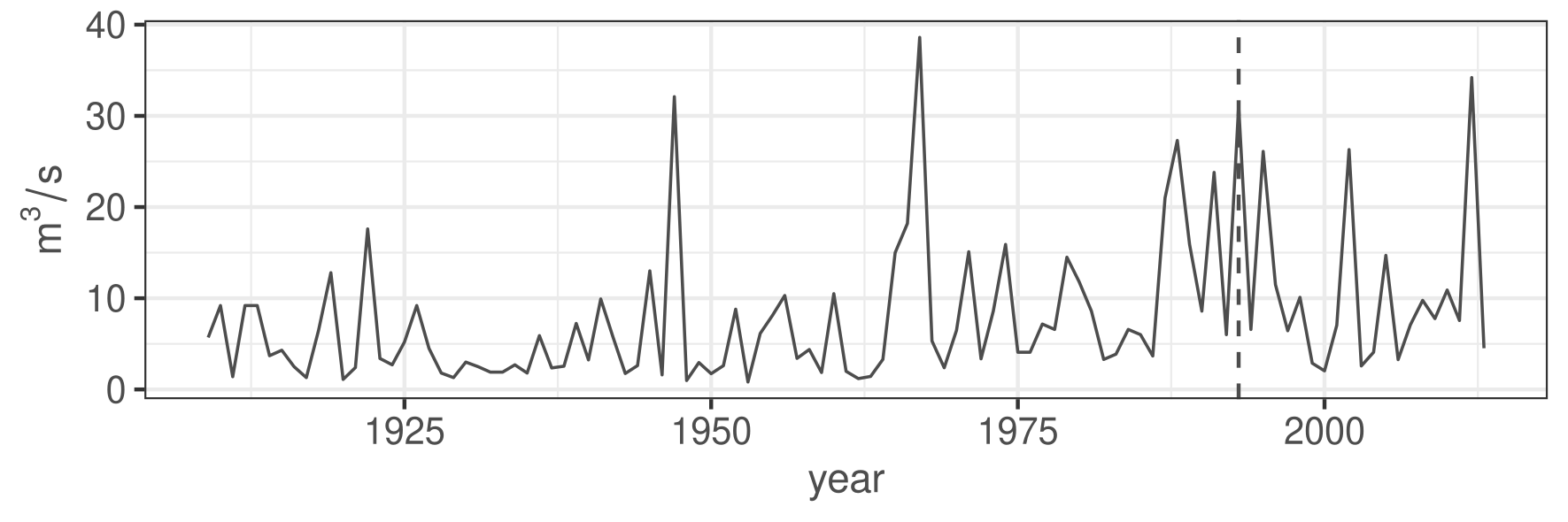
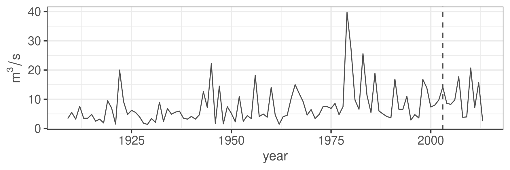
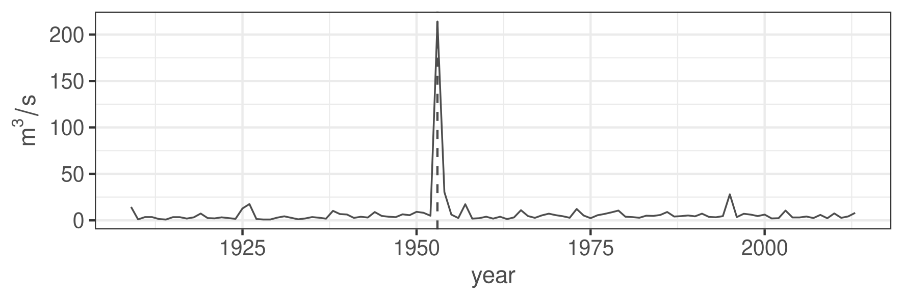
In this section, we illustrate potential applications of the new monitoring scheme in a data example. For this purpose, we consider a data set sampled in hydrology, which consists of the average daily flows measured in m3m^{3}/sec of the river Chemnitz at Göritzhain in Saxony, Germany, for the years 1909-2013.

This data has been previously analyzed in the (retrospective) change point literature by Sharipov et al., 2016, who developed methodology for detecting change points in functional data. The data set consists of a sample of n=105n=105 observations with dimension d=365d=365, such that each vector 𝑿t=(Xt,1,…,Xt,365)⊤\bm{X}_{t}=(X_{t,1},\dots,X_{t,365})^{\top} contains the daily average flows of one (German) hydrological year, which lasts from 1st of November to 31st of October. For instance, the data point X1,1X_{1,1} represents the daily average flow of the 1st of November 1909, while X105,365X_{105,365} is the same key figure for the 31st of October 2014. By this transformation, Sharipov et al., 2016 located a change in the annual flow curves in the year 1964. Dette and Gösmann, 2018 propose a retrospective test for relevant changes in a high dimensional time series. They consider the same data and locate 44 different mean changes that exceed a test threshold of 0.630.63 and are traced back to the dates 10th of July 1950, 18th of March 1956, 23rd of December 1965, 7th of February 1979, which correspond to spatial components 252252, 137137, 5353, 9999 , respectively.

Based on these prior analyses, we consider the first 35 observations as our initial stable data set and will use the remaining 70 observations as the monitoring period corresponding to a choice of m=35m=35 and T=2T=2. ¿From the initial set 𝑿1,…,𝑿35\bm{X}_{1},\dots,\bm{X}_{35} the spatial correlation structure is estimated via the implementation of the estimator based on the quadratic spectral kernel provided in the R-package ’sandwich’ [see Zeileis, 2004]. By the bootstrap in Algorithm A.1 the quantiles are obtained as q0.99=7.43q_{0.99}=7.43 and q0.95=4.93q_{0.95}=4.93, for which we conduct our monitoring method. During the monitoring period, we proceed as described in Algorithm A.1: If the detection scheme rejects the null hypothesis of no change at a certain time point, we report the corresponding component(s) as unstable and remove it/them from the sample. Afterwards, we continue monitoring with the remaining components until there is another rejection or the end of the monitoring period is attained.

The results of this procedure are displayed in Table 3 for the test levels α=0.01\alpha=0.01 and α=0.05\alpha=0.05 and can be summarized as follows. For a test level of 0.050.05 more unstable components (33) are identified than for 0.010.01 (17 components). Naturally, all breaks identified by the lower test level, are also detected by the other one, while the time of detection is sometimes earlier in the latter case. As the data exhibits (positive) spatial correlation, breaks partially occur in clusters, for example consider components 285, 286 and 287, for which both test levels detect changes or components 214, 215 and 216, for which changes are found at test level 0.050.05. Apparently, these clusters have to be considered as one change affecting several components, for instance a flood event or a new seasonal effect.

It is worth mentioning, that our findings match three out of four unstable components identified by the threshold procedure of Dette and Gösmann, 2018. Namely, we refer to components 53, 99, 252, which are likewise identified to contain a break by our sequential analysis. To illustrate the data set, we finally display the average daily flow over the years for these three components in Figure 3. The plots indicate that the break in component 252 (10th of July) is most probably caused by a huge outlier in the hydrological year starting in November 1953, which leads to an immediate rejection. This observation can be easily linked to a flood event in Saxony in summer of 1954 [see for instance Schröter et al., 2013]. For the components 53 (23rd of December) and 99 (7th of February), a visual inspection of the plots indicate actual structural changes.

α=0.05\alpha=0.05 α=0.01\alpha=0.01
component year component year component year component year
101 1945 54, 209 1995 101 1945 280 2009
252, 253 1953 264 1996 252, 253 1953 54, 215 2012
249, 251 1954 285, 286, 287 2001 249 1957 209 2013
247 1957 92 2002 105 1960
105 1960 99,192 2003 189 1977
189, 191 1977 138 2004 191 1979
104 1979 280, 283 2009 100 1980
100, 190 1980 44 2010 104 1986
102 1986 55, 214, 215, 216 2012 53 1995
53, 57 1993 199 2013 285, 286, 287 2001
Table 3: Structural breaks detected in the river flow data for a test level of α=0.05\alpha=0.05 (left column) and α=0.01\alpha=0.01 (right column). The column ’year’ specifies the (hydrological) year after which the rejection occurred. For instance 1945 means that the data from the hyrodological year 01st of November 1945 to 31st of October 1946 was already under consideration.
Refer to caption
Refer to caption
Refer to caption
Figure 3: Average daily flows for the dates 23rd of December (spatial component 53, upper row), 7th of February (spatial component 99, middle row) and 10th of July (spatial component 252, lower row). Vertical dashed lines indicate the time points at which a break was detected by the sequential method with a test level of 5%5\%.

Acknowledgments This work has been supported in part by the Collaborative Research Center “Statistical modeling of nonlinear dynamic processes” (SFB 823, Teilprojekt A1, C1) and the Research Training Group ’high-dimensional phenomena in probability - fluctuations and discontinuity’ (RTG 2131) of the German Research Foundation (DFG). The authors are grateful to Florian Heinrichs for extremely helpful discussions during the preparation of this manuscript and to Andreas Schumann and Svenja Fischer from the Institute of Engineering Hydrology and Water Resources Management of the Ruhr-Universität Bochum, who provided hydrological data analyzed in Section 4.2. Finally, we would like to thank all reviewers for their constructive comments on an earlier version of the manuscript.

References

  • Anatolyev and Kosenok, (2018) Anatolyev, S. and Kosenok, G. (2018). Sequential testing with uniformly distributed size. Journal of Time Series Econometrics, 10(2).
  • Andrews, (1991) Andrews, D. (1991). Heteroskedasticity and autocorrelation consistent covariance matrix estimation. Econometrica, 59(3):817–858.
  • Arratia et al., (1989) Arratia, R., Goldstein, L., and Gordon, L. (1989). Two moments suffice for Poisson approximations: The Chen-Stein method. The Annals of Probability, 17(1):9–25.
  • Aue et al., (2012) Aue, A., Hörmann, S., Horváth, L., Hušková, M., and Steinebach, J. G. (2012). Sequential testing for the stability of high-frequency portfolio betas. Econometric Theory, 28(4):804–837.
  • Aue and Horváth, (2004) Aue, A. and Horváth, L. (2004). Delay time in sequential detection of change. Statistics & Probability Letters, 67(3):221–231.
  • Aue et al., (2006) Aue, A., Horváth, L., Hušková, M., and Kokoszka, P. (2006). Change-point monitoring in linear models. The Econometrics Journal, 9(3):373–403.
  • Avanesov and Buzun, (2018) Avanesov, V. and Buzun, N. (2018). Change-point detection in high-dimensional covariance structure. Electronic Journal of Statistics, 12(2):3254–3294.
  • Berkes et al., (2014) Berkes, I., Liu, W., and Wu, W. B. (2014). Komlós-Major-Tusnády approximation under dependence. The Annals of Probability, 42(2):794–817.
  • Billingsley, (1999) Billingsley, P. (1999). Convergence of Probability Measures. Wiley Series in Probability and Statistics. John Wiley & Sons, Inc., New York, second edition.
  • Borodin and Salminen, (1996) Borodin, A. and Salminen, P. (1996). Handbook of Brownian Motion - Facts and Formulae. Probability and its applications. Birkhäuser, Basel.
  • Chen et al., (2020) Chen, Y., Wang, T., and Samworth, R. J. (2020). High-dimensional, multiscale online changepoint detection. arXiv e-print arXiv:2003.03668v1.
  • Chen and Tian, (2010) Chen, Z. and Tian, Z. (2010). Modified procedures for change point monitoring in linear models. Mathematics and Computers in Simulation, 81(1):62–75.
  • Chernozhukov et al., (2013) Chernozhukov, V., Chetverikov, D., and Kato, K. (2013). Gaussian approximations and multiplier bootstrap for maxima of sums of high-dimensional random vectors. The Annals of Statistics, 41(6):2786–2819.
  • Chernozhukov et al., (2019) Chernozhukov, V., Chetverikov, D., Kato, K., and Koike, Y. (2019). Improved central limit theorem and bootstrap approximations in high dimensions. arXiv e-print arXiv:1912.10529v1.
  • Cho and Fryzlewicz, (2015) Cho, H. and Fryzlewicz, P. (2015). Multiple-change-point detection for high dimensional time series via sparsified binary segmentation. Journal of the Royal Statistical Society: Series B (Statistical Methodology), 77(2):475–507.
  • Chochola et al., (2013) Chochola, O., Hušková, M., Prášková, Z., and Steinebach, J. G. (2013). Robust monitoring of capm portfolio betas. Journal of Multivariate Analysis, 115:374 – 395.
  • Chu et al., (1996) Chu, C.-S. J., Stinchcombe, M., and White, H. (1996). Monitoring structural change. Econometrica, 64(5):1045–1065.
  • Chu and Chen, (2018) Chu, L. and Chen, H. (2018). Sequential change-point detection for high-dimensional and non-euclidean data. arXiv e-print arXiv:1810.05973v1.
  • Ciuperca, (2013) Ciuperca, G. (2013). Two tests for sequential detection of a change-point in a nonlinear model. Journal of Statistical Planning and Inference, 143(10):1719–1743.
  • de Haan and Ferreira, (2006) de Haan, L. and Ferreira, A. (2006). Extreme Value Theory: An Introduction. Springer Series in Operations Research and Financial Engineering. Springer Science+Business Media, New York.
  • Dette et al., (2013) Dette, H., Bornkamp, B., and Bretz, F. (2013). On the efficiency of two-stage response-adaptive designs. Statistics in Medicine, 32(10):1646–1660.
  • Dette and Gösmann, (2018) Dette, H. and Gösmann, J. (2018). Relevant change points in high dimensional time series. Electronic Journal of Statistics, 12(2):2578–2636.
  • Dette and Gösmann, (2019) Dette, H. and Gösmann, J. (2019). A likelihood ratio approach to sequential change point detection for a general class of parameters. Journal of the American Statistical Association. Preprint available at: https://doi.org/10.1080/01621459.2019.1630562.
  • Dette et al., (2018) Dette, H., Pan, G. M., and Yang, Q. (2018). Estimating a change point in a sequence of very high-dimensional covariance matrices. arXiv e-print arXiv:1807.10797v1.
  • El Machkouri et al., (2013) El Machkouri, M., Volný, D., and Wu, W. B. (2013). A central limit theorem for stationary random fields. Stochastic Processes and their Applications, 123(1):1–14.
  • Embrechts et al., (1997) Embrechts, P., Klüppelberg, C., and Mikosch, T. (1997). Modelling Extremal Events for Insurance and Finance, volume 33 of Applications of Mathematics (New York). Springer, Berlin.
  • Enikeeva and Harchaoui, (2019) Enikeeva, F. and Harchaoui, Z. (2019). High-dimensional change-point detection under sparse alternatives. The Annals of Statistics, 47(4):2051–2079.
  • Feller, (1951) Feller, W. (1951). The asymptotic distribution of the range of sums of independent random variables. The Annals of Mathematical Statistics, 22(3):427–432.
  • Fremdt, (2014) Fremdt, S. (2014). Asymptotic distribution of the delay time in Page’s sequential procedure. Journal of Statistical Planning and Inference, 145:74–91.
  • Fremdt, (2015) Fremdt, S. (2015). Page’s sequential procedure for change-point detection in time series regression. Statistics, 49(1):128–155.
  • Gösmann et al., (2020) Gösmann, J., Kley, T., and Dette, H. (2020). A new approach for open-end sequential change point monitoring. To appear in: Journal of Time Series Analysis. Preprint available at https://doi.org/10.1111/jtsa.12555.
  • Hawkins et al., (2003) Hawkins, D. M., Qiu, P., and Kang, C. W. (2003). The changepoint model for statistical process control. Journal of Quality Technology, 35(4):355–366.
  • Hinkley, (1971) Hinkley, D. V. (1971). Inference about the change-point from cumulative sum tests. Biometrika, 58(3):509–523.
  • Hoga, (2017) Hoga, Y. (2017). Monitoring multivariate time series. Journal of Multivariate Analysis, 155:105–121.
  • Horváth et al., (2004) Horváth, L., Hušková, M., Kokoszka, P., and Steinebach, J. (2004). Monitoring changes in linear models. Journal of Statistical Planning and Inference, 126(1):225–251.
  • Hušková and Kirch, (2012) Hušková, M. and Kirch, C. (2012). Bootstrapping sequential change-point tests for linear regression. Metrika, 75(5):673–708.
  • Hušková and Koubková, (2005) Hušková, M. and Koubková, A. (2005). Monitoring jump changes in linear models. Journal of Statistical Research, 39(2):51–70.
  • Jiang, (2004) Jiang, T. (2004). The asymptotic distributions of the largest entries of sample correlation matrices. The Annals of Applied Probability, 14(2):865–880.
  • (39) Jirak, M. (2015a). Supplement to: Uniform change point tests in high dimension. The Annals of Statistics, 43(6):2451–2483. Supplement availabe at: https://doi.org/10.1214/15-AOS1347SUPP.
  • (40) Jirak, M. (2015b). Uniform change point tests in high dimension. The Annals of Statistics, 43(6):2451–2483.
  • Karatzas and Shreve, (1991) Karatzas, I. and Shreve, S. (1991). Brownian motion and stochastic calculus, volume 113 of Graduate Texts in Mathematics. Springer-Verlag, New York, second edition.
  • Kirch, (2008) Kirch, C. (2008). Bootstrapping sequential change-point tests. Sequential Analysis, 27(3):330–349.
  • Kirch and Kamgaing, (2015) Kirch, C. and Kamgaing, J. T. (2015). On the use of estimating functions in monitoring time series for change points. Journal of Statistical Planning and Inference, 161:25–49.
  • Kirch and Stoehr, (2019) Kirch, C. and Stoehr, C. (2019). Sequential change point tests based on U-statistics. arXiv e-print arXiv:1912.08580v1.
  • Kirch and Weber, (2018) Kirch, C. and Weber, S. (2018). Modified sequential change point procedures based on estimating functions. Electronic Journal of Statistics, 12(1):1579–1613.
  • Lai, (2001) Lai, T. L. (2001). Sequential analysis: Some classical problems and new challenges. Statistica Sinica, 11(2):303–351.
  • Lévy-Leduc and Roueff, (2009) Lévy-Leduc, C. and Roueff, F. (2009). Detection and localization of change-points in high-dimensional network traffic data. Annals of Applied Statistics, 3(2):637–662.
  • Liu et al., (2013) Liu, W., Xiao, H., and Wu, W. B. (2013). Probability and moment inequalities under dependence. Statistica Sinica, 23(3):1257–1272.
  • Mei, (2008) Mei, Y. (2008). Is average run length to false alarm always an informative criterion? Sequential Analysis, 27(4):354–376.
  • Mei, (2010) Mei, Y. (2010). Efficient scalable schemes for monitoring a large number of data streams. Biometrika, 97(2):419–433.
  • Moustakides, (1986) Moustakides, G. V. (1986). Optimal stopping times for detecting changes in distributions. The Annals of Statistics, 14(4):1379–1387.
  • Nikiforov, (1987) Nikiforov, I. (1987). Sequential detection of changes in stochastic systems. IFAC Proceedings Volumes, 20(2):321–327.
  • Otto and Breitung, (2019) Otto, S. and Breitung, J. (2019). Backward CUSUM for testing and monitoring structural change. arXiv e-print arXiv:2003.02682v1.
  • Page, (1954) Page, E. S. (1954). Continuous inspection schemes. Biometrika, 41(1/2):100–115.
  • Page, (1955) Page, E. S. (1955). Control charts with warning lines. Biometrika, 42(1/2):243–257.
  • Ross, (2014) Ross, G. J. (2014). Sequential change detection in the presence of unknown parameters. Statistics and Computing, 24(6):1017–1030.
  • Schröter et al., (2013) Schröter, K., Mühr, B., Elmer, F., Kunz-Plapp, T., and Trieselmann, W. (2013). June 2013 flood in central Europe - focus Germany. CEDIM Forensic Disaster Analysis Group (FDA). https://www.cedim.kit.edu/2850.php.
  • Serfling, (2009) Serfling, R. J. (2009). Approximation Theorems of Mathematical Statistics. Wiley Series in Probability and Statistics. John Wiley & Sons, Inc., New York.
  • Sharipov et al., (2016) Sharipov, O., Tewes, J., and Wendler, M. (2016). Sequential block bootstrap in a Hilbert space with application to change point analysis. The Canadian Journal of Statistics / La Revue Canadienne de Statistique, 44(3):300–322.
  • Soh and Chandrasekaran, (2017) Soh, Y. S. and Chandrasekaran, V. (2017). High-dimensional change-point estimation: Combining filtering with convex optimization. Applied and Computational Harmonic Analysis, 43(1):122–147.
  • Steland, (2006) Steland, A. (2006). A bootstrap view on Dickey-Fuller control charts for AR(1) series. Austrian Journal of Statistics, 35:339–346.
  • Tartakovsky et al., (2014) Tartakovsky, A., Nikiforov, I. V., and Basseville, M. (2014). Sequential Analysis: Hypothesis Testing and Changepoint Detection, volume 136 of Chapman & Hall/CRC Monographs on Statistics & Applied Probability. Chapman & Hall/CRC, Taylor and Francis Group.
  • Tartakovsky et al., (2006) Tartakovsky, A. G., Rozovskii, B. L., Blazek, R. B., and Hongjoong Kim (2006). A novel approach to detection of intrusions in computer networks via adaptive sequential and batch-sequential change-point detection methods. IEEE Transactions on Signal Processing, 54(9):3372–3382.
  • van der Vaart, (1998) van der Vaart, A. W. (1998). Asymptotic Statistics. Cambridge Series in Statistical and Probabilistic Mathematics. Cambridge University Press, Cambridge.
  • Wald, (1945) Wald, A. (1945). Sequential tests of statistical hypotheses. Annals of Mathematical Statistics, 16(2):117–186.
  • Wang et al., (2017) Wang, D., Yu, Y., and Rinaldo, A. (2017). Optimal covariance change point localization in high dimension. arXiv e-print arXiv:1712.09912v1.
  • Wang and Shao, (2020) Wang, R. and Shao, X. (2020). Dating the break in high-dimensional data. arXiv e-print arXiv:2002.04115v1.
  • Wang et al., (2019) Wang, R., Volgushev, S., and Shao, X. (2019). Inference for change points in high dimensional data. arXiv e-print arXiv:1905.08446v1.
  • (69) Wang, T. and Samworth, R. J. (2018a). High dimensional change point estimation via sparse projection. Journal of the Royal Statistical Society: Series B (Statistical Methodology), 80(1):57–83.
  • (70) Wang, T. and Samworth, R. J. (2018b). High dimensional change point estimation via sparse projection. Journal of the Royal Statistical Society: Series B (Statistical Methodology), 80(1):57–83.
  • Wied and Galeano, (2013) Wied, D. and Galeano, P. (2013). Monitoring correlation change in a sequence of random variables. Journal of Statistical Planning and Inference, 143(1):186–196.
  • Woodall and Montgomery, (1999) Woodall, W. H. and Montgomery, D. C. (1999). Research issues and ideas in statistical process control. Journal of Quality Technology, 31(4):376–386.
  • Wu, (2005) Wu, W. B. (2005). Nonlinear system theory: Another look at dependence. Proceedings of the National Academy of Sciences of the United States of America, 102(40):14150–14154.
  • Wu and Zhou, (2011) Wu, W. B. and Zhou, Z. (2011). Gaussian approximations for non-stationary multiple time series. Statistica Sinica, 21(3):1397–1413.
  • Xie and Siegmund, (2013) Xie, Y. and Siegmund, D. (2013). Sequential multi-sensor change-point detection. The Annals of Statistics, 41(2):670–692.
  • Yu et al., (2020) Yu, Y., Padilla, O. H. M., Wang, D., and Rinaldo, A. (2020). A note on online change point detection. arXiv e-print arXiv:2006.03283v1.
  • Zeileis, (2004) Zeileis, A. (2004). Econometric computing with HC and HAC covariance matrix estimators. Journal of Statistical Software, 11(10):1–17.
  • Zhang and Cheng, (2018) Zhang, X. and Cheng, G. (2018). Gaussian approximation for high dimensional vector under physical dependence. Bernoulli, 24(4A):2640–2675.
  • Zou et al., (2015) Zou, C., Wang, Z., Zi, X., and Jiang, W. (2015). An efficient online monitoring method for high-dimensional data streams. Technometrics, 57(3):374–387.

Appendix A Non-simultaneous changes among components

In this section, we present an algorithm to monitor for non-simultaneous change points in the mean vector of a high dimensional time series at test level α\alpha. For this purpose, we denote the set of all components without a change in the mean by

(A.1) 𝒮d:={h∈{1,…,d}|μ1,h=μ2,h=⋯=μm+T​m,h}.\displaystyle\mathcal{S}_{d}:=\big\{h\in\{1,\dots,d\}\;\big|\;\mu_{1,h}=\mu_{2,h}=\dots=\mu_{m+Tm,h}\big\}~.

For the complement set 𝒮dc={1,…,d}∖𝒮d\mathcal{S}_{d}^{c}=\{1,\dots,d\}\setminus\mathcal{S}_{d} let kh∗∈{1,…,m​T}k_{h}^{*}\in\{1,\ldots,mT\} denote the time of change in the component h∈𝒮dch\in\mathcal{S}_{d}^{c} within the monitoring period, that is

μ1,h=⋯=μm,h=⋯=μm+kh∗−1,h≠μm+kh∗,h=⋯=μm+T​m,h.\displaystyle\mu_{1,h}=\dots=\mu_{m,h}=\dots=\mu_{m+k_{h}^{*}-1,h}\neq\mu_{m+k_{h}^{*},h}=\dots=\mu_{m+Tm,h}~.

Note that, in this model, there is still at most one change point per component, however we allow the change times to be different among components. For what follows, recall the construction of the bootstrap statistic from Section 3.2. The algorithm below is capable of identifying the sets 𝒮d\mathcal{S}_{d} and 𝒮dc\mathcal{S}_{d}^{c}, see Theorem A.2 below.

Algorithm A.1

a

  1. Step 1:

    Either choose the quantile q1−αq_{1-\alpha} using the approximation by the Gumbel distribution, that is q1−α=g1−αq_{1-\alpha}=g_{1-\alpha}, where g1−αg_{1-\alpha} is the (1−α)(1-\alpha)-quantile of the Gumbel distribution or, alternatively, obtain the quantile from the bootstrap as follows:

    1. Step 1.1:

      Compute the long-run correlation estimates (ρ^i,j)i,j=1d\big(\hat{\rho}_{i,j}\big)_{i,j=1}^{d} from the initial set 𝑿1,…,𝑿m\bm{X}_{1},\dots,\bm{X}_{m}.

    2. Step 1.2:

      Based on these estimates, generate NN independent realizations of the Gaussian vectors (Z^t,1,…,Z^t,d)⊤(\widehat{Z}_{t,1},\ldots,\widehat{Z}_{t,d})^{\top} with covariance structure (ρ^i,j)i,j=1d\big(\hat{\rho}_{i,j}\big)_{i,j=1}^{d} for t=1,…,m+T​mt=1,\ldots,m+Tm and compute the corresponding bootstrap statistics

      ad​(𝒯^m,d(Z)​(1)−bd),ad​(𝒯^m,d(Z)​(2)−bd),…,ad​(𝒯^m,d(Z)​(N)−bd)a_{d}\big(\widehat{\mathcal{T}}_{m,d}^{(Z)}(1)-b_{d}\big),a_{d}\big(\widehat{\mathcal{T}}_{m,d}^{(Z)}(2)-b_{d}\big),\dots,a_{d}\big(\widehat{\mathcal{T}}_{m,d}^{(Z)}(N)-b_{d}\big)

      defined in (3.19).

    3. Step 1.3:

      Compute q1−αq_{1-\alpha} as the empirical (1−α)(1-\alpha)-quantile of the sample

      {ad​(𝒯^m,d(Z)​(n)−bd)}n=1,…,N.\Big\{a_{d}\Big(\widehat{\mathcal{T}}_{m,d}^{(Z)}(n)-b_{d}\Big)\Big\}_{n=1,\dots,N}~.
  2. Step 2:

    Initialize 𝒮^d,α:={1,…,d}\widehat{\mathcal{S}}_{d,\alpha}:=\{1,\dots,d\} and set k=1k=1.

    Monitoring: While k≤T​mk\leq Tm compute the statistics E^m,h​(k)\hat{E}_{m,h}(k). If the inequality

    maxh∈𝒮^d,α⁡w⁡(k/m)​E^m,h​(k)>q1−αad+bd\max_{h\in\widehat{\mathcal{S}}_{d,\alpha}}w(k/m)\hat{E}_{m,h}(k)>\dfrac{q_{1-\alpha}}{a_{d}}+b_{d}

    holds, reject the null hypothesis in favor of the alternative. Eliminate the components that led to the rejection, i.e.

    (A.2) 𝒮^d,α⟵𝒮^d,α∖{h∈𝒮^d,α|w⁡(k/m)​E^m,h​(k)>q1−αad+bd}\displaystyle\widehat{\mathcal{S}}_{d,\alpha}\longleftarrow\widehat{\mathcal{S}}_{d,\alpha}\setminus\Big\{h\in\widehat{\mathcal{S}}_{d,\alpha}\;\big|\;w(k/m)\hat{E}_{m,h}(k)>\dfrac{q_{1-\alpha}}{a_{d}}+b_{d}\,\Big\}

    and continue monitoring for k⟵k+1k\longleftarrow k+1 with the remaining components in 𝒮^d,α\widehat{\mathcal{S}}_{d,\alpha}.

  3. Step 3:

    If there was no rejection during monitoring, decide for the null hypothesis of no change in the mean vector. In case of rejections, decide for the alternative of a change in at least one component. Then, it holds that

    (A.3) 𝒮^d,α={h∈{1,…,d}|maxk=1T​m⁡w⁡(k/m)​E^m,h​(k)≤q1−αad+bd}\displaystyle\widehat{\mathcal{S}}_{d,\alpha}=\Big\{h\in\{1,\dots,d\}\;\;\Big|\;\;\max\limits_{k=1}^{Tm}w(k/m)\hat{E}_{m,h}(k)\leq\dfrac{q_{1-\alpha}}{a_{d}}+b_{d}\Big\}

    and the components remaining in this set are assumed as mean stable.

The following theorem states, that Algorithm A.1 is able to separate the sets 𝒮d\mathcal{S}_{d} and 𝒮dc\mathcal{S}_{d}^{c} correctly.

Theorem A.2

Let Assumptions 3.1-3.4 and 3.12 be satisfied and assume that Algorithm A.1 was launched either with the Gumbel or with the bootstrap quantile. The set 𝒮^d,α\widehat{\mathcal{S}}_{d,\alpha} defined in (A.3) satisfies

(A.4) lim supm,d→∞ℙ⁡(𝒮d⊂𝒮^d,α)≥1−α.\displaystyle\limsup_{m,d\to\infty}\,\mathbb{P}\Big(\mathcal{S}_{d}\subset\widehat{\mathcal{S}}_{d,\alpha}\Big)\geq 1-\alpha~.

If further

(A.5) mlog⁡m​minh∈𝒮dc​|μm+kh∗−1,h−μm+kh∗,h|→∞​and​lim supm,d→∞maxh∈𝒮dc⁡kh∗m<T,\displaystyle\sqrt{\dfrac{m}{\log m}}\,\min_{h\in\mathcal{S}_{d}^{c}}|\mu_{m+k_{h}^{*}-1,h}-\mu_{m+k_{h}^{*},h}|\to\infty\;\;\;\text{and}\;\;\;\limsup_{m,d\to\infty}\max_{h\in\mathcal{S}_{d}^{c}}\dfrac{k_{h}^{*}}{m}<T\,,

then

(A.6) limm,d→∞ℙ⁡(𝒮d⊃𝒮^d,α)=1.\displaystyle\lim_{m,d\to\infty}\mathbb{P}\Big(\mathcal{S}_{d}\supset\widehat{\mathcal{S}}_{d,\alpha}\Big)=1~.

By Theorem A.2, the set 𝒮^d,α\widehat{\mathcal{S}}_{d,\alpha} contains all the components without a change in the mean with high probability. It may also contain components in which the change in the mean is so small that it cannot be reliably detected. However, if we assume that that all changes in the mean are large enough and not too close to the monitoring end [see (A.5)], then 𝒮^d,α=𝒮d\widehat{\mathcal{S}}_{d,\alpha}=\mathcal{S}_{d} with high probability. That is, one detects all components exhibiting a change point without causing a false alarm.

Appendix B Proofs of main results

Let us first introduce some necessary notation, which will be frequently used throughout this section. The symbol ≲\lesssim denotes an inequality up to a constant, which does not depend on size mm of the training sample and the dimension dd. For two sequences ene_{n} and fnf_{n}, we write en∼fne_{n}\sim f_{n}, whenever fn/en→1f_{n}/e_{n}\to 1 as n→∞n\to\infty.

Let q∈(0,1]q\in(0,1]. By F𝕄F_{\mathbb{M}} we denote the distribution function of the range of a (standard) Brownian motion, that is 𝕄=maxt∈[0,q]⁡W⁡(t)−mint∈[0,q]⁡W⁡(t)\mathbb{M}=\max_{t\in[0,q]}W(t)-\min_{t\in[0,q]}W(t), which can be found in Borodin and Salminen, 1996, page 146, and is given by

F𝕄​(x)={1+4​∑k=1∞(−1)k​k​Erfc⁡(k​x2​q)if​x>0,0otherwise,\displaystyle F_{\mathbb{M}}(x)=\begin{cases}1+4\sum\limits_{k=1}^{\infty}(-1)^{k}k\Erfc\Big(\dfrac{kx}{\sqrt{2q}}\Big)\;\;&\text{if}\;\;x>0~,\\ 0&\text{otherwise}~,\end{cases}

where Erfc=1−Erf\Erfc=1-\Erf denotes the complementary error function. Using the elementary property Erf⁡(x)=2​Φ​(x​2)−1\Erf(x)=2\Phi(x\sqrt{2})-1 we obtain

(B.1) F𝕄​(x)=1+8​∑k=1∞(−1)k​k​Φ​(−k​xq)​for​x>0,\displaystyle F_{\mathbb{M}}(x)=1+8\sum_{k=1}^{\infty}(-1)^{k}k\Phi\Big(-\frac{kx}{\sqrt{q}}\Big)\;\;\text{for}\;x>0\,,

where throughout this paper Φ\Phi denotes the cumulative distribution function of a standard normal distribution.

B.1 Some preliminary results

We will begin with an auxiliary result. In Lemma B.1 we investigate the weak convergence of the maximum of independent identically distributed random variables with the same distribution as the random variable 𝕄\mathbb{M} defined in (2.7).

Lemma B.1

Let q∈(0,1]q\in(0,1] and M1′,M2′,…M_{1}^{\prime},M_{2}^{\prime},\ldots be independent identically distributed random variables with

M1′​=𝒟​max0≤t≤q⁡W⁡(t)−min0≤t≤q⁡W⁡(t),M_{1}^{\prime}\overset{\mathcal{D}}{=}\max_{0\leq t\leq q}W(t)-\min_{0\leq t\leq q}W(t)~,

where WW denotes a standard Brownian motion. Then, as d→∞d\to\infty, it holds that

ad​(maxh=1d​Mh′−bd)​⟹𝒟​G,\displaystyle a_{d}\Big(\max\limits_{h=1}^{d}M_{h}^{\prime}-b_{d}\Big)\overset{\mathcal{D}}{\Longrightarrow}G\,,

where GG is a standard Gumbel distributed random variable and ada_{d} and bdb_{d} are given by

(B.2) ad=2​log⁡dq and bd=2​q​log⁡d−q​(log⁡log⁡d−log⁡16π)2​2​log⁡d.a_{d}=\sqrt{\frac{2\log d}{q}}\quad\text{ and }\quad b_{d}=\sqrt{2q\log d}-\frac{\sqrt{q}\,(\log\log d-\log\tfrac{16}{\pi})}{2\sqrt{2\log d}}\,.
Proof of Lemma B.1.

The desired extreme value convergence will be derived from the distribution function of M1′M_{1}^{\prime}, which is given by F𝕄F_{\mathbb{M}} in (B.1). Observe, that F𝕄F_{\mathbb{M}} is twice differentiable with derivatives (for x>0x>0)

F𝕄′​(x)=4​2π​q​∑k=1∞(−1)k+1​k2​exp⁡(−k2​x22​q),\displaystyle F_{\mathbb{M}}^{\prime}(x)=\dfrac{4\sqrt{2}}{\sqrt{\pi q}}\sum_{k=1}^{\infty}(-1)^{k+1}k^{2}\exp\Big(-\dfrac{k^{2}x^{2}}{2q}\Big)~,
F𝕄′′​(x)=4​2π​q​q​∑k=1∞(−1)k​k4​x​exp⁡(−k2​x22​q),\displaystyle F_{\mathbb{M}}^{\prime\prime}(x)=\dfrac{4\sqrt{2}}{\sqrt{\pi q}q}\sum_{k=1}^{\infty}(-1)^{k}k^{4}x\exp\Big(-\dfrac{k^{2}x^{2}}{2q}\Big)~,

where we used that the series converge uniformly on all intervals [ε,∞)[\varepsilon,\infty) for ε>0\varepsilon>0 and therefore term by term differentiation is allowed. Thus, by Theorem 1.1.8 from de Haan and Ferreira, 2006 the distribution function F𝕄F_{\mathbb{M}} is in the domain of attraction of the Gumbel distribution if

(B.3) limx→∞(1−F𝕄​(x))​F𝕄′′​(x)(F𝕄′​(x))2=−1.\displaystyle\lim_{x\to\infty}\dfrac{(1-F_{\mathbb{M}}(x))F_{\mathbb{M}}^{\prime\prime}(x)}{(F_{\mathbb{M}}^{\prime}(x))^{2}}=-1\,.

Next, we prove (B.3). To this end, note that by the definition of the complimentary error function, we obtain for x>0x>0

(B.4) x⁡(1−F𝕄​(x))​exp⁡(x22​q)=4​∑k=1∞(−1)k+1​k​x​Erfc⁡(k​x2​q)​exp⁡(x22​q)=A1​(x)+A2​(x),\displaystyle\begin{split}x\big(1-F_{\mathbb{M}}(x)\big)\exp\Big(\dfrac{x^{2}}{2q}\Big)&=4\sum\limits_{k=1}^{\infty}(-1)^{k+1}kx\Erfc\Big(\dfrac{kx}{\sqrt{2q}}\Big)\exp\Big(\dfrac{x^{2}}{2q}\Big)\\ &=A_{1}(x)+A_{2}(x)\,,\end{split}

where the two summands on the right-hand side are given by

A1​(x)\displaystyle A_{1}(x) =8π​∫x2​q∞exp⁡(−τ2)​𝑑τ⋅x​exp⁡(x22​q),\displaystyle=\dfrac{8}{\sqrt{\pi}}\int_{\frac{x}{\sqrt{2q}}}^{\infty}\exp(-\tau^{2})d\tau\cdot x\exp\Big(\dfrac{x^{2}}{2q}\Big)~,
A2​(x)\displaystyle A_{2}(x) =8π​∑k=2∞(−1)k+1​k​x​∫k​x2​q∞exp⁡(−τ2)​𝑑τ⋅exp⁡(x22​q).\displaystyle=\dfrac{8}{\sqrt{\pi}}\sum\limits_{k=2}^{\infty}(-1)^{k+1}kx\int_{\frac{kx}{\sqrt{2q}}}^{\infty}\exp(-\tau^{2})d\tau\cdot\exp\Big(\dfrac{x^{2}}{2q}\Big)~.

We will treat the two summands of the last display separately. For the first summand we obtain that

limx→∞A1​(x)=\displaystyle\lim_{x\to\infty}A_{1}(x)= 8π​limx→∞∫x2​q∞exp⁡(−τ2)​𝑑τx−1​exp⁡(−x22​q)\displaystyle\dfrac{8}{\sqrt{\pi}}\lim_{x\to\infty}\frac{\int_{\frac{x}{\sqrt{2q}}}^{\infty}\exp(-\tau^{2})d\tau}{x^{-1}\exp\Big(\dfrac{-x^{2}}{2q}\Big)}
=\displaystyle= 8π​limx→∞−12​q​exp⁡(−x22​q)−x−2​exp⁡(−x22​q)−1q​exp⁡(−x22​q)=4​2​qπ\displaystyle\dfrac{8}{\sqrt{\pi}}\lim_{x\to\infty}\frac{\dfrac{-1}{\sqrt{2q}}\exp\Big(\dfrac{-x^{2}}{2q}\Big)}{-x^{-2}\exp\Big(\dfrac{-x^{2}}{2q}\Big)-\frac{1}{q}\exp\Big(\dfrac{-x^{2}}{2q}\Big)}=4\dfrac{\sqrt{2q}}{\sqrt{\pi}}

by L’Hôspital’s rule. For the second summand of the last display in (B.4) note that

|π8​A2​(x)|\displaystyle\Big|\dfrac{\sqrt{\pi}}{8}A_{2}(x)\Big| ≤∑k=2∞k​x​∫k​x2​q∞exp⁡(−τ2)​𝑑τ⋅exp⁡(x22​q)\displaystyle\leq\sum\limits_{k=2}^{\infty}kx\int_{\frac{kx}{\sqrt{2q}}}^{\infty}\exp(-\tau^{2})d\tau\cdot\exp\Big(\dfrac{x^{2}}{2q}\Big)
≤2​q​∑k=2∞∫k​x2​q∞τ​exp⁡(−τ2)​𝑑τ⋅exp⁡(x22​q)\displaystyle\leq\sqrt{2q}\sum\limits_{k=2}^{\infty}\int_{\frac{kx}{\sqrt{2q}}}^{\infty}\tau\exp(-\tau^{2})d\tau\cdot\exp\Big(\dfrac{x^{2}}{2q}\Big)
=q2​exp⁡(−x22​q)​∑k=2∞exp⁡(−(k2−2)​x22​q)\displaystyle=\sqrt{\dfrac{q}{2}}\exp\Big(\dfrac{-x^{2}}{2q}\Big)\sum\limits_{k=2}^{\infty}\exp\Big(-\frac{(k^{2}-2)x^{2}}{2q}\Big)
≤(x≥1)​q2​exp⁡(−x22​q)​∑k=2∞exp⁡(−k2−22​q)=o⁡(1)​as​x→∞.\displaystyle\overset{(x\geq 1)}{\leq}\sqrt{\dfrac{q}{2}}\exp\bigg(\dfrac{-x^{2}}{2q}\bigg)\sum\limits_{k=2}^{\infty}\exp\bigg(-\frac{k^{2}-2}{2q}\bigg)=o(1)\;\;\text{as}\;\;x\to\infty~.

Combining the last statements with the decomposition in (B.4) yields

(B.5) limx→∞x⁡(1−F𝕄​(x))​exp⁡(x22​q)=4​2​qπ.\displaystyle\lim_{x\to\infty}x\big(1-F_{\mathbb{M}}(x)\big)\exp\Big(\dfrac{x^{2}}{2q}\Big)=4\dfrac{\sqrt{2q}}{\sqrt{\pi}}~.

For the denominator of (B.3) note that

(B.6) limx→∞F𝕄′​(x)​exp⁡(x22​q)=4​2π​q+limx→∞4​2π​q​∑k=2∞(−1)k+1​k2​exp⁡(−(k2−1)​x22​q)=4​2π​q,\displaystyle\begin{split}\lim_{x\to\infty}F_{\mathbb{M}}^{\prime}(x)\exp\Big(\dfrac{x^{2}}{2q}\Big)&=\dfrac{4\sqrt{2}}{\sqrt{\pi q}}+\lim_{x\to\infty}\dfrac{4\sqrt{2}}{\sqrt{\pi q}}\sum_{k=2}^{\infty}(-1)^{k+1}k^{2}\exp\Big(-\dfrac{(k^{2}-1)x^{2}}{2q}\Big)\\ &=\dfrac{4\sqrt{2}}{\sqrt{\pi q}}~,\end{split}

where we used that for x≥1x\geq 1

∑k=2∞k2​exp⁡(−(k2−1)​x22​q)\displaystyle\sum_{k=2}^{\infty}k^{2}\exp\Big(-\dfrac{(k^{2}-1)x^{2}}{2q}\Big) ≤exp⁡(−x22​q)​∑k=2∞k2​exp⁡(−(k2−2)2​q)=o⁡(1)​as​x→∞.\displaystyle\leq\exp\Big(\dfrac{-x^{2}}{2q}\Big)\sum_{k=2}^{\infty}k^{2}\exp\Big(-\dfrac{(k^{2}-2)}{2q}\Big)=o(1)\;\;\text{as}\;\;x\to\infty~.

Using similar arguments we obtain

(B.7) limx→∞x−1​F𝕄′′​(x)​exp⁡(x22​q)=−4​2π​q​q+limx→∞4​2π​q​q​∑k=2∞(−1)k​k4​exp⁡(−x2​(k2−1)2​q)=−4​2π​q​q.\displaystyle\begin{split}\lim_{x\to\infty}&x^{-1}F_{\mathbb{M}}^{\prime\prime}(x)\exp\Big(\dfrac{x^{2}}{2q}\Big)\\ =&\dfrac{-4\sqrt{2}}{\sqrt{\pi q}q}+\lim_{x\to\infty}\dfrac{4\sqrt{2}}{\sqrt{\pi q}q}\sum_{k=2}^{\infty}(-1)^{k}k^{4}\exp\Big(-\dfrac{x^{2}(k^{2}-1)}{2q}\Big)=\dfrac{-4\sqrt{2}}{\sqrt{\pi q}q}~.\end{split}

Combining (B.5), (B.6) and (B.7), it follows that

limx→∞(1−F𝕄​(x))​F𝕄′′​(x)(F𝕄′​(x))2=limx→∞x⁡(1−F𝕄​(x))​exp⁡(x22​q)​limx→∞x−1​F𝕄′′​(x)​exp⁡(x22​q)limx→∞(F𝕄′​(x)​exp⁡(x22​q))2=−1,\displaystyle\lim_{x\to\infty}\dfrac{(1-F_{\mathbb{M}}(x))F_{\mathbb{M}}^{\prime\prime}(x)}{(F_{\mathbb{M}}^{\prime}(x))^{2}}=\frac{\lim\limits_{x\to\infty}x(1-F_{\mathbb{M}}(x))\exp\Big(\dfrac{x^{2}}{2q}\Big)\lim\limits_{x\to\infty}x^{-1}F_{\mathbb{M}}^{\prime\prime}(x)\exp\Big(\dfrac{x^{2}}{2q}\Big)}{\lim\limits_{x\to\infty}\Big(F_{\mathbb{M}}^{\prime}(x)\exp\Big(\dfrac{x^{2}}{2q}\Big)\Big)^{2}}=-1,

which completes the proof of (B.3). By definition of the maximum domain of attraction, (B.3) is equivalent to the existence of sequences ad>0,bda_{d}>0,b_{d} such that

ad​(maxh=1d​Mh′−bd)​⟹𝒟​G​as​d→∞.\displaystyle a_{d}\Big(\max\limits_{h=1}^{d}M_{h}^{\prime}-b_{d}\Big)\overset{\mathcal{D}}{\Longrightarrow}G\;\;\text{as}\;\;d\to\infty~.

Our next goal is to find an explicit formula for these sequences, for which we will employ Proposition 3.3.28 in Embrechts et al., 1997. Therefore consider the distribution function

H(x):=1−42​qπx−1exp(−x2/(2q),x>x0.H(x):=1-4\frac{\sqrt{2q}}{\sqrt{\pi}}x^{-1}\exp\big(-x^{2}/(2q\big)\,,\qquad x>x_{0}~.

Note that we can rewrite equation (B.5) as

(B.8) limx→∞(1−F𝕄(x))(42​qπx−1exp(−x2/(2q))−1=1\lim_{x\to\infty}(1-F_{\mathbb{M}}(x))\Big(4\frac{\sqrt{2q}}{\sqrt{\pi}}x^{-1}\exp\big(-x^{2}/(2q\big)\Big)^{-1}=1\,

and thereby obtain the tail-equivalence

limx→∞1−F𝕄​(x)1−H⁡(x)=1.\lim_{x\to\infty}\frac{1-F_{\mathbb{M}}(x)}{1-H(x)}=1\,.

Thus, by Proposition 3.3.28 in Embrechts et al., 1997 we have to find sequences ad,bda_{d},b_{d} such that limd→∞Hd​(ad−1​x+bd)=FG​(x)\lim_{d\to\infty}H^{d}(a_{d}^{-1}x+b_{d})=F_{G}(x) for all x∈ℝx\in\mathbb{R}. Since HH has Weibull-like tails, a possible choice of the norming sequences is given in Table 3.4.4 in Embrechts et al., 1997:

bd\displaystyle b_{d} =2​q​log⁡d+12​2​q​log⁡d​(−q​log⁡(2​q​log⁡d)+2​q​log⁡32​qπ)\displaystyle=\sqrt{2q\log d}+\frac{1}{2\sqrt{2q\log d}}\Big(-q\log\big(2q\log d\big)+2q\log\sqrt{\frac{32q}{\pi}}\Big)
ad−1\displaystyle a_{d}^{-1} =q(2qlogd)−1/2.\displaystyle=q(2q\log d)^{-1/2}\,.

After simplification we get the desired result

(B.9) ad=2​log⁡dq and bd=2​q​log⁡d−q​(log⁡log⁡d−log⁡16π)2​2​log⁡d,a_{d}=\sqrt{\frac{2\log d}{q}}\quad\text{ and }\quad b_{d}=\sqrt{2q\log d}-\frac{\sqrt{q}\,(\log\log d-\log\tfrac{16}{\pi})}{2\sqrt{2\log d}}\,,

which finishes the proof of Lemma B.1. ∎

B.2 Proof of Theorem 3.5

Let q∈(0,1]q\in(0,1] and recall the definition of MhM_{h} in Theorem 3.5. By Theorem 1 from Arratia et al., 1989 in the form as presented in Lemma A.4 in Jiang, 2004 we obtain for any x∈ℝx\in\mathbb{R} the inequality

(B.10) |ℙ⁡(maxh=1d​Mh≤ud​(x))−exp⁡(−λ)|≤(1∧λ−1)​(Λ1+Λ2+Λ3),\displaystyle\left|\mathbb{P}\left(\max\limits_{h=1}^{d}M_{h}\leq u_{d}(x)\right)-\exp(-\lambda)\right|\leq\big(1\wedge\lambda^{-1})(\Lambda_{1}+\Lambda_{2}+\Lambda_{3}\big)~,

with λ=∑h=1dℙ⁡(Mh>ud​(x))\lambda=\sum_{h=1}^{d}\mathbb{P}\big(M_{h}>u_{d}(x)\big) and

Λ1\displaystyle\Lambda_{1} =∑i=1d∑1≤j≤d|i−j|≤Ldℙ⁡(Mi>ud​(x))​ℙ​(Mj>ud​(x)),\displaystyle=\sum_{i=1}^{d}\sum_{\begin{subarray}{c}1\leq j\leq d\\ |i-j|\leq L_{d}\end{subarray}}\mathbb{P}\big(M_{i}>u_{d}(x)\big)\mathbb{P}\big(M_{j}>u_{d}(x)\big)~,
Λ2\displaystyle\Lambda_{2} =∑i=1d∑1≤j≤dj≠i,|i−j|≤Ldℙ⁡(Mi>ud​(x),Mj>ud​(x)),\displaystyle=\sum_{i=1}^{d}\sum_{\begin{subarray}{c}1\leq j\leq d\\ j\neq i,\,|i-j|\leq L_{d}\end{subarray}}\mathbb{P}\big(M_{i}>u_{d}(x),M_{j}>u_{d}(x)\big)~,
Λ3\displaystyle\Lambda_{3} =∑i=1d𝔼|ℙ(Mi>ud(x)|σ(Mj:|i−j|>Ld))−ℙ(Mi>ud(x))|,\displaystyle=\sum_{i=1}^{d}\mathbb{E}\left|\mathbb{P}\Big(M_{i}>u_{d}(x)\,|\,\sigma\big(M_{j}:|i-j|>L_{d}\big)\Big)-\mathbb{P}(M_{i}>u_{d}(x)\big)\right|~,

where ud​(x)=x/ad+bdu_{d}(x)=x/a_{d}+b_{d} and σ(Mj:|i−j|>Ld)\sigma\big(M_{j}:|i-j|>L_{d}\big) denotes the σ\sigma-algebra generated by the set {Mj:|i−j|>Ld}\big\{M_{j}:|i-j|>L_{d}\big\}. In the remainder of the proof we fix x∈ℝx\in\mathbb{R} and due to ad,bd→∞a_{d},\,b_{d}\to\infty we can assume that dd is sufficiently large such that ud​(x)>0u_{d}(x)>0. Further let M1′,M2′,…M_{1}^{\prime},M_{2}^{\prime},\ldots be i.i.d. random variables with M1′​=𝒟​M1M_{1}^{\prime}\overset{\mathcal{D}}{=}M_{1}. With Lemma B.1 we have

(B.11) limd→∞ℙ⁡(maxh=1d​Mh′≤ud​(x))=limd→∞(ℙ⁡(M1≤ud​(x)))d=exp⁡(−exp⁡(−x)).\displaystyle\lim_{d\to\infty}\mathbb{P}\Big(\max\limits_{h=1}^{d}M_{h}^{\prime}\leq u_{d}(x)\Big)=\lim_{d\to\infty}\Big(\mathbb{P}\big(M_{1}\leq u_{d}(x)\big)\Big)^{d}=\exp\big(-\exp(-x)\big)~.

As bd→∞b_{d}\rightarrow\infty and limx→0xlog⁡(1−x)=−1\lim\limits_{x\rightarrow 0}\frac{x}{\log(1-x)}=-1, (B.11) yields

(B.12) λ=∑h=1dℙ⁡(Mh>ud​(x))=d​ℙ​(M1>ud​(x))=−d​log⁡(1−ℙ⁡(M1>ud​(x)))​(1+o⁡(1))=−(log⁡(ℙ​(M1≤ud​(x))d))​(1+o⁡(1))→exp⁡(−x)as ​d→∞.\displaystyle\begin{split}\lambda=&\sum_{h=1}^{d}\mathbb{P}\big(M_{h}>u_{d}(x)\big)=d\mathbb{P}\big(M_{1}>u_{d}(x)\big)\\ =&-d\log\left(1-\mathbb{P}\big(M_{1}>u_{d}(x)\big)\right)\big(1+o(1)\big)\\ =&-\left(\log\left(\mathbb{P}(M_{1}\leq u_{d}(x))^{d}\right)\right)\big(1+o(1)\big)\rightarrow\exp(-x)\quad\mbox{as }d\rightarrow\infty~.\end{split}

To treat Λ1\Lambda_{1}, note that (B.12) yields for d→∞d\to\infty

(B.13) 1−F𝕄​(ud​(x))∼exp⁡(−x)d.\displaystyle 1-F_{\mathbb{M}}(u_{d}(x))\sim\dfrac{\exp(-x)}{d}~.

Since Ld=o⁡(d)L_{d}=o(d) by assumption, we obtain

(B.14) Λ1=2​d​Ld​(1−F𝕄​(ud​(x)))2\displaystyle\Lambda_{1}=2dL_{d}\big(1-F_{\mathbb{M}}(u_{d}(x))\big)^{2} ∼2​Ldd​exp⁡(−2​x)=o⁡(1).\displaystyle\sim 2\dfrac{L_{d}}{d}\exp(-2x)=o(1)~.

To derive the asymptotic properties of Λ2\Lambda_{2}, observe the bound

(B.15) Λ2≤2​d​Ld​max1≤i<j≤dρi,j=0,|i−j|≤Ld,⁡ℙ⁡(Mi>ud​(x),Mj>ud​(x))+2​d​Ld​max1≤i<j≤dρi,j≠0,|i−j|≤Ld,⁡ℙ⁡(Mi>ud​(x),Mj>ud​(x)),\displaystyle\begin{split}\Lambda_{2}&\leq 2dL_{d}\max_{\begin{subarray}{c}1\leq i<j\leq d\\ \rho_{i,j}=0,\,|i-j|\leq L_{d},\end{subarray}}\mathbb{P}\big(M_{i}>u_{d}(x),M_{j}>u_{d}(x)\big)\\ &\quad+2dL_{d}\max_{\begin{subarray}{c}1\leq i<j\leq d\\ \rho_{i,j}\neq 0,\,|i-j|\leq L_{d},\end{subarray}}\mathbb{P}\big(M_{i}>u_{d}(x),M_{j}>u_{d}(x)\big),\end{split}

where throughout this proof we write ρi,j\rho_{i,j} instead of ρi,j(d)\rho_{i,j}^{(d)} for simplicity. Note, that in case of ρi,j=0\rho_{i,j}=0 it holds by (B.13), as d→∞d\to\infty ,

ℙ⁡(Mi>ud​(x),Mj>ud​(x))\displaystyle\mathbb{P}\big(M_{i}>u_{d}(x),M_{j}>u_{d}(x)\big) =(ℙ⁡(M1>ud​(x)))2∼(exp⁡(−x)d)2,\displaystyle=\big(\mathbb{P}\big(M_{1}>u_{d}(x))\big)^{2}\sim\left(\frac{\exp(-x)}{d}\right)^{2}~,

which implies that the first summand on the right-hand side in (B.15) vanishes. To treat the other one, we follow the idea in Lemma B.11 from Jirak, 2015a and use that a comparison of the covariance structures of the two Gaussian processes yields

{(Wi​(t),Wj​(t))}t≥0​=𝒟​{(Wi​(t),1−ρi,j2​Wj′​(t)+ρi,j​Wi​(t))}t≥0,\displaystyle\Big\{\big(W_{i}(t),W_{j}(t)\big)\Big\}_{t\geq 0}\overset{\mathcal{D}}{=}\Big\{\left(W_{i}(t),\sqrt{1-\rho_{i,j}^{2}}W_{j}^{\prime}(t)+\rho_{i,j}W_{i}(t)\right)\Big\}_{t\geq 0}~,

where Wj′W_{j}^{\prime} is a standard Wiener process that is independent of WiW_{i}. Consequently, it also holds that

(Mi,Mj)​=𝒟​(Mi,sup0≤t≤qsup0≤s≤t|1−ρi,j2​(Wj′​(t)−Wj′​(s))+ρi,j​(Wi​(t)−Wi​(s))|)\displaystyle\left(M_{i},\,M_{j}\right)\overset{\mathcal{D}}{=}\left(M_{i},\sup_{0\leq t\leq q}\sup_{0\leq s\leq t}\left|\sqrt{1-\rho_{i,j}^{2}}\big(W_{j}^{\prime}(t)-W_{j}^{\prime}(s)\big)+\rho_{i,j}\big(W_{i}(t)-W_{i}(s)\big)\right|\right)

and by the triangle inequality

sup0≤t≤qsup0≤s≤t|1−ρi,j2​(Wj′​(t)−Wj′​(s))+ρi,j​(Wi​(t)−Wi​(s))|\displaystyle\sup_{0\leq t\leq q}\sup_{0\leq s\leq t}\left|\sqrt{1-\rho_{i,j}^{2}}\big(W_{j}^{\prime}(t)-W_{j}^{\prime}(s)\big)+\rho_{i,j}\big(W_{i}(t)-W_{i}(s)\big)\right|
≤1−ρi,j2​sup0≤t≤qsup0≤s≤t|Wj′​(t)−Wj′​(s)|+|ρi,j|​sup0≤t≤qsup0≤s≤t|Wi​(t)−Wi​(s)|\displaystyle\leq\sqrt{1-\rho_{i,j}^{2}}\sup_{0\leq t\leq q}\sup_{0\leq s\leq t}\left|W_{j}^{\prime}(t)-W_{j}^{\prime}(s)\right|+|\rho_{i,j}|\sup_{0\leq t\leq q}\sup_{0\leq s\leq t}\left|W_{i}(t)-W_{i}(s)\right|
=𝒟​1−ρi,j2​Mj′+|ρi,j|​Mi,\displaystyle\overset{\mathcal{D}}{=}\sqrt{1-\rho_{i,j}^{2}}M_{j}^{\prime}+|\rho_{i,j}|M_{i}~,

where Mj′M_{j}^{\prime} has the same distribution as MjM_{j} but is independent of MiM_{i}. Now, we obtain for δ∈(0,1)\delta\in(0,1) and ε=δ⁡(1|ρi,j|−1)\varepsilon=\delta\big(\tfrac{1}{|\rho_{i,j}|}-1\big),

ℙ(Mi>ud(x),Mj>ud(x))≤ℙ(Mi>ud(x),1−ρi,j2Mj′+|ρi,j|Mi>ud(x))\displaystyle\mathbb{P}\big(M_{i}>u_{d}(x),M_{j}>u_{d}(x)\big)\leq\mathbb{P}\left(M_{i}>u_{d}(x),\sqrt{1-\rho_{i,j}^{2}}M_{j}^{\prime}+|\rho_{i,j}|M_{i}>u_{d}(x)\right)
=∫ud​(x)∞ℙ⁡(Mj′≥ud​(x)−y​|ρi,j|1−ρi,j2)​ℙMi​(𝑑y)\displaystyle=\int_{u_{d}(x)}^{\infty}\mathbb{P}\left(M_{j}^{\prime}\geq\frac{u_{d}(x)-y|\rho_{i,j}|}{\sqrt{1-\rho_{i,j}^{2}}}\right)\mathbb{P}_{M_{i}}(dy)
≤∫ud​(x)ud​(x)​(1|ρi,j|−ε)ℙ⁡(Mj′≥ud​(x)−y​|ρi,j|1−ρi,j2)​ℙMi​(𝑑y)+ℙ⁡(Mi>ud​(x)​(1|ρi,j|−ε))\displaystyle\leq\int_{u_{d}(x)}^{u_{d}(x)\big(\frac{1}{|\rho_{i,j}|}-\varepsilon\big)}\mathbb{P}\left(M_{j}^{\prime}\geq\frac{u_{d}(x)-y|\rho_{i,j}|}{\sqrt{1-\rho_{i,j}^{2}}}\right)\mathbb{P}_{M_{i}}(dy)+\mathbb{P}\Big(M_{i}>u_{d}(x)\big(\tfrac{1}{|\rho_{i,j}|}-\varepsilon\big)\Big)
:=Pi​j(1)+Pi​j(2).\displaystyle:=P_{ij}^{(1)}+P_{ij}^{(2)}\,.

First, we bound Pi​j(2)P_{ij}^{(2)}. To this end, recall from (B.5) that

(B.16) ℙ(M1>x)∼Kx−1exp(−x2/(2q)),x→∞,\mathbb{P}(M_{1}>x)\sim Kx^{-1}\exp(-x^{2}/(2q))\,,\qquad x\to\infty~,

where K=4​2​qπK=4\frac{\sqrt{2q}}{\sqrt{\pi}}. By |ρi,j|≤ρ+<1|\rho_{i,j}|\leq\rho_{+}<1 we obtain

(B.17) Pi​j(2)=ℙ⁡(Mi>ud​(x)​(1|ρi,j|​(1−δ)+δ))≤ℙ⁡(Mi>ud​(x)​(1ρ+​(1−δ)+δ))∼K​1ud​(x)​(1ρ+​(1−δ)+δ)​exp⁡(−ud​(x)22​q​(1ρ+​(1−δ)+δ)2)≤12​exp⁡(−ud​(x)22​q​(ρ+−1​(1−δ)+δ)2),\displaystyle\begin{split}P_{ij}^{(2)}&=\mathbb{P}\Big(M_{i}>u_{d}(x)\big(\tfrac{1}{|\rho_{i,j}|}(1-\delta)+\delta\big)\Big)\leq\mathbb{P}\Big(M_{i}>u_{d}(x)\big(\tfrac{1}{\rho_{+}}(1-\delta)+\delta\big)\Big)\\ &\sim K\frac{1}{u_{d}(x)\big(\tfrac{1}{\rho_{+}}(1-\delta)+\delta\big)}\exp\Big(-\frac{u_{d}(x)^{2}}{2q}\big(\tfrac{1}{\rho_{+}}(1-\delta)+\delta\big)^{2}\Big)\\ &\leq\frac{1}{2}\exp\Big(-\frac{u_{d}(x)^{2}}{2q}\big(\rho_{+}^{-1}(1-\delta)+\delta\big)^{2}\Big)\,,\end{split}

where the last inequality holds for sufficiently large dd depending on ρ+\rho_{+} since ud​(x)→∞u_{d}(x)\to\infty. As regards Pi​j(1)P_{ij}^{(1)}, we have

Pi​j(1)\displaystyle P_{ij}^{(1)} ≤ℙ⁡(M1>ud​(x))​ℙ​(M1>ud​(x)​ε​|ρi,j|1−ρi,j2)\displaystyle\leq\mathbb{P}\big(M_{1}>u_{d}(x)\big)\,\mathbb{P}\Big(M_{1}>u_{d}(x)\tfrac{\varepsilon|\rho_{i,j}|}{\sqrt{1-\rho_{i,j}^{2}}}\Big)
=ℙ⁡(M1>ud​(x))​ℙ​(M1>ud​(x)​δ​1−|ρi,j|1−ρi,j2)≤ℙ⁡(M1>ud​(x))​ℙ​(M1>ud​(x)​δ​1−ρ+1−ρ+2),\displaystyle=\mathbb{P}\big(M_{1}>u_{d}(x)\big)\,\mathbb{P}\Big(M_{1}>u_{d}(x)\delta\tfrac{1-|\rho_{i,j}|}{\sqrt{1-\rho_{i,j}^{2}}}\Big)\leq\mathbb{P}\big(M_{1}>u_{d}(x)\big)\,\mathbb{P}\Big(M_{1}>u_{d}(x)\delta\tfrac{1-\rho_{+}}{\sqrt{1-\rho_{+}^{2}}}\Big)~,

where we used that the map x↦(1−x)/1−x2x\mapsto(1-x)/\sqrt{1-x^{2}} is decreasing on [0,1)[0,1). Employing again (B.16), we conclude for sufficiently large dd

(B.18) ℙ⁡(M1>ud​(x))​ℙ​(M1>ud​(x)​δ​1−ρ+1−ρ+2)∼K2​1−ρ+2ud​(x)2​δ​(1−ρ+)​exp⁡(−ud​(x)22​q​(1+δ2​(1−ρ+)21−ρ+2))≤12​exp⁡(−ud​(x)22​q​(1+δ2​(1−ρ+)2)).\displaystyle\begin{split}\mathbb{P}\big(M_{1}>u_{d}(x)\big)\,\mathbb{P}\Big(M_{1}>u_{d}(x)\delta\tfrac{1-\rho_{+}}{\sqrt{1-\rho_{+}^{2}}}\Big)&\sim K^{2}\frac{\sqrt{1-\rho_{+}^{2}}}{u_{d}(x)^{2}\delta(1-\rho_{+})}\exp\left(-\frac{u_{d}(x)^{2}}{2q}\left(1+\tfrac{\delta^{2}(1-\rho_{+})^{2}}{1-\rho_{+}^{2}}\right)\right)\\ &\leq\frac{1}{2}\exp\left(-\frac{u_{d}(x)^{2}}{2q}\left(1+\delta^{2}(1-\rho_{+})^{2}\right)\right)\,.\end{split}

Combining (B.17) and (B.18) we get

ℙ⁡(Mi>ud​(x),Mj>ud​(x))\displaystyle\mathbb{P}\big(M_{i}>u_{d}(x),M_{j}>u_{d}(x)\big) ≤exp⁡(−ud​(x)22​q​min⁡(f⁡(δ),g⁡(δ))),\displaystyle\leq\exp\Big(-\frac{u_{d}(x)^{2}}{2q}\min(f(\delta),g(\delta))\Big)\,,

where the functions f,gf,g are defined by f⁡(δ)=(ρ+−1​(1−δ)+δ)2f(\delta)=\big(\rho_{+}^{-1}(1-\delta)+\delta\big)^{2} and g⁡(δ)=1+δ2​(1−ρ+)2g(\delta)=1+\delta^{2}(1-\rho_{+})^{2}. Next, we will optimize this bound in δ∈(0,1)\delta\in(0,1). Observe that f⁡(0)>g⁡(0)f(0)>g(0) and f⁡(1)<g⁡(1)f(1)<g(1). Since ff is decreasing on [0,1][0,1] while gg is increasing on [0,1][0,1], we deduce by continuity of ff and gg that there exists a unique δ⋆∈(0,1)\delta^{\star}\in(0,1) such that f⁡(δ⋆)=g⁡(δ⋆)f(\delta^{\star})=g(\delta^{\star}). Solving this equation, we find that

(B.19) δ⋆=1−2​ρ+2−ρ+41−ρ+−ρ+2+ρ+3 and g⁡(δ⋆)=1+(1−2​ρ+2−ρ+4)2(1−ρ+2)2.\delta^{\star}=\frac{1-\sqrt{2\rho_{+}^{2}-\rho_{+}^{4}}}{1-\rho_{+}-\rho_{+}^{2}+\rho_{+}^{3}}\qquad\text{ and }\qquad g(\delta^{\star})=1+\frac{\left(1-\sqrt{2\rho_{+}^{2}-\rho_{+}^{4}}\right)^{2}}{(1-\rho_{+}^{2})^{2}}\,.

Thus, it follows that

(B.20) 2​d​Ld​max1≤i<j≤dρi,j≠0,|i−j|≤Ld⁡ℙ⁡(Mi>ud​(x),Mj>ud​(x))≤2​d​Ld​exp⁡(−ud​(x)22​q​g​(δ⋆)).\displaystyle 2dL_{d}\max_{\begin{subarray}{c}1\leq i<j\leq d\\ \rho_{i,j}\neq 0\,,|i-j|\leq L_{d}\end{subarray}}\mathbb{P}\big(M_{i}>u_{d}(x),M_{j}>u_{d}(x)\big)\leq 2dL_{d}\exp\Big(-\frac{u_{d}(x)^{2}}{2q}g(\delta^{\star})\Big).

Using the definition of ud​(x)u_{d}(x) we deduce for any Δ<g⁡(δ⋆)−1\Delta<g(\delta^{\star})-1,

(B.21) d​Ld​exp⁡(−ud​(x)22​q​g​(δ⋆))\displaystyle dL_{d}\exp\Big(-\frac{u_{d}(x)^{2}}{2q}g(\delta^{\star})\Big) ≤d​Ld​exp⁡(−(Δ+1)​log⁡d)=d−Δ​Ld,\displaystyle\leq dL_{d}\exp\big(-(\Delta+1)\log d\big)=d^{-\Delta}L_{d},

provided dd is sufficiently large. By the assumption in (3.6) there exists a Δ∈(0,g⁡(δ⋆)−1)\Delta\in(0,g(\delta^{\star})-1) such that d−Δ​Ld→0d^{-\Delta}L_{d}\to 0 as d→∞d\to\infty, which together with (B.15) establishes Λ2→0\Lambda_{2}\to 0.

Due to ρi,j=0\rho_{i,j}=0 for |i−j|>Ld|i-j|>L_{d} we obtain that the Gaussian processes WiW_{i} and WjW_{j} are already independent whenever |i−j|>Ld|i-j|>L_{d} [see for instance Billingsley, 1999] and therefore we have that Λ3=0\Lambda_{3}=0. The assertion now follows by combining this fact with (B.10), (B.12), (B.14) and Λ2→0\Lambda_{2}\to 0.

B.3 Proof of Theorem 3.6

Throughout this proof, we will work with the sequences ad,bda_{d},b_{d} defined in (3.8) with q=T/(T+1)=q⁡(T)q=T/(T+1)=q(T). Recall that the detector (2.8) is based on differences of component-wise mean estimators

μ^m+j+1m+k​(h)−μ^1m+j​(h)\displaystyle\widehat{\mu}_{m+j+1}^{m+k}(h)-\widehat{\mu}_{1}^{m+j}(h)

and we may without loss of generality assume 𝔼⁡[Xt,h]=0\mathbb{E}[X_{t,h}]=0 throughout the proof. First, we introduce some necessary notations. Analogously to Theorem 3.5 let (W1,…,Wd)⊤\big(W_{1},\dots,W_{d}\big)^{\top} denote a dd-dimensional Brownian motion on the interval [0,q⁡(T)][0,q(T)] with correlations:

(B.22) Corr(Wh(t),Wi(t))=ρ~h,i:=ρh,i⋅I{|h−i|≤Ld},\displaystyle\operatorname{Corr}\big(W_{h}(t),W_{i}(t)\big)=\tilde{\rho}_{h,i}:=\rho_{h,i}\cdot I\{|h-i|\leq L_{d}\}~,

where ρh,i\rho_{h,i} denotes the long-run correlation defined in (3.5) and Ld:=dΔ→∞L_{d}:=d^{\Delta}\to\infty is a sequence, where

Δ<(1−ρ+​2−ρ+21−ρ+2)2\displaystyle\Delta<\left(\frac{1-\rho_{+}\sqrt{2-\rho_{+}^{2}}}{1-\rho_{+}^{2}}\right)^{2}

and ρ+\rho_{+} is the constant from Assumption 3.4. Note that ρ~h,i\tilde{\rho}_{h,i} depends on dd only through the indicator I{|h−i|≤Ld}I\{|h-i|\leq L_{d}\}. Denote again by

(B.23) Mh:=maxt∈[0,q⁡(T)]⁡Wh​(t)−mint∈[0,q⁡(T)]⁡Wh​(t)=maxt∈[0,q⁡(T)]⁡maxs∈[0,t]​|Wh​(s)−Wh​(t)|\displaystyle M_{h}:=\max_{t\in[0,q(T)]}W_{h}(t)-\min_{t\in[0,q(T)]}W_{h}(t)=\max_{t\in[0,q(T)]}\max_{s\in[0,t]}\big|W_{h}(s)-W_{h}(t)\big|

the range of WhW_{h}. For 0<c<T0<c<T define additionally the truncated version

(B.24) Mh​(c)=maxt∈[q⁡(c),q⁡(T)]⁡maxs∈[0,q⁡(q−1​(t)−c)]​|Wh​(s)−Wh​(t)|,\displaystyle M_{h}(c)=\max_{t\in[q(c),q(T)]}\max_{s\in[0,\,q(q^{-1}(t)-c)]}\big|W_{h}(s)-W_{h}(t)\big|\,,

where q⁡(x)=x/(x+1)q(x)=x/(x+1), q−1​(x)=x/(1−x)q^{-1}(x)=x/(1-x) and consider the overall maxima of these quantities,

(B.25) 𝒲d\displaystyle\mathcal{W}_{d} =maxh=1dMh and 𝒲d(c)=maxh=1dMh(c).\displaystyle=\max\limits_{h=1}^{d}M_{h}\quad\text{ and }\quad\mathcal{W}_{d}(c)=\max\limits_{h=1}^{d}M_{h}(c)~.

Recall the definition of the Gaussian statistic 𝒯^m,d(Z)\widehat{\mathcal{T}}_{m,d}^{(Z)} in (3.19) based on the random variables {Z^t,h}t=1,…,m+m​Th=1,…,d\{\widehat{Z}_{t,h}\}_{t=1,\dots,m+mT}^{h=1,\dots,d} defined in (3.17). We introduce two additional sets of independent, centered Gaussian random vectors

{𝒁t=(Zt,1,…,Zt,d)⊤}t=1,…,m+m​Tand{𝒁~t=(Zt,1,…,Zt,d)⊤}t=1,…,m+m​T\big\{\bm{Z}_{t}=\big(Z_{t,1},\dots,Z_{t,d}\big)^{\top}\big\}_{t=1,\dots,m+mT}\;\;\;\text{and}\;\;\;\big\{\bm{\tilde{Z}}_{t}=\big(Z_{t,1},\dots,Z_{t,d}\big)^{\top}\big\}_{t=1,\dots,m+mT}

with spatial covariance structures

(B.26) Cov⁡(Zt,h,Zt,i)=ρh,iand​Cov⁡(Z~t,h,Z~t,i)=ρ~h,i,\displaystyle\begin{split}\operatorname{Cov}\big(Z_{t,h},\,Z_{t,i}\big)=\rho_{h,i}\;\;&\text{and}\;\;\operatorname{Cov}\big(\widetilde{Z}_{t,h},\,\widetilde{Z}_{t,i}\big)=\tilde{\rho}_{h,i}\,,\end{split}

where ρh,i\rho_{h,i} and ρ~h,i\tilde{\rho}_{h,i} are the long-run correlations and truncated long-run correlations defined in (3.5) and (B.22), respectively.

Next, we define analogues of the statistic 𝒯^m,d(Z)\widehat{\mathcal{T}}_{m,d}^{(Z)} in (3.19) by

(B.27) 𝒯m,d(Z):=maxh=1d​maxk=1T​m​maxj=0k−1​(k−j)​w​(k/m)m​|zm+j+1m+k​(h)−z1m+j​(h)|,𝒯~m,d(Z):=maxh=1d​maxk=1T​m​maxj=0k−1​(k−j)​w​(k/m)m​|z~m+j+1m+k​(h)−z~1m+j​(h)|,\displaystyle\begin{split}\mathcal{T}_{m,d}^{(Z)}&:=\max\limits_{h=1}^{d}\max\limits_{k=1}^{Tm}\max_{j=0}^{k-1}\frac{(k-j)w(k/m)}{\sqrt{m}}\Big|z_{m+j+1}^{m+k}(h)-z_{1}^{m+j}(h)\Big|~,\\ \widetilde{\mathcal{T}}_{m,d}^{(Z)}&:=\max\limits_{h=1}^{d}\max\limits_{k=1}^{Tm}\max_{j=0}^{k-1}\frac{(k-j)w(k/m)}{\sqrt{m}}\Big|\widetilde{z}_{m+j+1}^{m+k}(h)-\widetilde{z}_{1}^{m+j}(h)\Big|~,\end{split}

where

(B.28) zij​(h):=1j−i+1​∑t=ijZt,h​and​z~ij​(h):=1j−i+1​∑t=ijZ~t,h.\displaystyle z_{i}^{j}(h):=\dfrac{1}{j-i+1}\sum_{t=i}^{j}Z_{t,h}\;\;\text{and}\;\;\widetilde{z}_{i}^{j}(h):=\dfrac{1}{j-i+1}\sum_{t=i}^{j}\widetilde{Z}_{t,h}~.

For a constant 0<c<T0<c<T, such that c​m∈ℕcm\in\mathbb{N}, we will now consider truncated versions of the statistics 𝒯m,d,𝒯m,d(Z),𝒯^m,d(Z)\mathcal{T}_{m,d},\mathcal{T}_{m,d}^{(Z)},\widehat{\mathcal{T}}_{m,d}^{(Z)} and 𝒯~m,d(Z)\widetilde{\mathcal{T}}_{m,d}^{(Z)} defined by

(B.29) 𝒯m,d​(c):=maxh=1d​maxk=c​m+1T​m​maxj=0k−c​m−1​(k−j)​w​(k/m)m​σh​|μ^m+j+1m+k​(h)−μ^1m+j​(h)|,𝒯m,d(Z)​(c):=maxh=1d​maxk=c​m+1T​m​maxj=0k−c​m−1​(k−j)​w​(k/m)m​|zm+j+1m+k​(h)−z1m+j​(h)|,𝒯^m,d(Z)​(c):=maxh=1d​maxk=c​m+1T​m​maxj=0k−c​m−1​(k−j)​w​(k/m)m​|z^m+j+1m+k​(h)−z^1m+j​(h)|,𝒯~m,d(Z)​(c):=maxh=1d​maxk=c​m+1T​m​maxj=0k−c​m−1​(k−j)​w​(k/m)m​|z~m+j+1m+k​(h)−z~1m+j​(h)|.\displaystyle\begin{split}\mathcal{T}_{m,d}(c):=\max\limits_{h=1}^{d}\max_{k=cm+1}^{Tm}\max_{j=0}^{k-cm-1}\frac{(k-j)w(k/m)}{\sqrt{m}\sigma_{h}}\Big|\widehat{\mu}_{m+j+1}^{m+k}(h)-\widehat{\mu}_{1}^{m+j}(h)\Big|~,\\ \mathcal{T}_{m,d}^{(Z)}(c):=\max\limits_{h=1}^{d}\max_{k=cm+1}^{Tm}\max_{j=0}^{k-cm-1}\frac{(k-j)w(k/m)}{\sqrt{m}}\Big|z_{m+j+1}^{m+k}(h)-z_{1}^{m+j}(h)\Big|~,\\ \widehat{\mathcal{T}}_{m,d}^{(Z)}(c):=\max\limits_{h=1}^{d}\max_{k=cm+1}^{Tm}\max_{j=0}^{k-cm-1}\frac{(k-j)w(k/m)}{\sqrt{m}}\Big|\hat{z}_{m+j+1}^{m+k}(h)-\hat{z}_{1}^{m+j}(h)\Big|~,\\ \widetilde{\mathcal{T}}_{m,d}^{(Z)}(c):=\max\limits_{h=1}^{d}\max_{k=cm+1}^{Tm}\max_{j=0}^{k-cm-1}\frac{(k-j)w(k/m)}{\sqrt{m}}\Big|\widetilde{z}_{m+j+1}^{m+k}(h)-\widetilde{z}_{1}^{m+j}(h)\Big|~.\end{split}

Finally, recall the definition

(B.30) ud​(x)=x/ad+bd,x∈ℝ,\displaystyle u_{d}(x)=x/a_{d}+b_{d}~,\qquad x\in\mathbb{R}~,

with the sequences ada_{d} and bdb_{d} given by (3.8) with the adaptation q=q⁡(T)q=q(T).

The proof of Theorem 3.6 is now split into the following five Lemmas. If these are proven, then the claim is a consequence of Theorem 3.5.

Lemma B.2 (Truncation)

For any sufficiently small constant t0>0t_{0}>0 and for fixed x∈ℝx\in\mathbb{R} we have

|ℙ⁡(𝒯m,d≤ud​(x))−ℙ⁡(𝒯m,d​(t0)≤ud​(x))|=o⁡(1)as ​m,d→∞.\displaystyle\bigg|\mathbb{P}\Big(\mathcal{T}_{m,d}\leq u_{d}(x)\Big)-\mathbb{P}\Big(\mathcal{T}_{m,d}(t_{0})\leq u_{d}(x)\Big)\bigg|=o(1)\quad\mbox{as }m,d\to\infty~.
Lemma B.3 (Gaussian approximation)

For t0>0t_{0}>0 it holds that

supx∈ℝ|ℙ⁡(𝒯m,d​(t0)≤x)−ℙ⁡(𝒯m,d(Z)​(t0)≤x)|=o⁡(1)as ​m,d→∞.\displaystyle\sup_{x\in\mathbb{R}}\bigg|\mathbb{P}\big(\mathcal{T}_{m,d}(t_{0})\leq x\big)-\mathbb{P}\big(\mathcal{T}_{m,d}^{(Z)}(t_{0})\leq x\big)\bigg|=o(1)\quad\mbox{as }m,d\to\infty~.
Lemma B.4 (Relaxation of correlation structure)

For t0>0t_{0}>0 it holds that

supx∈ℝ|ℙ⁡(𝒯~m,d(Z)​(t0)≤x)−ℙ⁡(𝒯m,d(Z)​(t0)≤x)|=o⁡(1)as ​m,d→∞.\displaystyle\sup_{x\in\mathbb{R}}\bigg|\mathbb{P}\big(\widetilde{\mathcal{T}}_{m,d}^{(Z)}(t_{0})\leq x\big)-\mathbb{P}\big(\mathcal{T}_{m,d}^{(Z)}(t_{0})\leq x\big)\bigg|=o(1)\quad\mbox{as }m,d\to\infty~.
Lemma B.5 (Discretization of limit process)

For t0>0t_{0}>0 and fixed x∈ℝx\in\mathbb{R} it holds that

|ℙ⁡(𝒯~m,d(Z)​(t0)≤ud​(x))−ℙ⁡(𝒲d​(t0)≤ud​(x))|=o⁡(1)as ​m,d→∞.\displaystyle\bigg|\mathbb{P}\big(\widetilde{\mathcal{T}}_{m,d}^{(Z)}(t_{0})\leq u_{d}(x)\big)-\mathbb{P}\big(\mathcal{W}_{d}(t_{0})\leq u_{d}(x)\big)\bigg|=o(1)\quad\mbox{as }m,d\to\infty~.
Lemma B.6 (Removing truncation)

For fixed x∈ℝx\in\mathbb{R} and any sufficiently small constant t0>0t_{0}>0 it holds that

|ℙ⁡(𝒲d​(t0)≤ud​(x))−ℙ⁡(𝒲d≤ud​(x))|=o⁡(1)as ​m,d→∞.\displaystyle\bigg|\mathbb{P}\big(\mathcal{W}_{d}(t_{0})\leq u_{d}(x)\big)-\mathbb{P}\big(\mathcal{W}_{d}\leq u_{d}(x)\big)\bigg|=o(1)\quad\mbox{as }m,d\to\infty~.
Proof of Lemma B.2.

First, note that

𝒯m,d\displaystyle\mathcal{T}_{m,d} =maxh=1d​maxk=1T​m​maxj=0k−1​(k−j)​w​(k/m)m​σh​|μ^m+j+1m+k​(h)−μ^1m+j​(h)|\displaystyle=\max\limits_{h=1}^{d}\max_{k=1}^{Tm}\max_{j=0}^{k-1}\frac{(k-j)w(k/m)}{\sqrt{m}\sigma_{h}}\Big|\widehat{\mu}_{m+j+1}^{m+k}(h)-\widehat{\mu}_{1}^{m+j}(h)\Big|
=max{𝒯m,d(t0),maxh=1dmaxk=t0​m+1T​mmaxj=k−t0​mk−1(k−j)​w​(k/m)m​σh|μ^m+j+1m+k(h)−μ^1m+j(h)|,\displaystyle=\max\bigg\{\mathcal{T}_{m,d}(t_{0})~,\max\limits_{h=1}^{d}\max_{k=t_{0}m+1}^{Tm}\max_{j=k-t_{0}m}^{k-1}\frac{(k-j)w(k/m)}{\sqrt{m}\sigma_{h}}\Big|\widehat{\mu}_{m+j+1}^{m+k}(h)-\widehat{\mu}_{1}^{m+j}(h)\Big|~,
maxh=1dmaxk=1t0​mmaxj=0k−1(k−j)​w​(k/m)m​σh|μ^m+j+1m+k(h)−μ^1m+j(h)|}.\displaystyle\hskip 133.72786pt\max_{h=1}^{d}\max_{k=1}^{t_{0}m}\max_{j=0}^{k-1}\frac{(k-j)w(k/m)}{\sqrt{m}\sigma_{h}}\Big|\widehat{\mu}_{m+j+1}^{m+k}(h)-\widehat{\mu}_{1}^{m+j}(h)\Big|\bigg\}~.

Hence, we obtain

(B.31) |ℙ⁡(𝒯m,d​(t0)≤ud​(x))−ℙ⁡(𝒯m,d≤ud​(x))|≤P1​(x)+P2​(x),\displaystyle\Big|\mathbb{P}\Big(\mathcal{T}_{m,d}(t_{0})\leq u_{d}(x)\Big)-\mathbb{P}\Big(\mathcal{T}_{m,d}\leq u_{d}(x)\Big)\Big|\leq P_{1}(x)+P_{2}(x)~,

where

P1​(x)\displaystyle P_{1}(x) =ℙ⁡(maxh=1d​maxk=t0​m+1T​m​maxj=k−t0​mk−1​(k−j)m​σh​|μ^m+j+1m+k​(h)−μ^1m+j​(h)|≥ud​(x)),\displaystyle=\mathbb{P}\Big(\max\limits_{h=1}^{d}\max_{k=t_{0}m+1}^{Tm}\max_{j=k-t_{0}m}^{k-1}\frac{(k-j)}{\sqrt{m}\sigma_{h}}\Big|\widehat{\mu}_{m+j+1}^{m+k}(h)-\widehat{\mu}_{1}^{m+j}(h)\Big|\geq u_{d}(x)\Big)~,
P2​(x)\displaystyle P_{2}(x) =ℙ⁡(maxh=1d​maxk=1t0​m​maxj=0k−1​(k−j)m​σh​|μ^m+j+1m+k​(h)−μ^1m+j​(h)|≥ud​(x)).\displaystyle=\mathbb{P}\Big(\max_{h=1}^{d}\max_{k=1}^{t_{0}m}\max_{j=0}^{k-1}\frac{(k-j)}{\sqrt{m}\sigma_{h}}\Big|\widehat{\mu}_{m+j+1}^{m+k}(h)-\widehat{\mu}_{1}^{m+j}(h)\Big|\geq u_{d}(x)\Big)~.

and we additionally used that w⁡(k/m)≤1w(k/m)\leq 1. We will treat the summands on the right-hand side of the last display separately. For the term P1​(x)P_{1}(x) note that

(B.32) ℙ⁡(maxk=t0​m+1T​m​maxj=k−t0​mk−1​(k−j)m​σh​|μ^m+j+1m+k​(h)−μ^1m+j​(h)|≥ud​(x))≤ℙ⁡(maxk=t0​m+1T​m​maxj=k−t0​mk−1​(k−j)m​σh​|μ^m+j+1m+k​(h)|≥ud​(x)2)+ℙ⁡(maxk=t0​m+1T​m​maxj=k−t0​mk−1​(k−j)m​σh​|μ^1m+j​(h)|≥ud​(x)2).\displaystyle\begin{split}&\mathbb{P}\left(\max_{k=t_{0}m+1}^{Tm}\max_{j=k-t_{0}m}^{k-1}\frac{(k-j)}{\sqrt{m}\sigma_{h}}\Big|\widehat{\mu}_{m+j+1}^{m+k}(h)-\widehat{\mu}_{1}^{m+j}(h)\Big|\geq u_{d}(x)\right)\\ &\qquad\qquad\leq\;\mathbb{P}\left(\max_{k=t_{0}m+1}^{Tm}\max_{j=k-t_{0}m}^{k-1}\frac{(k-j)}{\sqrt{m}\sigma_{h}}\Big|\widehat{\mu}_{m+j+1}^{m+k}(h)\Big|\geq\frac{u_{d}(x)}{2}\right)\\ &\qquad\qquad\qquad+\mathbb{P}\left(\max_{k=t_{0}m+1}^{Tm}\max_{j=k-t_{0}m}^{k-1}\frac{(k-j)}{\sqrt{m}\sigma_{h}}\Big|\widehat{\mu}_{1}^{m+j}(h)\Big|\geq\frac{u_{d}(x)}{2}\right)~.\end{split}

Using stationarity and Assumption 3.3 (TD2), we have

ℙ⁡(CLOSE\displaystyle\mathbb{P}\Big( OPENmaxk=t0​m+1T​m​maxj=k−t0​mk−1​(k−j)m​σh​|μ^m+j+1m+k​(h)|≥ud​(x)2)\displaystyle\max_{k=t_{0}m+1}^{Tm}\max_{j=k-t_{0}m}^{k-1}\frac{(k-j)}{\sqrt{m}\sigma_{h}}\Big|\widehat{\mu}_{m+j+1}^{m+k}(h)\Big|\geq\frac{u_{d}(x)}{2}\Big)
≤∑k=t0​m+1T​mℙ⁡(maxj=k−t0​mk−1​|∑i=m+j+1m+kXi,h|≥m​cσ​ud​(x)2).\displaystyle\leq\sum_{k=t_{0}m+1}^{Tm}\mathbb{P}\left(\max_{j=k-t_{0}m}^{k-1}\Big|\sum_{i=m+j+1}^{m+k}X_{i,h}\Big|\geq\frac{\sqrt{m}c_{\sigma}u_{d}(x)}{2}\right).

Observing (3.8) and Lemma C.1, we obtain the following bound for the last display, which holds uniformly for 1≤h≤d1\leq h\leq d

CpT​t0​m2−p/2cσp​ud​(x)p+CpTmexp(−cpcσ2​ud​(x)24​t0)≲m2−p/2(log⁡(d))p/2+md−C~p/t0,\displaystyle C_{p}\frac{Tt_{0}m^{2-p/2}}{c_{\sigma}^{p}u_{d}(x)^{p}}+C_{p}Tm\exp\left(-c_{p}\frac{c_{\sigma}^{2}u_{d}(x)^{2}}{4t_{0}}\right)\lesssim\frac{m^{2-p/2}}{(\log(d))^{p/2}}+md^{-{\tilde{C}_{p}}/{t_{0}}}~,

where C~p>0\tilde{C}_{p}>0 is a sufficiently small constant. The second summand on the right-hand side of (B.32) can be estimated similarly, that is

ℙ⁡(CLOSE\displaystyle\mathbb{P}\Big( OPENmaxk=t0​m+1T​m​maxj=k−t0​mk−1​(k−j)m​σh​|μ^1m+j​(h)|≥ud​(x)2)≤ℙ⁡(maxj=1T​m+m​|∑i=1jXi,h|≥cσ​mt0​ud​(x)2)\displaystyle\max_{k=t_{0}m+1}^{Tm}\max_{j=k-t_{0}m}^{k-1}\frac{(k-j)}{\sqrt{m}\sigma_{h}}\Big|\widehat{\mu}_{1}^{m+j}(h)\Big|\geq\frac{u_{d}(x)}{2}\Big)\leq\mathbb{P}\left(\max_{j=1}^{Tm+m}\Big|\sum_{i=1}^{j}X_{i,h}\Big|\geq\frac{c_{\sigma}\sqrt{m}}{t_{0}}\frac{u_{d}(x)}{2}\right)
≲Cpt0p​(T+1)​m1−p/2cσp​ud​(x)p+Cpexp(−cpcσ2​ud​(x)24​t02​(T+1))≲m1−p/2(log⁡(d))p/2+d−C~p/t02,\displaystyle\lesssim C_{p}\frac{t_{0}^{p}(T+1)m^{1-p/2}}{c_{\sigma}^{p}u_{d}(x)^{p}}+C_{p}\exp\left(-c_{p}\frac{c_{\sigma}^{2}u_{d}(x)^{2}}{4t_{0}^{2}(T+1)}\right)\lesssim\frac{m^{1-p/2}}{(\log(d))^{p/2}}+d^{-{\tilde{C}_{p}}/{t_{0}^{2}}}~,

where C~p>0\tilde{C}_{p}>0 is again a sufficiently small constant. Hence, we obtain by Assumption 3.1, (B.32) (observing p>2​D+4p>2D+4) that

(B.33) P1​(x)≲\displaystyle P_{1}(x)\lesssim d​m2−p/2(log⁡(d))p/2+m​d1−C~pt0≲mD+2−p/2(log⁡(d))p/2+m1+(1−C~p/t0)/CD=o⁡(1)\displaystyle~\frac{dm^{2-p/2}}{(\log(d))^{p/2}}+md^{1-\frac{\tilde{C}_{p}}{t_{0}}}\lesssim\frac{m^{D+2-p/2}}{(\log(d))^{p/2}}+m^{1+\left(1-{\tilde{C}_{p}}/{t_{0}}\right)/C_{D}}=o(1)

if t0>0t_{0}>0 is chosen sufficiently small. Analogously, we obtain for the second summand on the right-hand side of (B.31) with a possibly smaller constant t0>0t_{0}>0, that

(B.34) P2​(x)=o​(1),\displaystyle P_{2}(x)=o(1)~,

where we have used the following two inequalities which are a consequence of Lemma C.1

ℙ\displaystyle\mathbb{P} (maxk=1t0​m​maxj=0k−1​(k−j)m​σh​|μ^m+j+1m+k​(h)|≥ud​(x)2)≤∑k=1t0​mℙ⁡(maxj=0k−1​|∑i=m+j+1m+kXi,h|≥m​cσ​ud​(x)2)\displaystyle\left(\max_{k=1}^{t_{0}m}\max_{j=0}^{k-1}\frac{(k-j)}{\sqrt{m}\sigma_{h}}\Big|\widehat{\mu}_{m+j+1}^{m+k}(h)\Big|\geq\frac{u_{d}(x)}{2}\right)\leq\sum_{k=1}^{t_{0}m}\mathbb{P}\left(\max_{j=0}^{k-1}\Big|\sum_{i=m+j+1}^{m+k}X_{i,h}\Big|\geq\sqrt{m}c_{\sigma}\frac{u_{d}(x)}{2}\right)
≤∑k=1t0​mℙ⁡(maxj=0t0​m−1​|∑i=m+j+1m+t0​mXi,h|≥m​cσ​ud​(x)2)\displaystyle\leq\sum_{k=1}^{t_{0}m}\mathbb{P}\left(\max_{j=0}^{t_{0}m-1}\Big|\sum_{i=m+j+1}^{m+t_{0}m}X_{i,h}\Big|\geq\sqrt{m}c_{\sigma}\frac{u_{d}(x)}{2}\right)
≲Cpt02​m2−p/2cσp​(log⁡(d))p/2+Cpt0mexp(−cpcσ2​ud​(x)24​t0)≲m2−p/2(log⁡(d))p/2+md−C~p/t0\displaystyle\lesssim C_{p}\frac{t_{0}^{2}m^{2-p/2}}{c_{\sigma}^{p}(\log(d))^{p/2}}+C_{p}t_{0}m\exp\left(-c_{p}\frac{c_{\sigma}^{2}u_{d}(x)^{2}}{4t_{0}}\right)\lesssim\frac{m^{2-p/2}}{(\log(d))^{p/2}}+md^{-{\tilde{C}_{p}}/{t_{0}}}

and

ℙ\displaystyle\mathbb{P} (maxk=1t0​m​maxj=0k−1​(k−j)m​σh​|μ^1m+j​(h)|≥ud​(x)2)≤ℙ⁡(maxj=1t0​m+m​|∑i=1jXi,h|≥m​cσt0​ud​(x)4)\displaystyle\bigg(\max_{k=1}^{t_{0}m}\max_{j=0}^{k-1}\frac{(k-j)}{\sqrt{m}\sigma_{h}}\Big|\widehat{\mu}_{1}^{m+j}(h)\Big|\geq\frac{u_{d}(x)}{2}\bigg)\leq~\mathbb{P}\bigg(\max_{j=1}^{t_{0}m+m}\Big|\sum_{i=1}^{j}X_{i,h}\Big|\geq\frac{\sqrt{m}c_{\sigma}}{t_{0}}\frac{u_{d}(x)}{4}\bigg)
≲Cp​(t0+1)​t0p​m1−p/2cσp​(log⁡(d))p/2+Cp​exp⁡(−cp​cσ2​ud​(x)24​(t0+1)​t02​(T+1))≲m1−p/2(log⁡(d))p/2+d−C~p(t0+1)​t02.\displaystyle\lesssim C_{p}\frac{(t_{0}+1)t_{0}^{p}m^{1-p/2}}{c_{\sigma}^{p}(\log(d))^{p/2}}+C_{p}\exp\left(-c_{p}\frac{c_{\sigma}^{2}u_{d}(x)^{2}}{4(t_{0}+1)t_{0}^{2}(T+1)}\right)\lesssim\frac{m^{1-p/2}}{(\log(d))^{p/2}}+d^{-\frac{\tilde{C}_{p}}{(t_{0}+1)t_{0}^{2}}}~.

Combining (B.33) and (B.34) the assertion of Lemma B.2 now follows from (B.31).

Proof of Lemma B.3.

We will use a Gaussian Approximation provided in Corollary 2.2 of Zhang and Cheng, 2018. For this purpose we introduce the notation

vm,k,j,h:=(k−j)​w​(k/m)σh​m​(μ^m+j+1m+k​(h)−μ^1m+j​(h)),\displaystyle v_{m,k,j,h}:=\dfrac{(k-j)w(k/m)}{\sigma_{h}\sqrt{m}}\Big(\widehat{\mu}_{m+j+1}^{m+k}(h)-\widehat{\mu}_{1}^{m+j}(h)\Big)~,

with k=t0​m+1,…,T​mk=t_{0}m+1,\dots,Tm; j=0​…,k−t0​m−1j=0\dots,k-t_{0}m-1 and h=1,…,dh=1,\dots,d. We stack all these quantities together in one vector

𝑽+:=(vm,t0​m+1,0,1,vm,t0​m+2,0,1,vm,t0​m+2,1,1,…,vm,T​m,T​m−t0​m−1,1,vm,t0​m+1,0,2,…,vm,T​m,T​m−t0​m−1,d)⊤.\displaystyle\bm{V}_{+}:=(v_{m,t_{0}m+1,0,1},v_{m,t_{0}m+2,0,1},v_{m,t_{0}m+2,1,1},\dots,v_{m,Tm,Tm-t_{0}m-1,1},v_{m,t_{0}m+1,0,2},\dots,v_{m,Tm,Tm-t_{0}m-1,d})^{\top}.

Next define the vector

𝑽=(V1,V2,…,Vd𝑽)⊤:=(𝑽+⊤,−𝑽+⊤)⊤\bm{V}=(V_{1},V_{2},\dots,V_{d_{\bm{V}}})^{\top}:=\big(\bm{V}^{\top}_{+},-\bm{V}^{\top}_{+}\big)^{\top}

and denote its dimension by d𝑽d_{\bm{V}}. Observe that by construction the identity

maxi=1d𝑽​Vi=𝒯m,d​(t0)=maxh=1d​maxk=m​t0+1T​m​maxj=0k−m​t0−1​(k−j)​w​(k/m)σh​m​|μ^m+j+1m+k​(h)−μ^1m+j​(h)|\displaystyle\max_{i=1}^{d_{\bm{V}}}V_{i}=\mathcal{T}_{m,d}(t_{0})=\max\limits_{h=1}^{d}\max_{k=mt_{0}+1}^{Tm}\max_{j=0}^{k-mt_{0}-1}\dfrac{(k-j)w(k/m)}{\sigma_{h}\sqrt{m}}\left|\widehat{\mu}_{m+j+1}^{m+k}(h)-\widehat{\mu}_{1}^{m+j}(h)\right|

holds, where we use the fact that 𝑽\bm{V} contains both, the positive and negative version of all random variables which appear in the maximum in the definition of the statistic 𝒯m,d​(t0)\mathcal{T}_{m,d}(t_{0}). Further note that the dimension of 𝑽\bm{V} is bounded by

(B.35) d𝑽≤2​d​(T​m)2.\displaystyle d_{\bm{V}}\leq 2d(Tm)^{2}.

By the construction above each component ViV_{i} corresponds either to vm,k,j,hv_{m,k,j,h} or to −vm,k,j,h-v_{m,k,j,h} for some combination k,j,hk,j,h. Hence, it can be represented by

Vi=1m​∑t=1m⁡(T+1)Xt,i∗V_{i}=\dfrac{1}{\sqrt{m}}\sum\limits_{t=1}^{m(T+1)}X_{t,i}^{*}

with

(B.36) Xt,i∗={at,m,k,jσh​Xt,hfor​  1≤i≤d𝑽/2,−at,m,k,jσh​Xt,hfor​d𝑽/2+1≤i≤d𝑽,\displaystyle X_{t,i}^{*}=\begin{cases}\dfrac{a_{t,m,k,j}}{\sigma_{h}}X_{t,h}\;\;&\text{for}\;\;1\leq i\leq d_{\bm{V}}/2~,\\[16.0pt] -\dfrac{a_{t,m,k,j}}{\sigma_{h}}X_{t,h}~\;\;&\text{for}\;\;d_{\bm{V}}/2+1\leq i\leq d_{\bm{V}}~,\end{cases}

where the indices k,j,hk,j,h correspond to ii according to the construction of the vector 𝑽\bm{V} and the coefficients at,m,k,ja_{t,m,k,j} are given by

(B.37) at,m,k,j={0if​t>m+k,am,k(1):=w⁡(k/m)if​m+j<t≤m+k,am,k,j(2):=−(k−j)​w​(k/m)(m+j)if​t≤m+j.\displaystyle a_{t,m,k,j}=\begin{cases}0&\text{if}\;\;\;t>m+k~,\\ a^{(1)}_{m,k}:=w(k/m)\;\;&\text{if}\;\;\;m+j<t\leq m+k~,\\[12.0pt] a^{(2)}_{m,k,j}:=-\dfrac{(k-j)w(k/m)}{(m+j)}\;\;&\text{if}\;\;\;t\leq m+j~.\end{cases}

Using the fact w⁡(k/m)=1/(1+k/m)w(k/m)=1/(1+k/m) and 1≤k≤m​T1\leq k\leq mT, we obtain

(B.38) 1T+1≤w⁡(k/m)=am,k(1)≤1\displaystyle\dfrac{1}{T+1}\leq w(k/m)=a^{(1)}_{m,k}\leq 1

and as t0​m≤k−jt_{0}m\leq k-j and j≤k≤T​mj\leq k\leq Tm it follows that

(B.39) t0(T+1)2≤|am,k,j(2)|=|(k−j)​w​(k/m)m+j|≤T,\displaystyle\dfrac{t_{0}}{(T+1)^{2}}\leq|a^{(2)}_{m,k,j}|=\bigg|\dfrac{(k-j)w(k/m)}{m+j}\bigg|\leq T~,

which yields by definition of at,m,k,ja_{t,m,k,j} in (B.37) the upper bound

(B.40) |at,m,k,j|≤T+:=max⁡{T,1}.\displaystyle|a_{t,m,k,j}|\leq T_{+}:=\max\{T,1\}~.

Moreover, the temporal dependence structure of the d𝑽d_{\bm{V}}-dimensional time series

{(Xt,1∗,…,X1,d𝑽∗)⊤}t∈ℤ\big\{(X^{*}_{t,1},\ldots,X^{*}_{1,d_{\bm{V}}})^{\top}\big\}_{t\in\mathbb{Z}}

still satisfies the concept of physical dependence as

Xt,i∗=gt,i∗​(εt,εt−1,…)\displaystyle X^{*}_{t,i}=g^{*}_{t,i}(\varepsilon_{t},\varepsilon_{t-1},\ldots)

with

(B.41) gm,t,i∗​(εt,εt−1,…):={at,m,k,jσh​gh​(εt,εt−1,…)for​  1≤i≤d𝑽/2,−at,m,k,jσh​gh​(εt,εt−1,…)for​d𝑽/2+1≤i≤d𝑽,\displaystyle g^{*}_{m,t,i}(\varepsilon_{t},\varepsilon_{t-1},\ldots):=\begin{cases}\dfrac{a_{t,m,k,j}}{\sigma_{h}}g_{h}(\varepsilon_{t},\varepsilon_{t-1},\ldots)\;\;&\text{for}\;\;1\leq i\leq d_{\bm{V}}/2~,\\[16.0pt] -\dfrac{a_{t,m,k,j}}{\sigma_{h}}g_{h}(\varepsilon_{t},\varepsilon_{t-1},\ldots)~\;\;&\text{for}\;\;d_{\bm{V}}/2+1\leq i\leq d_{\bm{V}}~,\end{cases}

where the indices k,j,hk,j,h correspond to ii according to the construction of the vector 𝑽\bm{V}.
In the following let (V˙1(z),…,V˙d𝑽(z))⊤(\dot{V}^{(z)}_{1},\dots,\dot{V}^{(z)}_{d_{\bm{V}}})^{\top} denote a centered Gaussian distributed vector with the same covariance structure as 𝑽\bm{V}. Next, recall the definition of the Gaussian random variables {Zt,h}t=1,…,m+m​Th=1,…,d\{Z_{t,h}\}_{t=1,\dots,m+mT}^{h=1,\dots,d} in (B.26) and let

Zt,i∗={at,m,k,j​Zt,hfor​  1≤i≤d𝑽/2,−at,m,k,j​Zt,hfor​d𝑽/2+1≤i≤d𝑽.Z^{*}_{t,i}=\begin{cases}a_{t,m,k,j}Z_{t,h}\;\;&\text{for}\;\;1\leq i\leq d_{\bm{V}}/2~,\\[16.0pt] -a_{t,m,k,j}Z_{t,h}~\;\;&\text{for}\;\;d_{\bm{V}}/2+1\leq i\leq d_{\bm{V}}~.\end{cases}

Further define the vector 𝑽(z)=(V1(z),…,Vd𝑽(z))⊤\bm{V}^{(z)}=(V^{(z)}_{1},\dots,V^{(z)}_{d_{\bm{V}}})^{\top} by

Vi(z):=1m​∑t=1m⁡(T+1)Zt,i∗i=1,…,d𝑽.V^{(z)}_{i}:=\dfrac{1}{\sqrt{m}}\sum_{t=1}^{m(T+1)}Z^{*}_{t,i}\;\;\;\;\;i=1,\dots,d_{\bm{V}}~.

We now proceed as follows:
Step 1: Show that for some (sufficiently small) constant C~1>0\tilde{C}_{1}>0

(B.42) supx∈ℝ|ℙ⁡(maxi=1d𝑽​V˙i(z)≤x)−ℙ⁡(maxi=1d𝑽​Vi(z)≤x)|≲m−C~1.\displaystyle\sup_{x\in\mathbb{R}}\Big|\mathbb{P}\Big(\max_{i=1}^{d_{\bm{V}}}\dot{V}_{i}^{(z)}\leq x\Big)-\mathbb{P}\Big(\max_{i=1}^{d_{\bm{V}}}V_{i}^{(z)}\leq x\Big)\Big|\lesssim m^{-\tilde{C}_{1}}\,.

Step 2: Establish that for some (sufficiently small) constant C~2>0\tilde{C}_{2}>0

(B.43) supx∈ℝ|ℙ⁡(maxi=1d𝑽​Vi≤x)−ℙ⁡(maxi=1d𝑽​V˙i(z)≤x)|≲m−C~2.\displaystyle\sup_{x\in\mathbb{R}}\Big|\mathbb{P}\Big(\max_{i=1}^{d_{\bm{V}}}V_{i}\leq x\Big)-\mathbb{P}\Big(\max_{i=1}^{d_{\bm{V}}}\dot{V}_{i}^{(z)}\leq x\Big)\Big|\lesssim m^{-\tilde{C}_{2}}~.

If both steps have been proven, the claim of Lemma B.3 follows from the identity

maxi=1d𝑽​Vi(z)=𝒯m,d(Z)​(t0).\displaystyle\max_{i=1}^{d_{\bm{V}}}V^{(z)}_{i}=\mathcal{T}_{m,d}^{(Z)}(t_{0})~.

Proof of Step 1: As we aim to compare the maxima of the two Gaussian distributed vectors 𝑽(z)\bm{V}^{(z)} and 𝑽˙(z)\dot{\bm{V}}^{(z)} we will apply Lemma C.3. Therefore, we analyze the covariance structures of 𝑽(z)\bm{V}^{(z)} and 𝑽˙(z)\dot{\bm{V}}^{(z)} [or equivalently 𝑽\bm{V}]. Let i1,i2∈{1,…,d𝑽/2}i_{1},i_{2}\in\{1,\dots,d_{\bm{V}}/2\} with corresponding indices h1,j1,k1h_{1},j_{1},k_{1} and h2,j2,k2h_{2},j_{2},k_{2} according to equation (B.36). For the calculation we assume without loss of generality that j1≤j2j_{1}\leq j_{2} and use the notation km​i​n=min⁡{k1,k2}k_{min}=\min\{k_{1},k_{2}\}, km​a​x=max⁡{k1,k2}k_{max}=\max\{k_{1},k_{2}\} and j2∧k1=min⁡{j2,k1}j_{2}\wedge k_{1}=\min\{j_{2},k_{1}\}. Further we use the convention ∑i=jkβi=0\sum_{i=j}^{k}\beta_{i}=0, whenever k<jk<j. For the covariance of the components of the vector 𝑽(z)\bm{V}^{(z)} note that temporal independence yields

Cov⁡(Vi1(z),Vi2(z))=1m​∑t=1m+km​i​nCov⁡(at,m,k1,j1​Zt,h1,at,m,k2,j2​Zt,h2)\displaystyle\operatorname{Cov}\Big(V^{(z)}_{i_{1}},\,V^{(z)}_{i_{2}}\Big)=\dfrac{1}{m}\sum_{t=1}^{m+k_{min}}\operatorname{Cov}\Big(a_{t,m,k_{1},j_{1}}Z_{t,h_{1}},\,a_{t,m,k_{2},j_{2}}Z_{t,h_{2}}\Big)
=1m​∑t=1m+j1Cov⁡(at,m,k1,j1​Zt,h1,at,m,k2,j2​Zt,h2)+1m​∑t=m+j1+1m+(j2∧k1)Cov⁡(at,m,k1,j1​Zt,h1,at,m,k2,j2​Zt,h2)\displaystyle=\dfrac{1}{m}\sum_{t=1}^{m+j_{1}}\operatorname{Cov}\Big(a_{t,m,k_{1},j_{1}}Z_{t,h_{1}},\,a_{t,m,k_{2},j_{2}}Z_{t,h_{2}}\Big)+\dfrac{1}{m}\sum_{t=m+j_{1}+1}^{m+(j_{2}\wedge k_{1})}\operatorname{Cov}\Big(a_{t,m,k_{1},j_{1}}Z_{t,h_{1}},\,a_{t,m,k_{2},j_{2}}Z_{t,h_{2}}\Big)
+1m∑t=m+(j2∧k1)+1m+km​i​nCov(at,m,k1,j1Zt,h1,at,m,k2,j2Zt,h2).\displaystyle\quad+\dfrac{1}{m}\sum_{t=m+(j_{2}\wedge k_{1})+1}^{m+k_{min}}\operatorname{Cov}\Big(a_{t,m,k_{1},j_{1}}Z_{t,h_{1}},\,a_{t,m,k_{2},j_{2}}Z_{t,h_{2}}\Big)~.

Using the definition in (B.37) and (B.26) we obtain

(B.44) Cov⁡(Vi1(z),Vi2(z))=am,k1,j1(2)​am,k2,j2(2)m​σh1​σh2​(m+j1)​γh1,h2+am,k1(1)​am,k2,j2(2)m​σh1​σh2​((j2∧k1)−j1)​γh1,h2+am,k1(1)​am,k2(1)m​σh1​σh2(km​i​n−j2)γh1,h2I{j2<km​i​n}.\displaystyle\begin{split}\operatorname{Cov}\Big(V^{(z)}_{i_{1}},\,V^{(z)}_{i_{2}}\Big)&=\dfrac{a^{(2)}_{m,k_{1},j_{1}}a^{(2)}_{m,k_{2},j_{2}}}{m\sigma_{h_{1}}\sigma_{h_{2}}}(m+j_{1})\gamma_{h_{1},h_{2}}+\dfrac{a^{(1)}_{m,k_{1}}a^{(2)}_{m,k_{2},j_{2}}}{m\sigma_{h_{1}}\sigma_{h_{2}}}\big((j_{2}\wedge k_{1})-j_{1}\big)\gamma_{h_{1},h_{2}}\\ &\hskip 56.9055pt+\dfrac{a^{(1)}_{m,k_{1}}a^{(1)}_{m,k_{2}}}{m\sigma_{h_{1}}\sigma_{h_{2}}}(k_{min}-j_{2})\gamma_{h_{1},h_{2}}\,I\{j_{2}<k_{min}\}\,.\end{split}

Similar calculations also yield

Var⁡(Vi1(z))=Cov⁡(Vi1(z),Vi1(z))=(am,k1,j1(2))2​(m+j1)m+(am,k1(1))2​k1−j1m\displaystyle\operatorname{Var}\big(V^{(z)}_{i_{1}}\big)=\operatorname{Cov}\big(V^{(z)}_{i_{1}},V^{(z)}_{i_{1}}\big)=\big(a^{(2)}_{m,k_{1},j_{1}}\big)^{2}\dfrac{(m+j_{1})}{m}+\big(a^{(1)}_{m,k_{1}}\big)^{2}\dfrac{k_{1}-j_{1}}{m}

and from (B.38) and (B.39) it follows that

(B.45) t02(T+1)4+t0(T+1)2≤Var⁡(Vi1(z))≤T3+T.\displaystyle\dfrac{t_{0}^{2}}{(T+1)^{4}}+\dfrac{t_{0}}{(T+1)^{2}}\leq\operatorname{Var}\big(V^{(z)}_{i_{1}}\big)\leq T^{3}+T~.

By the same arguments we obtain for the covariance structure of the components of the vector 𝑽˙(z)\dot{\bm{V}}^{(z)} [note that we cannot use temporal independence here]:

(B.46) Cov⁡(V˙i1(z),V˙i2(z))=Cov⁡(1m​∑t=1m+k1Xt,i1∗,1m​∑t=1m+k2Xt,i2∗)=∑ℓ=14Cov⁡(Sℓ(1),Sℓ(2))+∑ℓ,j=1ℓ≠j4Cov⁡(Sℓ(1),Sj(2)),\displaystyle\begin{split}\operatorname{Cov}\big(\dot{V}^{(z)}_{i_{1}},\,\dot{V}^{(z)}_{i_{2}}\big)&=\operatorname{Cov}\bigg(\dfrac{1}{\sqrt{m}}\sum_{t=1}^{m+k_{1}}X^{*}_{t,i_{1}},\,\dfrac{1}{\sqrt{m}}\sum_{t=1}^{m+k_{2}}X^{*}_{t,i_{2}}\bigg)\\ &=\sum_{\ell=1}^{4}\operatorname{Cov}\Big(S_{\ell}^{(1)},S_{\ell}^{(2)}\Big)+\sum_{\begin{subarray}{c}\ell,j=1\\ \ell\neq j\end{subarray}}^{4}\operatorname{Cov}\Big(S_{\ell}^{(1)},S_{j}^{(2)}\Big)~,\end{split}

where the terms in the last line are defined for u=1,2u=1,2 by

S1(u)\displaystyle S_{1}^{(u)} =1m​∑t=1m+j1Xt,iu∗,S2(u)=1m​∑t=m+j1+1m+(j2∧k1)Xt,iu∗,\displaystyle=\dfrac{1}{\sqrt{m}}\sum_{t=1}^{m+j_{1}}X^{*}_{t,i_{u}}\;,\;\;\;S_{2}^{(u)}=\dfrac{1}{\sqrt{m}}\sum_{t=m+j_{1}+1}^{m+(j_{2}\wedge k_{1})}X^{*}_{t,i_{u}}~,
S3(u)\displaystyle S_{3}^{(u)} =1m​∑t=m+(j2∧k1)+1m+km​i​nXt,iu∗,S4(u)=1m​∑t=m+km​i​n+1m+km​a​xXt,iu∗.\displaystyle=\dfrac{1}{\sqrt{m}}\sum_{t=m+(j_{2}\wedge k_{1})+1}^{m+k_{min}}X^{*}_{t,i_{u}}\;,\;\;\;S_{4}^{(u)}=\dfrac{1}{\sqrt{m}}\sum_{t=m+k_{min}+1}^{m+k_{max}}X^{*}_{t,i_{u}}~.

We will now treat the two sums on the right-hand side of (B.46) separately and show that the first sum is close to Cov⁡(Vi1(z),Vi2(z))\operatorname{Cov}\big(V^{(z)}_{i_{1}},\,V^{(z)}_{i_{2}}\big), while the second vanishes sufficiently fast. Using that by construction, either S4(1)=0S_{4}^{(1)}=0 or S4(2)=0S_{4}^{(2)}=0, we obtain that

∑ℓ=14Cov⁡(Sℓ(1),Sℓ(2))\displaystyle\sum_{\ell=1}^{4}\operatorname{Cov}\Big(S_{\ell}^{(1)},S_{\ell}^{(2)}\Big) =am,k1,j1(2)​am,k2,j2(2)m​σh1​σh2​∑t=1m+j1∑s=1m+j1Cov⁡(Xt,h1,Xs,h2)\displaystyle=\dfrac{a^{(2)}_{m,k_{1},j_{1}}a^{(2)}_{m,k_{2},j_{2}}}{m\sigma_{h_{1}}\sigma_{h_{2}}}\sum_{t=1}^{m+j_{1}}\sum_{s=1}^{m+j_{1}}\operatorname{Cov}\Big(X_{t,h_{1}},X_{s,h_{2}}\Big)
+am,k2(1)​am,k2,j2(2)m​σh1​σh2∑t=m+j1+1m+(j2∧k1)∑s=m+j1+1m+(j2∧k1)Cov(Xt,h1,Xs,h2)\displaystyle\quad+\dfrac{a^{(1)}_{m,k_{2}}a^{(2)}_{m,k_{2},j_{2}}}{m\sigma_{h_{1}}\sigma_{h_{2}}}\sum_{t=m+j_{1}+1}^{m+(j_{2}\wedge k_{1})}\sum_{s=m+j_{1}+1}^{m+(j_{2}\wedge k_{1})}\operatorname{Cov}\Big(X_{t,h_{1}},X_{s,h_{2}}\Big)
+am,k1(1)​am,k2(1)m​σh1​σh2∑t=m+(j2∧k1)+1m+km​i​n∑s=m+(j2∧k1)+1m+km​i​nCov(Xt,h1,Xs,h2)\displaystyle\quad+\dfrac{a^{(1)}_{m,k_{1}}a^{(1)}_{m,k_{2}}}{m\sigma_{h_{1}}\sigma_{h_{2}}}\sum_{t=m+(j_{2}\wedge k_{1})+1}^{m+k_{min}}\sum_{s=m+(j_{2}\wedge k_{1})+1}^{m+k_{min}}\operatorname{Cov}\Big(X_{t,h_{1}},X_{s,h_{2}}\Big)
=am,k1,j1(2)​am,k2,j2(2)m​σh1​σh2​∑t=−m−j1m+j1(m+j1−|t|)​ϕt,h1,h2\displaystyle=\dfrac{a^{(2)}_{m,k_{1},j_{1}}a^{(2)}_{m,k_{2},j_{2}}}{m\sigma_{h_{1}}\sigma_{h_{2}}}\sum_{t=-m-j_{1}}^{m+j_{1}}\big(m+j_{1}-|t|\big)\phi_{t,h_{1},h_{2}}
+am,k2(1)​am,k2,j2(2)m​σh1​σh2∑t=−(j2∧k1)+j1(j2∧k1)−j1((j2∧k1)−j1−|t|)ϕt,h1,h2\displaystyle\quad+\dfrac{a^{(1)}_{m,k_{2}}a^{(2)}_{m,k_{2},j_{2}}}{m\sigma_{h_{1}}\sigma_{h_{2}}}\sum_{t=-(j_{2}\wedge k_{1})+j_{1}}^{(j_{2}\wedge k_{1})-j_{1}}\big((j_{2}\wedge k_{1})-j_{1}-|t|\big)\phi_{t,h_{1},h_{2}}
+am,k1(1)​am,k2(1)m​σh1​σh2I{km​i​n>j2∧k1}∑t=−km​i​n+(j2∧k1)km​i​n−(j2∧k1)(km​i​n−(j2∧k1)−|t|)ϕt,h1,h2,\displaystyle\quad+\dfrac{a^{(1)}_{m,k_{1}}a^{(1)}_{m,k_{2}}}{m\sigma_{h_{1}}\sigma_{h_{2}}}I\big\{k_{min}>j_{2}\wedge k_{1}\big\}\sum_{t=-k_{min}+(j_{2}\wedge k_{1})}^{k_{min}-(j_{2}\wedge k_{1})}\big(k_{min}-(j_{2}\wedge k_{1})-|t|\big)\phi_{t,h_{1},h_{2}}\,,

where we used the notation ϕt,h1,h2:=Cov⁡(X0,h1,Xt,h2)\phi_{t,h_{1},h_{2}}:=\operatorname{Cov}(X_{0,h_{1}},X_{t,h_{2}}). Combining the bounds in (B.38) and (B.39) with (B.44) and Assumption 3.3 (TD2), we deduce that

(B.47) |Cov(V(z)i1,V(z)i2)−∑ℓ=14Cov(Sℓ(1),Sℓ(2))|≤CT,t0cσ2​m[∑t∈ℤmin{|t|,m+j1}|ϕt,h1,h2|+∑t∈ℤmin{|t|,(j2∧k1)−j1}|ϕt,h1,h2|+∑t∈ℤmin{|t|,km​i​n−(j2∧k1)}|ϕt,h1,h2|]≤3​CT,t0cσ2​m​∑t∈ℤ|t|​|ϕt,h1,h2|,\displaystyle\begin{split}\bigg|&\operatorname{Cov}\big(V^{(z)}_{i_{1}},\,V^{(z)}_{i_{2}}\big)-\sum_{\ell=1}^{4}\operatorname{Cov}\Big(S_{\ell}^{(1)},S_{\ell}^{(2)}\Big)\bigg|\leq\dfrac{C_{T,t_{0}}}{c_{\sigma}^{2}m}\Bigg[\sum_{t\in\mathbb{Z}}\min\{|t|,m+j_{1}\}|\phi_{t,h_{1},h_{2}}|\\ &\quad+\sum_{t\in\mathbb{Z}}\min\{|t|,\,(j_{2}\wedge k_{1})-j_{1}\}|\phi_{t,h_{1},h_{2}}|+\sum_{t\in\mathbb{Z}}\min\{|t|,\,k_{min}-(j_{2}\wedge k_{1})\}|\phi_{t,h_{1},h_{2}}|\Bigg]\\ &\leq\dfrac{3C_{T,t_{0}}}{c_{\sigma}^{2}m}\sum_{t\in\mathbb{Z}}|t||\phi_{t,h_{1},h_{2}}|\,,\end{split}

where the constant CT,t0C_{T,t_{0}} depends on TT and t0t_{0} only and we used the definition of γh1,h2\gamma_{h_{1},h_{2}} in (3.4). Using Assumption 3.3 (TD1) and Lemma E4 from Jirak, 2015b it follows that

(B.48) suph1,h2∈ℕ∑t∈ℤ|t|​|ϕt,h1,h2|<∞,\displaystyle\sup_{h_{1},h_{2}\in\mathbb{N}}\sum_{t\in\mathbb{Z}}|t||\phi_{t,h_{1},h_{2}}|<\infty~,

which yields

(B.49) |Cov⁡(Vi1(z),Vi2(z))−∑ℓ=14Cov⁡(Sℓ(1),Sℓ(2))|≲1m,\displaystyle\bigg|\operatorname{Cov}\big(V^{(z)}_{i_{1}},\,V^{(z)}_{i_{2}}\big)-\sum_{\ell=1}^{4}\operatorname{Cov}\Big(S_{\ell}^{(1)},S_{\ell}^{(2)}\Big)\bigg|\lesssim\dfrac{1}{m}~,

where the involved constant is independent of i1i_{1} and i2i_{2} [or equivalently j1,j2,k1,k2,h1j_{1},j_{2},k_{1},k_{2},h_{1} and h2h_{2}]. Next, we treat the second sum on the right-hand of (B.46). For that purpose, note that for arbitrary points in time p1<p2<p3<p4p_{1}<p_{2}<p_{3}<p_{4}, it holds that

(B.50) |Cov(OPEN∑t=p1p2Xt,h1,∑s=p3p4Xs,h2)|≤∑t=1p2∑s=p2+1p4|Cov⁡(Xt,h1,Xs,h2)|=∑t=1p2∑s=p2+1p4|ϕs−t,h1,h2|=∑t=1p2∑s=p2−t+1p4−t|ϕs,h1,h2|≤∑t=1p2∑s=p2−t+1p4|ϕs,h1,h2|=∑s=1p4∑t=p2−s+1p2|ϕs,h1,h2|=∑s=1p4s​|ϕs,h1,h2|.\displaystyle\begin{split}\bigg|\operatorname{Cov}\Big(&\sum_{t=p_{1}}^{p_{2}}X_{t,h_{1}},\,\sum_{s=p_{3}}^{p_{4}}X_{s,h_{2}}\Big)\bigg|\leq\sum_{t=1}^{p_{2}}\sum_{s=p_{2}+1}^{p_{4}}\Big|\operatorname{Cov}\Big(X_{t,h_{1}},\,X_{s,h_{2}}\Big)\Big|\\ &=\sum_{t=1}^{p_{2}}\sum_{s=p_{2}+1}^{p_{4}}|\phi_{s-t,h_{1},h_{2}}|=\sum_{t=1}^{p_{2}}\sum_{s=p_{2}-t+1}^{p_{4}-t}|\phi_{s,h_{1},h_{2}}|\\ &\leq\sum_{t=1}^{p_{2}}\sum_{s=p_{2}-t+1}^{p_{4}}|\phi_{s,h_{1},h_{2}}|=\sum_{s=1}^{p_{4}}\sum_{t=p_{2}-s+1}^{p_{2}}|\phi_{s,h_{1},h_{2}}|=\sum_{s=1}^{p_{4}}s|\phi_{s,h_{1},h_{2}}|~.\end{split}

Using the upper bound for the coefficients at,m,k,ja_{t,m,k,j} in (B.40), the uniform bound in (B.48) and that all the pairs of the sums under consideration are non-overlapping as treated above in (B.50), we obtain directly that

(B.51) ∑ℓ,j=1i≠j4Cov⁡(Sℓ(1),Sj(2))≲1m,\displaystyle\sum_{\begin{subarray}{c}\ell,j=1\\ i\neq j\end{subarray}}^{4}\operatorname{Cov}\Big(S_{\ell}^{(1)},S_{j}^{(2)}\Big)\lesssim\dfrac{1}{m}~,

where the constant is again independent of i1,i2i_{1},i_{2}. Combining the estimates (B.49) and (B.51), we conclude

(B.52) Δm:=maxi1,i2=1d𝑽|Cov⁡(Vi1(z),Vi2(z))−Cov⁡(V˙i1(z),V˙i2(z))|≲1m.\displaystyle\Delta_{m}:=\max_{i_{1},i_{2}=1}^{d_{\bm{V}}}\bigg|\operatorname{Cov}\big(V^{(z)}_{i_{1}},\,V^{(z)}_{i_{2}}\big)-\operatorname{Cov}\big(\dot{V}^{(z)}_{i_{1}},\,\dot{V}^{(z)}_{i_{2}}\big)\bigg|\lesssim\dfrac{1}{m}\,.

Due to (B.45) we can now apply Lemma C.3, which gives

supx∈ℝ|ℙ⁡(maxi=1d𝑽​Vi(z)≤x)−ℙ⁡(maxi=1d𝑽​V˙i(z)≤x)|\displaystyle\sup_{x\in\mathbb{R}}\Big|\mathbb{P}\Big(\max_{i=1}^{d_{\bm{V}}}V^{(z)}_{i}\leq x\Big)-\mathbb{P}\Big(\max_{i=1}^{d_{\bm{V}}}\dot{V}^{(z)}_{i}\leq x\Big)\Big| ≲Δm1/3⋅max⁡{1,log⁡(d𝑽/Δm)}2/3\displaystyle\lesssim\Delta_{m}^{1/3}\cdot\max\Big\{1,\,\log\big(d_{\bm{V}}/\Delta_{m}\big)\Big\}^{2/3}
≲max⁡{Δm1/2,Δm1/2​|log⁡d𝑽|+Δm1/2​|log⁡Δm|}2/3.\displaystyle\lesssim\max\Big\{\Delta_{m}^{1/2},\,\Delta_{m}^{1/2}\big|\log d_{\bm{V}}\big|+\Delta_{m}^{1/2}\big|\log\Delta_{m}\big|\Big\}^{2/3}\,.

Using (B.35) and Assumption 3.1 the assertion of Step 1 follows.

Proof of Step 2: Corollary 2.2 of Zhang and Cheng, 2018 yields the Gaussian approximation in (B.43) if the following three conditions hold uniformly in tt and ii (or equivalently in t,k,j,ht,k,j,h).

  1. (i)

    There exist a constant b∈[0,1/11)b\in[0,1/11) and a deterministic sequence Bm∗≲m(3−17​b)/8B^{*}_{m}\lesssim m^{(3-17b)/8} such that

    d𝑽≲exp⁡((T​m)b) and 𝔼⁡[exp⁡(|Xt,i∗|/Bm∗)]≤Ce,d_{\bm{V}}\lesssim\exp((Tm)^{b})\quad\text{ and }\quad\mathbb{E}\Big[\exp\big(|X^{*}_{t,i}|/B^{*}_{m}\big)\Big]\leq C_{e}\,,

    where Ce>1C_{e}>1 is the constant from Assumption 3.2 (S1).

  2. (ii)

    With β\beta as in Assumption 3.3 (TD1) it holds

    ∑ℓ=u∞supt∈ℤ‖gt,i∗​(εt,εt−1,…)−gt,i∗​(εt,εt−1,…,εt−ℓ+1,εt−ℓ′,εt−ℓ−1,…)‖p≲βu,\sum_{\ell=u}^{\infty}\sup_{t\in\mathbb{Z}}\big\|g^{*}_{t,i}(\varepsilon_{t},\varepsilon_{t-1},\ldots)-g^{*}_{t,i}(\varepsilon_{t},\varepsilon_{t-1},\ldots,\varepsilon_{t-\ell+1},\varepsilon_{t-\ell}^{\prime},\varepsilon_{t-\ell-1},\ldots)\big\|_{p}\lesssim\beta^{u}~,

    where εt−l′\varepsilon_{t-l}^{\prime} is an independent copy of εt−ℓ\varepsilon_{t-\ell}.

  3. (iii)

    There exist positive constants c1,c2c_{1},c_{2} such that c1≤Var⁡(Vi)≤c2c_{1}\leq\operatorname{Var}\big(V_{i}\big)\leq c_{2}.

Therefore the proof of Lemma B.3 is completed by establishing these conditions.

Proof of (i): By (B.35) and Assumption 3.1 (D1) the inequality d𝑽≲exp⁡((T​m)b)d_{\bm{V}}\lesssim\exp((Tm)^{b}) holds for any b>0b>0. Due to Assumption 3.2 and the upper bound on |at,m,k,j||a_{t,m,k,j}| in (B.40) we obtain that

(B.53) |Xt,i∗|​=𝒟​|at,m,k,j|σh​|X1,h|≤T+cσ​|X1,h|.\displaystyle|X^{*}_{t,i}|\overset{\mathcal{D}}{=}\dfrac{|a_{t,m,k,j}|}{\sigma_{h}}|X_{1,h}|\leq\dfrac{T_{+}}{c_{\sigma}}|X_{1,h}|.

Defining Bm∗:=T+cσ​Bm≲mBB^{*}_{m}:=\dfrac{T_{+}}{c_{\sigma}}B_{m}\lesssim m^{B}, where BmB_{m} is the sequence from Assumption 3.2 and B<3/8B<3/8, it follows that

𝔼⁡[exp⁡(|Xt,i∗|/Bm∗)]\displaystyle\mathbb{E}\Big[\exp\big(|X^{*}_{t,i}|/B^{*}_{m}\big)\Big] =𝔼⁡[exp⁡(|at,m,k,j|​|Xt,h|/(σh​Bm∗))]\displaystyle=\mathbb{E}\Big[\exp\big(|a_{t,m,k,j}||X_{t,h}|/(\sigma_{h}B^{*}_{m})\big)\Big]
≤𝔼⁡[exp⁡(|X1,h|/Bm)]≤Ce.\displaystyle\leq\mathbb{E}\Big[\exp\big(|X_{1,h}|/B_{m}\big)\Big]\leq C_{e}\,.

As d𝑽≲exp⁡((T​m)b)d_{\bm{V}}\lesssim\exp((Tm)^{b}) holds for any b>0b>0, we can choose bb to be sufficiently small such that B<(3−17​b)/8<3/8B<(3-17b)/8<3/8.

Proof of (ii): In view of (B.41), (B.40), Assumption 3.3 (TD1) and the stationarity of {εt}t∈ℤ\{\varepsilon_{t}\}_{t\in\mathbb{Z}} we obtain

∑ℓ=u∞\displaystyle\sum_{\ell=u}^{\infty} supt∈ℤ‖gm,t,i∗​(εt,εt−1,…)−gm,t,i∗​(εt,εt−1,…,εt−ℓ+1,εt−ℓ′,εt−ℓ−1,…)‖p\displaystyle\sup_{t\in\mathbb{Z}}\big\|g^{*}_{m,t,i}(\varepsilon_{t},\varepsilon_{t-1},\ldots)-g^{*}_{m,t,i}(\varepsilon_{t},\varepsilon_{t-1},\ldots,\varepsilon_{t-\ell+1},\varepsilon_{t-\ell}^{\prime},\varepsilon_{t-\ell-1},\ldots)\big\|_{p}
=∑ℓ=u∞supt∈ℤ|at,m,k,j|σh​‖gh​(εℓ,εℓ−1,…)−gh​(εℓ,εℓ−1,…,ε1,ε0′,ε−1,…)‖p\displaystyle=\sum_{\ell=u}^{\infty}\sup_{t\in\mathbb{Z}}\dfrac{|a_{t,m,k,j}|}{\sigma_{h}}\big\|g_{h}(\varepsilon_{\ell},\varepsilon_{\ell-1},\ldots)-g_{h}(\varepsilon_{\ell},\varepsilon_{\ell-1},\ldots,\varepsilon_{1},\varepsilon_{0}^{\prime},\varepsilon_{-1},\ldots)\big\|_{p}
≤T+cσ​∑ℓ=u∞ϑℓ,h,p≤T+​Cϑcσ​∑ℓ=u∞βℓ≲βu.\displaystyle\leq\dfrac{T_{+}}{c_{\sigma}}\sum_{\ell=u}^{\infty}\vartheta_{\ell,h,p}\leq\dfrac{T_{+}C_{\vartheta}}{c_{\sigma}}\sum_{\ell=u}^{\infty}\beta^{\ell}\lesssim\beta^{u}\,.

Proof of (iii): The assertion follows by combining (B.45) and (B.52). ∎

Proof of Lemma B.4.

Recall the definition of the Gaussian vector 𝑽(z)=(V1(z),…,Vd𝑽(z))⊤\bm{V}^{(z)}=\big(V^{(z)}_{1},\dots,V^{(z)}_{d_{\bm{V}}}\big)^{\top} from the proof of Lemma B.3, which fulfills the identity

𝒯m,d(Z)​(t0)=maxi=1d𝑽​Vi(z).\displaystyle\mathcal{T}_{m,d}^{(Z)}(t_{0})=\max_{i=1}^{d_{\bm{V}}}V^{(z)}_{i}~.

Applying again the vectorization technique as introduced in the proof of Lemma B.3, we can define analogously a Gaussian vector for the statistic 𝒯~m,d(Z)\widetilde{\mathcal{T}}_{m,d}^{(Z)} in (B.29). Recall the definition of z~ij\tilde{z}_{i}^{j} in (B.28) and introduce the notation

(B.54) v~m,k,j,h\displaystyle\tilde{v}_{m,k,j,h} :=(k−j)​w​(k/m)m​(z~m+j+1m+k​(h)−z~1m+j​(h)),\displaystyle:=\dfrac{(k-j)w(k/m)}{\sqrt{m}}\Big(\tilde{z}_{m+j+1}^{m+k}(h)-\tilde{z}_{1}^{m+j}(h)\Big)~,

with k=t0​m+1,…,T​mk=t_{0}m+1,\dots,Tm and j=0​…,k−t0​m−1j=0\dots,k-t_{0}m-1 and h=1,…,dh=1,\dots,d. We stack all these quantities together in one vector, this is

𝑽~+(z):=(v~m,t0​m+1,0,1,v~m,t0​m+2,0,1,v~m,t0​m+2,1,1,…,v~m,T​m,T​m−t0​m−1,1,v~m,t0​m+1,0,2,…,v~m,T​m,T​m−t0​m−1,d)⊤.\displaystyle\widetilde{\bm{V}}^{(z)}_{+}:=(\tilde{v}_{m,t_{0}m+1,0,1},\tilde{v}_{m,t_{0}m+2,0,1},\tilde{v}_{m,t_{0}m+2,1,1},\dots,\tilde{v}_{m,Tm,Tm-t_{0}m-1,1},\tilde{v}_{m,t_{0}m+1,0,2},\dots,\tilde{v}_{m,Tm,Tm-t_{0}m-1,d})^{\top}.

Next let 𝑽~(z)=((𝑽~+(z))⊤,−(𝑽~+(z))⊤)⊤\widetilde{\bm{V}}^{(z)}=\Big(\big(\widetilde{\bm{V}}^{(z)}_{+}\big)^{\top},\,-\big(\widetilde{\bm{V}}^{(z)}_{+}\big)^{\top}\Big)^{\top} with dimension d𝑽d_{\bm{V}} and denote its components by

𝑽~(z)=(V~1(z),V~2(z),…,V~d𝑽(z))⊤.\displaystyle\widetilde{\bm{V}}^{(z)}=(\widetilde{V}^{(z)}_{1},\widetilde{V}^{(z)}_{2},\dots,\widetilde{V}^{(z)}_{d_{\bm{V}}})^{\top}~.

By construction of 𝑽~(z)\widetilde{\bm{V}}^{(z)} we have

𝒯~m,d(Z)=maxi=1d𝑽​V~i(z).\displaystyle\widetilde{\mathcal{T}}_{m,d}^{(Z)}=\max_{i=1}^{d_{\bm{V}}}\widetilde{V}^{(z)}_{i}~.

The covariance structure of 𝑽(z)\bm{V}^{(z)} was already calculated in (B.44) and is given by

(B.55) Cov⁡(Vi1(z),Vi2(z))=am,k1,j1(2)​am,k2,j2(2)m​(m+j1)​ρh1,h2+am,k1(1)​am,k2,j2(2)m​((j2∧k1)−j1)​ρh1,h2+am,k1(1)​am,k2(1)mρh1,h2(km​i​n−j2)I{j2<km​i​n},\displaystyle\begin{split}\operatorname{Cov}\Big(V_{i_{1}}^{(z)},\,V_{i_{2}}^{(z)}\Big)=&\dfrac{a^{(2)}_{m,k_{1},j_{1}}a^{(2)}_{m,k_{2},j_{2}}}{m}(m+j_{1})\rho_{h_{1},h_{2}}+\dfrac{a^{(1)}_{m,k_{1}}a^{(2)}_{m,k_{2},j_{2}}}{m}\big((j_{2}\wedge k_{1})-j_{1}\big)\rho_{h_{1},h_{2}}\\ &\hskip 85.35826pt+\dfrac{a^{(1)}_{m,k_{1}}a^{(1)}_{m,k_{2}}}{m}\rho_{h_{1},h_{2}}(k_{min}-j_{2})I\{j_{2}<k_{min}\}~,\end{split}

where k1,j1,h1k_{1},j_{1},h_{1} and k2,j2,h2k_{2},j_{2},h_{2} are the corresponding indices to i1i_{1} and i2i_{2}, respectively, and we use the notation km​i​n=min⁡{k1,k2}k_{min}=\min\{k_{1},k_{2}\}. A similar calculation for the vector 𝑽~(z)\widetilde{\bm{V}}^{(z)} gives

(B.56) Cov⁡(V~i1(z),V~i2(z))=am,k1,j1(2)​am,k2,j2(2)m​(m+j1)​ρ~h1,h2+am,k1(1)​am,k2,j2(2)m​((j2∧k1)−j1)​ρ~h1,h2+am,k1(1)​am,k2(1)mρ~h1,h2(km​i​n−j2)I{j2<km​i​n}.\displaystyle\begin{split}\operatorname{Cov}\Big(\widetilde{V}_{i_{1}}^{(z)},\,\widetilde{V}_{i_{2}}^{(z)}\Big)=&\dfrac{a^{(2)}_{m,k_{1},j_{1}}a^{(2)}_{m,k_{2},j_{2}}}{m}(m+j_{1})\tilde{\rho}_{h_{1},h_{2}}+\dfrac{a^{(1)}_{m,k_{1}}a^{(2)}_{m,k_{2},j_{2}}}{m}\big((j_{2}\wedge k_{1})-j_{1}\big)\tilde{\rho}_{h_{1},h_{2}}\\ &\hskip 85.35826pt+\dfrac{a^{(1)}_{m,k_{1}}a^{(1)}_{m,k_{2}}}{m}\tilde{\rho}_{h_{1},h_{2}}(k_{min}-j_{2})I\{j_{2}<k_{min}\}~.\end{split}

Note that by definition of the truncated correlations in (B.22) the quantities in (B.55) and (B.56) coincide, whenever |h1−h2|≤Ld|h_{1}-h_{2}|\leq L_{d}. Therefore we obtain for the maximum difference of the covariances,

Δm:=maxi1,i2=1d𝑽|Cov⁡(Vi1(z),Vi2(z))−Cov⁡(V~i1(z),V~i2(z))|≤CT​suph1,h2=1​…,d|h1−h2|>Ld|ρh1,h2|,\displaystyle\Delta_{m}:=\max_{i_{1},i_{2}=1}^{d_{\bm{V}}}\bigg|\operatorname{Cov}\Big(V_{i_{1}}^{(z)},\,V_{i_{2}}^{(z)}\Big)-\operatorname{Cov}\Big(\widetilde{V}_{i_{1}}^{(z)},\,\widetilde{V}_{i_{2}}^{(z)}\Big)\bigg|\leq C_{T}\sup_{\begin{subarray}{c}h_{1},h_{2}=1\dots,d\\ |h_{1}-h_{2}|>L_{d}\end{subarray}}|\rho_{h_{1},h_{2}}|~,

where CTC_{T} is a constant depending on TT only, as we used that j1,j2,k1,k2≤m​Tj_{1},j_{2},k_{1},k_{2}\leq mT and the upper bound in (B.40). Assumption 3.4 (SD1) and Ld=dΔL_{d}=d^{\Delta} now yields

Δm≲log−2⁡(Ld)​rLd=o⁡(log−2⁡(d)).\displaystyle\Delta_{m}\lesssim\log^{-2}(L_{d})r_{L_{d}}=o\big(\log^{-2}(d)\big)~.

Due to (B.45), we can apply Lemma C.3, which gives

supx∈ℝ|ℙ⁡(maxi=1d𝑽​V(z)≤x)−ℙ⁡(maxi=1d𝑽​V~i(z)≤x)|\displaystyle\sup_{x\in\mathbb{R}}\bigg|\mathbb{P}\Big(\max_{i=1}^{d_{\bm{V}}}V^{(z)}\leq x\Big)-\mathbb{P}\Big(\max_{i=1}^{d_{\bm{V}}}\widetilde{V}^{(z)}_{i}\leq x\Big)\bigg| ≲Δm1/3⋅max⁡{1,log⁡(d𝑽/Δm)}2/3\displaystyle\lesssim\Delta_{m}^{1/3}\cdot\max\Big\{1,\,\log\big(d_{\bm{V}}/\Delta_{m}\big)\Big\}^{2/3}~
≤max⁡{Δm1/2,Δm1/2​|log⁡d𝑽|+Δm1/2​|log⁡Δm|}2/3.\displaystyle\leq\max\Big\{\Delta_{m}^{1/2},\,\Delta_{m}^{1/2}\big|\log d_{\bm{V}}\big|+\Delta_{m}^{1/2}\big|\log\Delta_{m}\big|\Big\}^{2/3}.

In view of (B.35) and Assumption 3.1 (D1), the proof of Lemma B.4 is completed. ∎

Proof of Lemma B.5.

We use similar arguments as given in the proof of Lemma B.7 of Jirak, 2015b. Let {Wh′}h∈ℕ\{W_{h}^{\prime}\}_{h\in\mathbb{N}} denote an independent copy of the sequence of Brownian motions {Wh}h∈ℕ\{W_{h}\}_{h\in\mathbb{N}} defined in (B.22). Recalling the notation (B.28) we obtain the representation

(B.57) 𝒯~m,d(Z)​(t0)=maxh=1d​maxk=t0​m+1T​m​maxj=0k−m​t0−1​1m​(1+k/m)​|∑t=m+j+1m+kZ~t,h−k−jm+j​∑t=1m+jZ~t,h|.\displaystyle\widetilde{\mathcal{T}}_{m,d}^{(Z)}(t_{0})=\max\limits_{h=1}^{d}\max_{k=t_{0}m+1}^{Tm}\max_{j=0}^{k-mt_{0}-1}\dfrac{1}{\sqrt{m}(1+k/m)}\bigg|\sum_{t=m+j+1}^{m+k}\widetilde{Z}_{t,h}-\dfrac{k-j}{m+j}\sum_{t=1}^{m+j}\widetilde{Z}_{t,h}\bigg|~.

To investigate the quantities in the maximum we note that

(B.58) 1m​(1+k/m)​|∑t=m+j+1m+kZ~t,h−k−jm+j​∑t=1m+jZ~t,h|=1m​(1+k/m)​|∑t=1m+kZ~t,h−m+km+j​∑t=1m+jZ~t,h|=𝒟​11+k/m​|Wh​(k/m+1)−m+km+j​Wh​(j/m+1)|=11+k/m​|Wh​(k/m+1)−Wh​(1)−m+km+j​(Wh​(j/m+1)−Wh​(1))−k−jm+j​Wh​(1)|=𝒟​11+k/m​|Wh​(k/m)−m+km+j​Wh​(j/m)−k−jm+j​Wh′​(1)|=1(1+k/m)​(1+j/m)|(1+j/m)​{Wh​(k/m)−k/m​Wh′​(1)}−(1+k/m){Wh(j/m)−j/mWh′(1)}|,\displaystyle\begin{split}&\hskip 14.51074pt\dfrac{1}{\sqrt{m}(1+k/m)}\bigg|\sum_{t=m+j+1}^{m+k}\widetilde{Z}_{t,h}-\dfrac{k-j}{m+j}\sum_{t=1}^{m+j}\widetilde{Z}_{t,h}\bigg|\\ &=\dfrac{1}{\sqrt{m}(1+k/m)}\bigg|\sum_{t=1}^{m+k}\widetilde{Z}_{t,h}-\dfrac{m+k}{m+j}\sum_{t=1}^{m+j}\widetilde{Z}_{t,h}\bigg|\\ &\overset{\mathcal{D}}{=}\dfrac{1}{1+k/m}\bigg|W_{h}(k/m+1)-\dfrac{m+k}{m+j}W_{h}(j/m+1)\bigg|\\ &=\dfrac{1}{1+k/m}\bigg|W_{h}(k/m+1)-W_{h}(1)-\dfrac{m+k}{m+j}\Big(W_{h}(j/m+1)-W_{h}(1)\Big)-\dfrac{k-j}{m+j}W_{h}(1)\bigg|\\ &\overset{\mathcal{D}}{=}\dfrac{1}{1+k/m}\bigg|W_{h}(k/m)-\dfrac{m+k}{m+j}W_{h}(j/m)-\dfrac{k-j}{m+j}W_{h}^{\prime}(1)\bigg|\\ &=\dfrac{1}{(1+k/m)(1+j/m)}\bigg|(1+j/m)\Big\{W_{h}(k/m)-k/mW_{h}^{\prime}(1)\Big\}\\ &\hskip 170.71652pt-(1+k/m)\Big\{W_{h}(j/m)-j/mW_{h}^{\prime}(1)\Big\}\bigg|\,,\end{split}

where in all steps the correlation structure of {Wh}h∈ℕ\{W_{h}\}_{h\in\mathbb{N}} is preserved. A calculation of the covariance kernel implies the identity (in distribution)

{Wh​(t)−t​Wh′​(1)}t≥0,h∈ℕ​=𝒟​{(1+t)​Wh​(tt+1)}t≥0,h∈ℕ.\displaystyle\Big\{W_{h}(t)-tW_{h}^{\prime}(1)\Big\}_{t\geq 0,\,h\in\mathbb{N}}\overset{\mathcal{D}}{=}\Big\{(1+t)W_{h}\Big(\dfrac{t}{t+1}\Big)\Big\}_{t\geq 0,\,h\in\mathbb{N}}~.

Applying this to (B.58) yields

1(1+k/m)​(1+j/m)​|(1+j/m)​{Wh​(k/m)−k/m​Wh′​(1)}−(1+k/m)​{Wh​(j/m)−j/m​Wh′​(1)}|\displaystyle\dfrac{1}{(1+k/m)(1+j/m)}\bigg|(1+j/m)\Big\{W_{h}(k/m)-k/mW_{h}^{\prime}(1)\Big\}-(1+k/m)\Big\{W_{h}(j/m)-j/mW_{h}^{\prime}(1)\Big\}\bigg|
=𝒟​|Wh​(km+k)−Wh​(jm+j)|.\displaystyle\quad\overset{\mathcal{D}}{=}\bigg|W_{h}\Big(\dfrac{k}{m+k}\Big)-W_{h}\Big(\dfrac{j}{m+j}\Big)\bigg|.

This now gives

maxk=t0​m+1T​m\displaystyle\max_{k=t_{0}m+1}^{Tm} maxj=0k−m​t0−1​1m​(1+k/m)​|∑t=m+j+1m+kZ~t,h−k−jm+j​∑t=1m+jZ~t,h|\displaystyle\max_{j=0}^{k-mt_{0}-1}\dfrac{1}{\sqrt{m}(1+k/m)}\bigg|\sum_{t=m+j+1}^{m+k}\widetilde{Z}_{t,h}-\dfrac{k-j}{m+j}\sum_{t=1}^{m+j}\widetilde{Z}_{t,h}\bigg|
=𝒟​maxk=t0​m+1T​m​maxj=0k−m​t0−1​|Wh​(km+k)−Wh​(jm+j)|\displaystyle\overset{\mathcal{D}}{=}\max_{k=t_{0}m+1}^{Tm}\max_{j=0}^{k-mt_{0}-1}\bigg|W_{h}\Big(\dfrac{k}{m+k}\Big)-W_{h}\Big(\dfrac{j}{m+j}\Big)\bigg|
=maxj,k∈{1,…,T​m}k−j>m​t0|Wh​(km+k)−Wh​(jm+j)|=:Mh,m​(t0),\displaystyle=\max_{\begin{subarray}{c}j,k\in\{1,\dots,Tm\}\\ k-j>mt_{0}\end{subarray}}\bigg|W_{h}\Big(\dfrac{k}{m+k}\Big)-W_{h}\Big(\dfrac{j}{m+j}\Big)\bigg|=:M_{h,m}(t_{0})~,

which is the discrete counterpart of the random variable Mh​(t0)M_{h}(t_{0}) defined in (B.24). Observing the identity

Mh​(t0)=\displaystyle M_{h}(t_{0})= maxt∈[q⁡(t0),q⁡(T)]⁡maxs∈[0,q⁡(q−1​(t)−t0)]​|Wh​(t)−Wh​(s)|\displaystyle\max_{t\in[q(t_{0}),~q(T)]}\max_{s\in[0,~q(q^{-1}(t)-t_{0})]}\big|W_{h}(t)-W_{h}(s)\big|
=\displaystyle= maxt∈[q⁡(t0),q⁡(T)]⁡maxs∈[0,q−1​(t)−t0]​|Wh​(t)−Wh​(q⁡(s))|\displaystyle\max_{t\in[q(t_{0}),~q(T)]}\max_{s\in[0,~q^{-1}(t)-t_{0}]}\big|W_{h}(t)-W_{h}(q(s))\big|
=\displaystyle= maxt∈[t0,T]⁡maxs∈[0,t−t0]​|Wh​(tt+1)−Wh​(ss+1)|,\displaystyle\max_{t\in[t_{0},T]}\max_{s\in[0,t-t_{0}]}\bigg|W_{h}\Big(\dfrac{t}{t+1}\Big)-W_{h}\Big(\dfrac{s}{s+1}\Big)\bigg|\,,

the inequality Mh,m​(t0)≤Mh​(t0)M_{h,m}(t_{0})\leq M_{h}(t_{0}) already yields

ℙ⁡(𝒯~m,d(Z)​(t0)≤ud​(x))=ℙ⁡(maxh=1d​Mh,m​(t0)≤ud​(x))\displaystyle\mathbb{P}\bigg(\widetilde{\mathcal{T}}_{m,d}^{(Z)}(t_{0})\leq u_{d}(x)\bigg)=\mathbb{P}\bigg(\max\limits_{h=1}^{d}M_{h,m}(t_{0})\leq u_{d}(x)\bigg)
≥ℙ⁡(maxh=1d​Mh​(t0)≤ud​(x))=ℙ⁡(𝒲d​(t0)≤ud​(x))\displaystyle\quad\geq\mathbb{P}\bigg(\max\limits_{h=1}^{d}M_{h}(t_{0})\leq u_{d}(x)\bigg)=\mathbb{P}\bigg(\mathcal{W}_{d}(t_{0})\leq u_{d}(x)\bigg)~

for all x∈ℝx\in\mathbb{R}. So it remains to find a suitable upper bound for

(B.59) ℙ⁡(𝒯~m,d(Z)​(t0)≤ud​(x))−ℙ⁡(𝒲d​(t0)≤ud​(x))≥0.\displaystyle\mathbb{P}\bigg(\widetilde{\mathcal{T}}_{m,d}^{(Z)}(t_{0})\leq u_{d}(x)\bigg)-\mathbb{P}\bigg(\mathcal{W}_{d}(t_{0})\leq u_{d}(x)\bigg)\geq 0~.

Observing the inequality (which holds for all y∈ℝy\in\mathbb{R})

ℙ⁡(𝒲d​(t0)≤ud​(x))\displaystyle\mathbb{P}\Big(\mathcal{W}_{d}(t_{0})\leq u_{d}(x)\Big) ≥ℙ⁡(𝒯~m,d(Z)​(t0)≤ud​(x)−y,|𝒯~m,d(Z)​(t0)−𝒲d​(t0)|<y)\displaystyle\geq\mathbb{P}\Big(\widetilde{\mathcal{T}}_{m,d}^{(Z)}(t_{0})\leq u_{d}(x)-y,\big|\widetilde{\mathcal{T}}_{m,d}^{(Z)}(t_{0})-\mathcal{W}_{d}(t_{0})\big|<y\Big)
≥ℙ⁡(𝒯~m,d(Z)​(t0)≤ud​(x)−y)−ℙ⁡(|𝒯~m,d(Z)​(t0)−𝒲d​(t0)|>y)\displaystyle\geq\mathbb{P}\Big(\widetilde{\mathcal{T}}_{m,d}^{(Z)}(t_{0})\leq u_{d}(x)-y\Big)-\mathbb{P}\Big(\big|\widetilde{\mathcal{T}}_{m,d}^{(Z)}(t_{0})-\mathcal{W}_{d}(t_{0})\big|>y\Big)

the left-hand side in (B.59) is bounded by

ℙ⁡(𝒯~m,d(Z)​(t0)≤ud​(x))−ℙ⁡(𝒯~m,d(Z)​(t0)≤ud​(x)−y)+ℙ⁡(|𝒯~m,d(Z)​(t0)−𝒲d​(t0)|>y).\mathbb{P}\bigg(\widetilde{\mathcal{T}}_{m,d}^{(Z)}(t_{0})\leq u_{d}(x)\bigg)-\mathbb{P}\Big(\widetilde{\mathcal{T}}_{m,d}^{(Z)}(t_{0})\leq u_{d}(x)-y\Big)+\mathbb{P}\Big(\big|\widetilde{\mathcal{T}}_{m,d}^{(Z)}(t_{0})-\mathcal{W}_{d}(t_{0})\big|>y\Big)~.

We now choose yd=m−1/3y_{d}=m^{-1/3}. Then the claim is a consequence of the following two assertions:

  1. (i)

    ℙ⁡(|𝒯~m,d(Z)​(t0)−𝒲d​(t0)|>yd)=o⁡(1)\mathbb{P}\Big(\big|\widetilde{\mathcal{T}}_{m,d}^{(Z)}(t_{0})-\mathcal{W}_{d}(t_{0})\big|>y_{d}\Big)=o(1)~,

  2. (ii)

    ℙ⁡(𝒯~m,d(Z)​(t0)≤ud​(x))−ℙ⁡(𝒯~m,d(Z)​(t0)≤ud​(x)−yd)=o⁡(1)\mathbb{P}\bigg(\widetilde{\mathcal{T}}_{m,d}^{(Z)}(t_{0})\leq u_{d}(x)\bigg)-\mathbb{P}\Big(\widetilde{\mathcal{T}}_{m,d}^{(Z)}(t_{0})\leq u_{d}(x)-y_{d}\Big)=o(1)~,

which will be proven below to complete the proof of Lemma B.5. To show (i), note that due to the time reversal and scaling properties of Brownian motions, it holds for all k≤T​mk\leq Tm, 1≤h≤d1\leq h\leq d

maxt∈[(k−1)/m,k/m]⁡|Wh​(tt+1)−Wh​(k/m1+k/m)|\displaystyle\max_{t\in[(k-1)/m,~k/m]}\Big|W_{h}\Big(\dfrac{t}{t+1}\Big)-W_{h}\Big(\dfrac{k/m}{1+k/m}\Big)\Big|
=𝒟​maxλ∈[0,km+k−k−1m+k−1]​|Wh​(k/m1+k/m−λ)−Wh​(k/m1+k/m)|\displaystyle\overset{\mathcal{D}}{=}\max_{\lambda\in\big[0,~\frac{k}{m+k}-\frac{k-1}{m+k-1}\big]}\Big|W_{h}\Big(\dfrac{k/m}{1+k/m}-\lambda\Big)-W_{h}\Big(\dfrac{k/m}{1+k/m}\Big)\Big|
=𝒟​maxλ∈[0,km+k−k−1m+k−1]​|Wh​(λ)|≤max0≤λ≤1/m|Wh​(λ)|=𝒟​max0≤λ≤1​|Wh​(λ)|/m,\displaystyle\overset{\mathcal{D}}{=}\max_{\lambda\in[0,~\frac{k}{m+k}-\frac{k-1}{m+k-1}]}\Big|W_{h}(\lambda)\Big|\leq\max_{0\leq\lambda\leq 1/m}\Big|W_{h}(\lambda)\Big|\overset{\mathcal{D}}{=}\max_{0\leq\lambda\leq 1}\big|W_{h}(\lambda)\big|/\sqrt{m}~,

which yields

ℙ⁡(|𝒯~m,d(Z)​(t0)−𝒲d​(t0)|>yd)=ℙ⁡(maxh=1d​Mh​(t0)−maxh=1d​Mh,m​(t0)>yd)\displaystyle\mathbb{P}\Big(\big|\widetilde{\mathcal{T}}_{m,d}^{(Z)}(t_{0})-\mathcal{W}_{d}(t_{0})\big|>y_{d}\Big)=\mathbb{P}\bigg(\max\limits_{h=1}^{d}M_{h}(t_{0})-\max\limits_{h=1}^{d}M_{h,m}(t_{0})>y_{d}\bigg)
=\displaystyle= ℙ⁡(maxh=1d​maxt∈[t0,T]​maxs∈[0,t−t0]​|Wh​(tt+1)−Wh​(ss+1)|CLOSE\displaystyle\mathbb{P}\bigg(\max\limits_{h=1}^{d}\max_{t\in[t_{0},\,T]}\max_{s\in[0,\,t-t_{0}]}\bigg|W_{h}\Big(\dfrac{t}{t+1}\Big)-W_{h}\Big(\dfrac{s}{s+1}\Big)\bigg|
OPEN−maxh=1d​maxk=t0​m+1T​m​maxj=0k−m​t0−1​|Wh​(km+k)−Wh​(jm+j)|>yd)\displaystyle\hskip 113.81102pt-\max\limits_{h=1}^{d}\max_{k=t_{0}m+1}^{Tm}\max_{j=0}^{k-mt_{0}-1}\bigg|W_{h}\Big(\dfrac{k}{m+k}\Big)-W_{h}\Big(\dfrac{j}{m+j}\Big)\bigg|>y_{d}\bigg)
≤\displaystyle\leq ℙ⁡(maxh=1d​maxk=t0​m+1T​m​maxj=0k−m​t0−1​maxt∈[(k−1)/m,k/m]​maxs∈[j/m,(j+1)/m]​|Wh​(tt+1)−Wh​(ss+1)|CLOSE\displaystyle\mathbb{P}\bigg(\max\limits_{h=1}^{d}\max_{k=t_{0}m+1}^{Tm}\max_{j=0}^{k-mt_{0}-1}\max_{t\in[(k-1)/m,\,k/m]}\max_{s\in[j/m,\,(j+1)/m]}\bigg|W_{h}\Big(\dfrac{t}{t+1}\Big)-W_{h}\Big(\dfrac{s}{s+1}\Big)\bigg|
OPEN−maxh=1d​maxk=t0​m+1T​m​maxj=0k−m​t0−1​|Wh​(k/m1+k/m)−Wh​(j/m1+j/m)|>yd)\displaystyle\hskip 113.81102pt-\max\limits_{h=1}^{d}\max_{k=t_{0}m+1}^{Tm}\max_{j=0}^{k-mt_{0}-1}\bigg|W_{h}\Big(\dfrac{k/m}{1+k/m}\Big)-W_{h}\Big(\dfrac{j/m}{1+j/m}\Big)\bigg|>y_{d}\bigg)
≤\displaystyle\leq ℙ⁡(maxh=1d​maxk=t0​m+1T​m​maxj=0k−m​t0−1​maxt∈[(k−1)/m,k/m]​maxs∈[j/m,(j+1)/m]|Wh​(tt+1)−Wh​(ss+1)CLOSE\displaystyle\mathbb{P}\bigg(\max\limits_{h=1}^{d}\max_{k=t_{0}m+1}^{Tm}\max_{j=0}^{k-mt_{0}-1}\max_{t\in[(k-1)/m,~k/m]}\max_{s\in[j/m,~(j+1)/m]}\bigg|W_{h}\Big(\dfrac{t}{t+1}\Big)-W_{h}\Big(\dfrac{s}{s+1}\Big)
OPEN−Wh​(k/m1+k/m)−Wh​(j/m1+j/m)|>yd)\displaystyle\hskip 213.39566pt-W_{h}\Big(\dfrac{k/m}{1+k/m}\Big)-W_{h}\Big(\dfrac{j/m}{1+j/m}\Big)\bigg|>y_{d}\bigg)
≤\displaystyle\leq ℙ⁡(2​maxh=1d​maxk=1T​m​maxt∈[(k−1)/m,k/m]​|Wh​(tt+1)−Wh​(k/m1+k/m)|>yd)\displaystyle\mathbb{P}\bigg(2\max\limits_{h=1}^{d}\max_{k=1}^{Tm}\max_{t\in[(k-1)/m,~k/m]}\Big|W_{h}\Big(\dfrac{t}{t+1}\Big)-W_{h}\Big(\dfrac{k/m}{1+k/m}\Big)\Big|>y_{d}\bigg)
≤\displaystyle\leq ∑h=1d∑k=1T​mℙ(sup0≤λ≤1|Wh(λ)|>ydm/2)≤dTm42​π​yde−yd2m/8,\displaystyle\sum_{h=1}^{d}\sum_{k=1}^{Tm}\mathbb{P}\bigg(\sup_{0\leq\lambda\leq 1}|W_{h}(\lambda)|>y_{d}\sqrt{m}/2\bigg)\leq dTm\dfrac{4}{\sqrt{2\pi}y_{d}}e^{-y_{d}^{2}m/8}~,

where we have used the elementary bound [see for instance Karatzas and Shreve, 1991]

ℙ(sup0≤λ≤1|Wh(λ)|≥z)≤42​π​ze−z2/2.\displaystyle\mathbb{P}\bigg(\sup_{0\leq\lambda\leq 1}|W_{h}(\lambda)|\geq z\bigg)\leq\dfrac{4}{\sqrt{2\pi}z}e^{-z^{2}/2}~.

This yields (i) since by Assumption 3.1 (D1) the choice of ydy_{d} gives m​yd2=m1/3my_{d}^{2}=m^{1/3}.

To obtain the estimate (ii), recall the definition of the Gaussian vector 𝑽~(z)=(V~1(z),…,V~d𝑽(z))⊤\widetilde{\bm{V}}^{(z)}=\big(\widetilde{V}^{(z)}_{1},\dots,\widetilde{V}^{(z)}_{d_{\bm{V}}}\big)^{\top} in the proof of Lemma B.4, which yields the identity

maxi=1d𝑽​V~i(z)=𝒯~m,d(Z)​(t0).\displaystyle\max_{i=1}^{d_{\bm{V}}}\widetilde{V}^{(z)}_{i}=\widetilde{\mathcal{T}}_{m,d}^{(Z)}(t_{0})~.

For each component V~i(z)\widetilde{V}^{(z)}_{i} of 𝑽~(z)\widetilde{\bm{V}}^{(z)} there are indices k,j,hk,j,h such that

V~i(z)=v~m,k,j,h,\widetilde{V}^{(z)}_{i}=\tilde{v}_{m,k,j,h}~,

where v~m,k,j,h\tilde{v}_{m,k,j,h} is s defined in (B.54). Thus, we obtain the following bounds for the variance of the components of 𝑽~(z)\widetilde{\bm{V}}^{(z)}:

Var⁡(v~m,k,j,h)\displaystyle\operatorname{Var}\Big(\tilde{v}_{m,k,j,h}\Big) =((k−j)​w​(k/m))2m​Var⁡(z~m+j+1m+k​(h)−z~1m+j​(h))\displaystyle=\dfrac{\Big((k-j)w(k/m)\Big)^{2}}{m}\operatorname{Var}\Big(\tilde{z}_{m+j+1}^{m+k}(h)-\tilde{z}_{1}^{m+j}(h)\Big)
=((k−j)​w​(k/m))2m​[Var⁡(z~m+j+1m+k​(h))+Var⁡(z~1m+j​(h))]\displaystyle=\dfrac{\Big((k-j)w(k/m)\Big)^{2}}{m}\bigg[\operatorname{Var}\Big(\tilde{z}_{m+j+1}^{m+k}(h)\Big)+\operatorname{Var}\Big(\tilde{z}_{1}^{m+j}(h)\Big)\bigg]
≥m​t02(1+T)2​Var⁡(z~1m+j​(h))=m​t02(m+j)​(1+T)2≥t02(1+T)3\displaystyle\geq\dfrac{mt_{0}^{2}}{(1+T)^{2}}\operatorname{Var}\Big(\tilde{z}_{1}^{m+j}(h)\Big)=\dfrac{mt_{0}^{2}}{(m+j)(1+T)^{2}}\geq\dfrac{t_{0}^{2}}{(1+T)^{3}}

and

Var⁡(v~m,k,j,h)\displaystyle\operatorname{Var}\Big(\tilde{v}_{m,k,j,h}\Big) ≤m​T2(1+T)2​(1k−j+1m)≤T2(1+T)2​1+t0t0.\displaystyle\leq\dfrac{mT^{2}}{(1+T)^{2}}\Big(\dfrac{1}{k-j}+\dfrac{1}{m}\Big)\leq\dfrac{T^{2}}{(1+T)^{2}}\dfrac{1+t_{0}}{t_{0}}~.

Using these bounds, we can apply Lemma C.2 which yields

ℙ⁡(𝒯~m,d(Z)​(t0)≤ud​(x))−ℙ⁡(CLOSE\displaystyle\mathbb{P}\bigg(\widetilde{\mathcal{T}}_{m,d}^{(Z)}(t_{0})\leq u_{d}(x)\bigg)-\mathbb{P}\Big( OPEN𝒯~m,d(Z)​(t0)≤ud​(x)−yd)=ℙ⁡(−yd≤𝒯~m,d(Z)​(t0)−ud​(x)≤0)\displaystyle\widetilde{\mathcal{T}}_{m,d}^{(Z)}(t_{0})\leq u_{d}(x)-y_{d}\Big)=\mathbb{P}\bigg(-y_{d}\leq\widetilde{\mathcal{T}}_{m,d}^{(Z)}(t_{0})-u_{d}(x)\leq 0\bigg)
≤supz∈ℝℙ⁡(|𝒯~m,d(Z)​(t0)−z|≤yd)\displaystyle\leq\sup_{z\in\mathbb{R}}\mathbb{P}\bigg(\Big|\widetilde{\mathcal{T}}_{m,d}^{(Z)}(t_{0})-z\Big|\leq y_{d}\bigg)
≤CT,t0⋅yd​(2​log⁡(d)+max⁡{1,log⁡(σℓ/yd)})=o⁡(1),\displaystyle\leq C_{T,t_{0}}\cdot y_{d}\Big(\sqrt{2\log(d)}+\sqrt{\max\{1,\log(\sigma_{\ell}/y_{d})\}}\Big)=o(1)~,

such that the assertion of Lemma B.5 follows by the choice of ydy_{d}. ∎

Proof of Lemma B.6.

First, recall the definition of 𝒲d\mathcal{W}_{d} and 𝒲d​(t0)\mathcal{W}_{d}(t_{0}) in (B.25) and note that

𝒲d\displaystyle\mathcal{W}_{d} =maxh=1d​maxt∈[0,q⁡(T)]​maxs∈[0,t]​|Wh​(s)−Wh​(t)|\displaystyle=\max\limits_{h=1}^{d}\max_{t\in[0,q(T)]}\max_{s\in[0,t]}\big|W_{h}(s)-W_{h}(t)\big|
=max{𝒲d(t0),maxh=1dmaxt∈[0,q⁡(t0)]maxs∈[0,t]|Wh(s)−Wh(t)|,\displaystyle=\max\bigg\{\mathcal{W}_{d}(t_{0})~,\max\limits_{h=1}^{d}\max_{t\in[0,q(t_{0})]}\max_{s\in[0,t]}\big|W_{h}(s)-W_{h}(t)\big|~,
maxh=1dmaxt∈[q⁡(t0),q⁡(T)]maxs∈[q⁡(q−1​(t)−t0),t]|Wh(s)−Wh(t)|}\displaystyle\hskip 142.26378pt\max\limits_{h=1}^{d}\max_{t\in[q(t_{0}),q(T)]}\max_{s\in[q(q^{-1}(t)-t_{0}),t]}\big|W_{h}(s)-W_{h}(t)\big|\bigg\}
≤max⁡{𝒲d​(t0),maxh=1d​max|t−s|≤t0s,t∈[0,q⁡(T)]​|W⁡(t)−W⁡(s)|}\displaystyle\leq\max\bigg\{\mathcal{W}_{d}(t_{0})~,\max\limits_{h=1}^{d}\max_{\begin{subarray}{c}|t-s|\leq t_{0}\\ s,t\in[0,q(T)]\end{subarray}}|W(t)-W(s)|\bigg\}

as q⁡(t0)≤t0q(t_{0})\leq t_{0} and t−q⁡(q−1​(t)−t0)≤t0t-q(q^{-1}(t)-t_{0})\leq t_{0} . Hence, we obtain

ℙ⁡(𝒲d​(t0)≤ud​(x))−ℙ⁡(𝒲d≤ud​(x))≤\displaystyle\mathbb{P}\big(\mathcal{W}_{d}(t_{0})\leq u_{d}(x)\big)-\mathbb{P}\big(\mathcal{W}_{d}\leq u_{d}(x)\big)\leq\; ℙ⁡(maxh=1d​max|t−s|≤t0s,t∈[0,q⁡(T)]​|Wh​(t)−Wh​(s)|>ud​(x))\displaystyle\mathbb{P}\bigg(\max\limits_{h=1}^{d}\max_{\begin{subarray}{c}|t-s|\leq t_{0}\\ s,t\in[0,q(T)]\end{subarray}}|W_{h}(t)-W_{h}(s)|>u_{d}(x)\bigg)
≤\displaystyle\leq\; d​ℙ​(max|t−s|≤t0s,t∈[0,q⁡(T)]⁡|W1​(t)−W1​(s)|>ud​(x)).\displaystyle d\;\mathbb{P}\bigg(\max_{\begin{subarray}{c}|t-s|\leq t_{0}\\ s,t\in[0,q(T)]\end{subarray}}|W_{1}(t)-W_{1}(s)|>u_{d}(x)\bigg)~.

To control this probability we define an overlapping decomposition of the interval [0,q⁡(T)][0,q(T)] by

Ij:=[jt0,(j+2)t0],j=0,1,2,…,⌈q(T)/t0⌉−2.I_{j}:=[jt_{0},(j+2)t_{0}]~,\quad j=0,1,2,\dots,\lceil q(T)/t_{0}\rceil-2~.

Observing that the length of IjI_{j} is 2​t02t_{0} we obtain

ℙ⁡(max|t−s|≤t0s,t∈[0,q⁡(T)]⁡|W1​(t)−W1​(s)|>ud​(x))\displaystyle\mathbb{P}\bigg(\max_{\begin{subarray}{c}|t-s|\leq t_{0}\\ s,t\in[0,q(T)]\end{subarray}}|W_{1}(t)-W_{1}(s)|>u_{d}(x)\bigg)
≤\displaystyle\leq ∑j=1⌈q⁡(T)/t0⌉−2ℙ⁡(max|t−s|≤t0s,t∈Ij⁡|W1​(t)−W1​(s)|>ud​(x))\displaystyle\sum_{j=1}^{\lceil q(T)/t_{0}\rceil-2}\mathbb{P}\bigg(\max_{\begin{subarray}{c}|t-s|\leq t_{0}\\ s,t\in I_{j}\end{subarray}}|W_{1}(t)-W_{1}(s)|>u_{d}(x)\bigg)
≤\displaystyle\leq\; q⁡(T)t0​ℙ​(max|t−s|≤t0s,t∈[0,2​t0]⁡|W1​(t)−W1​(s)|>ud​(x))\displaystyle\dfrac{q(T)}{t_{0}}\mathbb{P}\bigg(\max_{\begin{subarray}{c}|t-s|\leq t_{0}\\ s,t\in[0,2t_{0}]\end{subarray}}|W_{1}(t)-W_{1}(s)|>u_{d}(x)\bigg)
≤\displaystyle\leq\; q⁡(T)t0​ℙ​(maxs,t∈[0,2​t0]⁡|W1​(t)−W1​(s)|>ud​(x))\displaystyle\dfrac{q(T)}{t_{0}}\mathbb{P}\bigg(\max_{s,t\in[0,2t_{0}]}|W_{1}(t)-W_{1}(s)|>u_{d}(x)\bigg)
=\displaystyle= q⁡(T)t0​ℙ​(maxs,t∈[0,q⁡(T)]⁡|W1​(t)−W1​(s)|>ud​(x)⋅q⁡(T)/(2​t0))\displaystyle\dfrac{q(T)}{t_{0}}\mathbb{P}\bigg(\max_{s,t\in[0,q(T)]}|W_{1}(t)-W_{1}(s)|>u_{d}(x)\cdot\sqrt{q(T)/(2t_{0})}\bigg)
≤\displaystyle\leq q⁡(T)t0​ℙ​(maxs,t∈[0,q⁡(T)]⁡|W1​(t)−W1​(s)|>c​log⁡(d)​q​(T)/(2​t0))\displaystyle\dfrac{q(T)}{t_{0}}\mathbb{P}\bigg(\max_{s,t\in[0,q(T)]}|W_{1}(t)-W_{1}(s)|>c\sqrt{\log(d)q(T)/(2t_{0})}\bigg)

as for fixed xx (3.8) yields, that there exists a positive constant c<2​q​(T)c<\sqrt{2q(T)}, such that ud​(x)≥c⋅log⁡(d)u_{d}(x)\geq c\cdot\sqrt{\log(d)} for dd sufficiently large. Using the representation of the distribution function F𝕄F_{\mathbb{M}} in (B.1) we obtain

ℙ⁡(maxh=1d​max|t−s|≤t0s,t∈[0,q⁡(T)]​|Wh​(t)−Wh​(s)|>ud​(x))≤d​q⁡(T)t0​[1−F𝕄​(c​log⁡(d)​q​(T)/(2​t0))]\displaystyle\mathbb{P}\bigg(\max\limits_{h=1}^{d}\max_{\begin{subarray}{c}|t-s|\leq t_{0}\\ s,t\in[0,q(T)]\end{subarray}}|W_{h}(t)-W_{h}(s)|>u_{d}(x)\bigg)\leq d\dfrac{q(T)}{t_{0}}\left[1-F_{\mathbb{M}}\Big(c\sqrt{\log(d)q(T)/(2t_{0})}\Big)\right]

and L’Hôspital’s rule gives

limd→∞d⁡[1−F𝕄​(c​log⁡(d)​q​(T)/(2​t0))]\displaystyle\lim_{d\to\infty}d\left[1-F_{\mathbb{M}}\Big(c\sqrt{\log(d)q(T)/(2t_{0})}\Big)\right] =c​q⁡(T)/(2​t0)​limd→∞d​F𝕄′​(c​log⁡(d)​q​(T)/(2​t0))2​log⁡(d)\displaystyle=c\sqrt{q(T)/(2t_{0})}\lim_{d\rightarrow\infty}d\dfrac{F_{\mathbb{M}}^{\prime}\Big(c\sqrt{\log(d)q(T)/(2t_{0})}\Big)}{2\sqrt{\log(d)}}
≤c​q⁡(T)/(2​t0)​limd→∞d​F𝕄′​(c​log⁡(d)​q​(T)/(2​t0)).\displaystyle\leq c\sqrt{q(T)/(2t_{0})}\lim_{d\rightarrow\infty}dF_{\mathbb{M}}^{\prime}\Big(c\sqrt{\log(d)q(T)/(2t_{0})}\Big)\,.

Now substituting d=exp⁡(2​y2​t0c2​q​(T))d=\exp\Big(\dfrac{2y^{2}t_{0}}{c^{2}q(T)}\Big) yields that the last display can be written as

c​q⁡(T)/(2​t0)​limy→∞exp⁡(2​y2​t0c2​q​(T))​F𝕄′​(y),\displaystyle c\sqrt{q(T)/(2t_{0})}\lim_{y\to\infty}\exp\Big(\dfrac{2y^{2}t_{0}}{c^{2}q(T)}\Big)F_{\mathbb{M}}^{\prime}(y)\,,

which by assertion (B.6) tends to zero for sufficiently small t0>0t_{0}>0 and thus completes the proof of Lemma B.6. ∎

B.4 Proof of Theorem 3.10

Denote the size of the change by Δ​μm=|μm+k∗−1,h∗−μm+k∗,h∗|\Delta\mu_{m}=|\mu_{m+k^{*}-1,h^{*}}-\mu_{m+k^{*},h^{*}}| and the centered observations in component h∗h^{*} by

Xt,h∗(c):=Xt,h∗−𝔼⁡[Xt,h∗].X_{t,h^{*}}^{(c)}:=X_{t,h^{*}}-\mathbb{E}[X_{t,h^{*}}]~.

Observe the following lower bound

𝒯^m,d\displaystyle\quad\widehat{\mathcal{T}}_{m,d} =maxh=1d⁡maxk=1T​m⁡w⁡(k/m)​E^m,h​(k)​≥h=h∗​maxk=1T​m⁡w⁡(k/m)​E^m,h∗​(k)​≥k=m​T​w​(T)​E^m,h∗​(m​T)\displaystyle=\max\limits_{h=1}^{d}\max\limits_{k=1}^{Tm}w(k/m)\hat{E}_{m,h}(k)\overset{h=h^{*}}{\geq}\max\limits_{k=1}^{Tm}w(k/m)\hat{E}_{m,h^{*}}(k)\overset{k=mT}{\geq}w(T)\hat{E}_{m,h^{*}}(mT)
=11+T​maxj=0T​m−1​m​T−jm​σ^h​|μ^m+j+1m+m​T​(h∗)−μ^1m+j​(h∗)|\displaystyle=\dfrac{1}{1+T}\max_{j=0}^{Tm-1}\dfrac{mT-j}{\sqrt{m}\hat{\sigma}_{h}}\Big|\widehat{\mu}_{m+j+1}^{m+mT}(h^{*})-\widehat{\mu}_{1}^{m+j}(h^{*})\Big|
≥j=k∗−1​11+T​m​T−k∗+1m​σ^h​|μ^m+k∗m+m​T​(h∗)−μ^1m+k∗−1​(h∗)|\displaystyle\overset{j=k^{*}-1}{\geq}\dfrac{1}{1+T}\dfrac{mT-k^{*}+1}{\sqrt{m}\hat{\sigma}_{h}}\Big|\widehat{\mu}_{m+k^{*}}^{m+mT}(h^{*})-\widehat{\mu}_{1}^{m+k^{*}-1}(h^{*})\Big|
(B.60) ≥11+T​{m​T−k∗+1m​σ^h​Δ​μm−|1m​σ^h​∑t=m+k∗m+m​TXt,h∗(c)−m​T−k∗+1m​σ^h​(m+k∗−1)​∑t=1m+k∗−1Xt,h∗(c)|}.\displaystyle\geq\dfrac{1}{1+T}\bigg\{\dfrac{mT-k^{*}+1}{\sqrt{m}\hat{\sigma}_{h}}\Delta\mu_{m}-\bigg|\dfrac{1}{\sqrt{m}\hat{\sigma}_{h}}\sum_{t=m+k^{*}}^{m+mT}X_{t,h^{*}}^{(c)}-\dfrac{mT-k^{*}+1}{\sqrt{m}\hat{\sigma}_{h}(m+k^{*}-1)}\sum_{t=1}^{m+k^{*}-1}X_{t,h^{*}}^{(c)}\bigg|\bigg\}\,.

The consistency of the long-run variance estimator σ^h\hat{\sigma}_{h}, Assumption 3.3, the FCLT in Theorem 3 of Wu, 2005 and the Continuous Mapping Theorem show that

(B.61) |1m​σ^h∑t=m+k∗m+m​TXt,h∗(c)−m​T−k∗+1m​σ^h​(m+k∗−1)∑t=1m+k∗−1Xt,h∗(c)|≤maxs∈[0,T]⁡|1m​σ^h​∑t=m+⌊m​s⌋+1m+m​TXt,h∗(c)−m​T−⌊m​s⌋m​σ^h​(m+⌊m​s⌋)​∑t=1m+⌊m​s⌋Xt,h∗(c)|⟹𝒟​maxs∈[0,T]​|W⁡(1+T)−W⁡(1+s)−T−s1+s​W​(1+s)|,\displaystyle\begin{split}\bigg|\dfrac{1}{\sqrt{m}\hat{\sigma}_{h}}\sum_{t=m+k^{*}}^{m+mT}&X_{t,h^{*}}^{(c)}-\dfrac{mT-k^{*}+1}{\sqrt{m}\hat{\sigma}_{h}(m+k^{*}-1)}\sum_{t=1}^{m+k^{*}-1}X_{t,h^{*}}^{(c)}\bigg|\\ &\leq\max_{s\in[0,T]}\bigg|\dfrac{1}{\sqrt{m}\hat{\sigma}_{h}}\sum_{t=m+\lfloor ms\rfloor+1}^{m+mT}X_{t,h^{*}}^{(c)}-\dfrac{mT-\lfloor ms\rfloor}{\sqrt{m}\hat{\sigma}_{h}(m+\lfloor ms\rfloor)}\sum_{t=1}^{m+\lfloor ms\rfloor}X_{t,h^{*}}^{(c)}\bigg|\\ &\hskip 14.22636pt\overset{\mathcal{D}}{\Longrightarrow}\max_{s\in[0,T]}\big|W(1+T)-W(1+s)-\dfrac{T-s}{1+s}W(1+s)\big|~,\end{split}

where WW is a standard one-dimensional Brownian motion. Next, note that (B.4) gives that

ℙ⁡(ad​(𝒯^m,d−bd)>g1−α)=ℙ⁡(𝒯^m,d>g1−αad+bd)\displaystyle\mathbb{P}\bigg(a_{d}\big(\widehat{\mathcal{T}}_{m,d}-b_{d}\big)>g_{1-\alpha}\bigg)=\mathbb{P}\bigg(\widehat{\mathcal{T}}_{m,d}>\dfrac{g_{1-\alpha}}{a_{d}}+b_{d}\bigg)
≥ℙ⁡(−|1m​σ^h​∑t=m+k∗m+m​TXt,h(c)−m​T−k∗+1m​σ^h​(m+k∗−1)​∑t=1m+k∗−1Xt,h(c)|>(g1−αad+bd)​(T+1)−m​T−k∗+1m​σ^h​Δ​μm).\displaystyle\geq\mathbb{P}\bigg(-\bigg|\dfrac{1}{\sqrt{m}\hat{\sigma}_{h}}\sum_{t=m+k^{*}}^{m+mT}X_{t,h}^{(c)}-\dfrac{mT-k^{*}+1}{\sqrt{m}\hat{\sigma}_{h}(m+k^{*}-1)}\sum_{t=1}^{m+k^{*}-1}X_{t,h}^{(c)}\bigg|>\Big(\dfrac{g_{1-\alpha}}{a_{d}}+b_{d}\Big)(T+1)-\dfrac{mT-k^{*}+1}{\sqrt{m}\hat{\sigma}_{h}}\Delta\mu_{m}\bigg).

By Assumption 3.1 (D1) and (3.8) we obtain bd≲log⁡mb_{d}\lesssim\sqrt{\log m}. Applying now (3.13) we get

(B.62) (g1−αad+bd)​(T+1)−m​T−k∗+1m​σ^h​Δ​μm​⟹ℙ−∞.\displaystyle\Big(\dfrac{g_{1-\alpha}}{a_{d}}+b_{d}\Big)(T+1)-\dfrac{mT-k^{*}+1}{\sqrt{m}\hat{\sigma}_{h}}\Delta\mu_{m}\overset{\mathbb{P}}{\Longrightarrow}-\infty~.

Combining (B.61), (B.62) with an application of Slutsky’s Theorem shows that the probability ℙ⁡(ad​(𝒯^m,d−bd)>g1−α)\mathbb{P}\big(a_{d}\big(\widehat{\mathcal{T}}_{m,d}-b_{d}\big)>g_{1-\alpha}\big) tends to 1, which completes the proof.

∎

B.5 Proof of Corollary 3.9

The result is obtained analogously to the corresponding parts of Theorem 2.5 in Jirak, 2015b or Theorem 3.11 in Dette and Gösmann, 2018. Therefore the proof is omitted.

B.6 Proof of Theorem 3.14

Recall the definition of ud​(x)=x/ad+bdu_{d}(x)=x/a_{d}+b_{d}, Zt,hZ_{t,h}, Z^t,h\widehat{Z}_{t,h}, 𝒯m,d(Z)\mathcal{T}_{m,d}^{(Z)}, 𝒯m,d(Z)​(c)\mathcal{T}_{m,d}^{(Z)}(c) and 𝒯^m,d(Z)​(c)\widehat{\mathcal{T}}_{m,d}^{(Z)}(c) in (B.30), (B.26), (3.18), (B.27) and (B.29), respectively. The proof of Theorem 3.14 is based on the following three Lemmas.

Lemma B.7

For the constant CγC_{\gamma} from Assumption 3.12 it holds that

(B.63) mCγ​maxh,i=1d​|ρ^h,i−ρh,i|=oℙ​(1).\displaystyle m^{C_{\gamma}}\max_{h,i=1}^{d}\big|\hat{\rho}_{h,i}-\rho_{h,i}\big|=o_{\mathbb{P}}(1)~.
Proof.

First, note that Lemma E.4 from Jirak, 2015a implies the existence of a global constant Cσ>0C_{\sigma}>0, such that suph∈ℕσh≤Cσ\sup_{h\in\mathbb{N}}\sigma_{h}\leq C_{\sigma}. Next, Assumption 3.3 and the Cauchy-Schwarz inequality imply that

  1. (i)

    maxh,i=1d​γh,i≤σh​σi≤Cσ2\max\limits_{h,i=1}^{d}\gamma_{h,i}\leq\sigma_{h}\sigma_{i}\leq C_{\sigma}^{2} ,

  2. (ii)

    minh=1d​σ^h≥minh=1d​σh−maxh=1d​|σ^h−σh|≥cσ−maxh=1d​|σ^h−σh|\min\limits_{h=1}^{d}\hat{\sigma}_{h}\geq\min\limits_{h=1}^{d}\sigma_{h}-\max\limits_{h=1}^{d}|\hat{\sigma}_{h}-\sigma_{h}|\geq c_{\sigma}-\max\limits_{h=1}^{d}|\hat{\sigma}_{h}-\sigma_{h}| ,

  3. (iii)

    maxh,i=1d​|σ^h​σ^i−σh​σi|≤maxh,i=1d​σ^i​|σ^h−σh|+Cσ​maxh=1d​|σ^h−σh|≤Cσ​maxh=1d​|σ^h−σh|2+2​Cσ​maxh=1d​|σ^h−σh|.\max\limits_{h,i=1}^{d}|\hat{\sigma}_{h}\hat{\sigma}_{i}-\sigma_{h}\sigma_{i}|\leq\max\limits_{h,i=1}^{d}\hat{\sigma}_{i}|\hat{\sigma}_{h}-\sigma_{h}|+C_{\sigma}\max\limits_{h=1}^{d}|\hat{\sigma}_{h}-\sigma_{h}|\\ \phantom{a}\hskip 85.35826pt\leq C_{\sigma}\max\limits_{h=1}^{d}|\hat{\sigma}_{h}-\sigma_{h}|^{2}+2C_{\sigma}\max\limits_{h=1}^{d}|\hat{\sigma}_{h}-\sigma_{h}|~.

Combining (i), (ii) and using again Assumption 3.3 gives

maxh,i=1d​|γ^h,iσ^h​σ^i|≤1(cσ−maxh=1d​|σ^h−σh|)2⋅(Cσ2+maxh,i=1d​|γ^h,i−γh,i|)=Oℙ​(1).\displaystyle\max\limits_{h,i=1}^{d}\bigg|\dfrac{\hat{\gamma}_{h,i}}{\hat{\sigma}_{h}\hat{\sigma}_{i}}\bigg|\leq\dfrac{1}{\big(c_{\sigma}-\max\limits_{h=1}^{d}|\hat{\sigma}_{h}-\sigma_{h}|\big)^{2}}\cdot\Big(C_{\sigma}^{2}+\max\limits_{h,i=1}^{d}\big|\hat{\gamma}_{h,i}-\gamma_{h,i}\big|\Big)=O_{\mathbb{P}}(1)~.

Thus we obtain the upper bound

maxh,i=1d​|ρ^h,i−ρh,i|\displaystyle\max\limits_{h,i=1}^{d}\big|\hat{\rho}_{h,i}-\rho_{h,i}\big| ≤maxh,i=1d​|γ^h,iσ^h​σ^i−γ^h,iσh​σi|+maxh,i=1d​|γ^h,i−γh,iσh​σi|\displaystyle\leq\max\limits_{h,i=1}^{d}\bigg|\dfrac{\hat{\gamma}_{h,i}}{\hat{\sigma}_{h}\hat{\sigma}_{i}}-\dfrac{\hat{\gamma}_{h,i}}{\sigma_{h}\sigma_{i}}\bigg|+\max\limits_{h,i=1}^{d}\bigg|\dfrac{\hat{\gamma}_{h,i}-\gamma_{h,i}}{\sigma_{h}\sigma_{i}}\bigg|
≤1cσ2​maxh,i=1d​|γ^h,iσ^h​σ^i|​|σ^h​σ^i−σh​σi|+1cσ2​maxh,i=1d​|γ^h,i−γh,i|\displaystyle\leq\dfrac{1}{c^{2}_{\sigma}}\max\limits_{h,i=1}^{d}\bigg|\dfrac{\hat{\gamma}_{h,i}}{\hat{\sigma}_{h}\hat{\sigma}_{i}}\bigg|\big|\hat{\sigma}_{h}\hat{\sigma}_{i}-\sigma_{h}\sigma_{i}\big|+\dfrac{1}{c^{2}_{\sigma}}\max\limits_{h,i=1}^{d}\big|\hat{\gamma}_{h,i}-\gamma_{h,i}\big|
≲Oℙ​(1)​maxh=1d​|σ^h−σh|2+Oℙ​(1)​maxh=1d​|σ^h−σh|+maxh,i=1d​|γ^h,i−γh,i|.\displaystyle\lesssim O_{\mathbb{P}}(1)\max\limits_{h=1}^{d}|\hat{\sigma}_{h}-\sigma_{h}|^{2}+O_{\mathbb{P}}(1)\max\limits_{h=1}^{d}|\hat{\sigma}_{h}-\sigma_{h}|+\max\limits_{h,i=1}^{d}\big|\hat{\gamma}_{h,i}-\gamma_{h,i}\big|\,.

The assertion of Lemma B.7 now follows from Assumption 3.12. ∎

Lemma B.8

There exists a sufficiently small constant t0>0t_{0}>0, such that for x∈ℝx\in\mathbb{R} it holds

|ℙ|𝒳(𝒯^m,d(Z)(t0)≤ud(x))−ℙ|𝒳(𝒯^m,d(Z)≤ud(x))|=oℙ(1), as m,d→∞.\displaystyle\bigg|\mathbb{P}_{|\mathcal{X}}\Big(\widehat{\mathcal{T}}_{m,d}^{(Z)}(t_{0})\leq u_{d}(x)\Big)-\mathbb{P}_{|\mathcal{X}}\Big(\widehat{\mathcal{T}}_{m,d}^{(Z)}\leq u_{d}(x)\Big)\bigg|=o_{\mathbb{P}}(1)\,,\quad\text{ as }m,d\to\infty\,.
Proof.

We provide a (stochastic) version of the proof of Lemma B.2. First note that

𝒯^m,d(Z)\displaystyle\widehat{\mathcal{T}}_{m,d}^{(Z)} =maxh=1d​maxk=1T​m​maxj=0k−1​(k−j)​w​(k/m)m​|μ^m+j+1m+k​(h)−μ^1m+j​(h)|\displaystyle=\max\limits_{h=1}^{d}\max_{k=1}^{Tm}\max_{j=0}^{k-1}\frac{(k-j)w(k/m)}{\sqrt{m}}\Big|\widehat{\mu}_{m+j+1}^{m+k}(h)-\widehat{\mu}_{1}^{m+j}(h)\Big|
=max{𝒯^m,d(Z)(t0),maxh=1dmaxk=t0​m+1T​mmaxj=k−t0​mk−1(k−j)​w​(k/m)m|z^m+j+1m+k(h)−z^1m+j(h)|,\displaystyle=\max\bigg\{\widehat{\mathcal{T}}_{m,d}^{(Z)}(t_{0})~,\max\limits_{h=1}^{d}\max_{k=t_{0}m+1}^{Tm}\max_{j=k-t_{0}m}^{k-1}\frac{(k-j)w(k/m)}{\sqrt{m}}\Big|\hat{z}_{m+j+1}^{m+k}(h)-\hat{z}_{1}^{m+j}(h)\Big|~,
maxh=1dmaxk=1t0​mmaxj=0k−1(k−j)​w​(k/m)m|z^m+j+1m+k(h)−z^1m+j(h)|}.\displaystyle\hskip 133.72786pt\max_{h=1}^{d}\max_{k=1}^{t_{0}m}\max_{j=0}^{k-1}\frac{(k-j)w(k/m)}{\sqrt{m}}\Big|\hat{z}_{m+j+1}^{m+k}(h)-\hat{z}_{1}^{m+j}(h)\Big|\bigg\}~.

Hence, we obtain

(B.64) |ℙ|𝒳(𝒯^m,d(Z)(t0)≤ud(x))−ℙ|𝒳(𝒯^m,d(Z)≤ud(x))|≤P1(x)+P2(x),\displaystyle\Big|\mathbb{P}_{|\mathcal{X}}\Big(\widehat{\mathcal{T}}_{m,d}^{(Z)}(t_{0})\leq u_{d}(x)\Big)-\mathbb{P}_{|\mathcal{X}}\Big(\widehat{\mathcal{T}}_{m,d}^{(Z)}\leq u_{d}(x)\Big)\Big|\leq P_{1}(x)+P_{2}(x)~,

where the random variables P1​(x)P_{1}(x) and P2​(x)P_{2}(x) are defined by

P1​(x)\displaystyle P_{1}(x) =ℙ|𝒳(maxh=1dmaxk=t0​m+1T​mmaxj=k−t0​mk−1(k−j)m|z^m+j+1m+k(h)−z^1m+j(h)|≥ud(x)),\displaystyle=\mathbb{P}_{|\mathcal{X}}\Big(\max\limits_{h=1}^{d}\max_{k=t_{0}m+1}^{Tm}\max_{j=k-t_{0}m}^{k-1}\frac{(k-j)}{\sqrt{m}}\Big|\hat{z}_{m+j+1}^{m+k}(h)-\hat{z}_{1}^{m+j}(h)\Big|\geq u_{d}(x)\Big)~,
P2​(x)\displaystyle P_{2}(x) =ℙ|𝒳(maxh=1dmaxk=1t0​mmaxj=0k−1(k−j)m|z^m+j+1m+k(h)−z^1m+j(h)|≥ud(x))\displaystyle=\mathbb{P}_{|\mathcal{X}}\Big(\max_{h=1}^{d}\max_{k=1}^{t_{0}m}\max_{j=0}^{k-1}\frac{(k-j)}{\sqrt{m}}\Big|\hat{z}_{m+j+1}^{m+k}(h)-\hat{z}_{1}^{m+j}(h)\Big|\geq u_{d}(x)\Big)

and we additionally used that w⁡(k/m)≤1w(k/m)\leq 1. To complete the proof, it suffices by Markov’s inequality to establish that

𝔼⁡[P1​(x)]=o⁡(1)​and​𝔼​[P2​(x)]=o⁡(1).\mathbb{E}[P_{1}(x)]=o(1)\;\;\;\text{and}\;\;\;\mathbb{E}[P_{2}(x)]=o(1)~.

To prove these assertions, observe the bounds

(B.65) 𝔼​[P1​(x)]=ℙ⁡(maxh=1d​maxk=t0​m+1T​m​maxj=k−t0​mk−1​(k−j)m​|z^m+j+1m+k​(h)−z^1m+j​(h)|≥ud​(x))≤∑h=1dℙ⁡(maxk=t0​m+1T​m​maxj=k−t0​mk−1​(k−j)m​|z^m+j+1m+k​(h)−z^1m+j​(h)|≥ud​(x))\displaystyle\begin{split}\mathbb{E}[P_{1}(x)]&=\mathbb{P}\Big(\max\limits_{h=1}^{d}\max_{k=t_{0}m+1}^{Tm}\max_{j=k-t_{0}m}^{k-1}\frac{(k-j)}{\sqrt{m}}\Big|\hat{z}_{m+j+1}^{m+k}(h)-\hat{z}_{1}^{m+j}(h)\Big|\geq u_{d}(x)\Big)\\ &\leq\sum_{h=1}^{d}\mathbb{P}\Big(\max_{k=t_{0}m+1}^{Tm}\max_{j=k-t_{0}m}^{k-1}\frac{(k-j)}{\sqrt{m}}\Big|\hat{z}_{m+j+1}^{m+k}(h)-\hat{z}_{1}^{m+j}(h)\Big|\geq u_{d}(x)\Big)\end{split}

and

(B.66) 𝔼​[P2​(x)]=ℙ⁡(maxh=1d​maxk=1t0​m​maxj=0k−1​(k−j)m​|z^m+j+1m+k​(h)−z^1m+j​(h)|≥ud​(x))≤∑h=1dℙ⁡(maxk=1t0​m​maxj=0k−1​(k−j)m​|z^m+j+1m+k​(h)−z^1m+j​(h)|≥ud​(x)).\displaystyle\begin{split}\mathbb{E}[P_{2}(x)]&=\mathbb{P}\Big(\max_{h=1}^{d}\max_{k=1}^{t_{0}m}\max_{j=0}^{k-1}\frac{(k-j)}{\sqrt{m}}\Big|\hat{z}_{m+j+1}^{m+k}(h)-\hat{z}_{1}^{m+j}(h)\Big|\geq u_{d}(x)\Big)\\ &\leq\sum_{h=1}^{d}\mathbb{P}\Big(\max_{k=1}^{t_{0}m}\max_{j=0}^{k-1}\frac{(k-j)}{\sqrt{m}}\Big|\hat{z}_{m+j+1}^{m+k}(h)-\hat{z}_{1}^{m+j}(h)\Big|\geq u_{d}(x)\Big)~.\end{split}

The terms in (B.65) and (B.66) can now be controlled by the same arguments as given in the proof of Lemma B.2. ∎

Lemma B.9

For x∈ℝx\in\mathbb{R} it holds that

(B.67) |ℙ|𝒳(𝒯^m,d(Z)≤ud(x))−ℙH0(𝒯m,d≤ud(x))|=oℙ(1), as m,d→∞.\displaystyle\bigg|\mathbb{P}_{|\mathcal{X}}\Big(\widehat{\mathcal{T}}_{m,d}^{(Z)}\leq u_{d}(x)\Big)-\mathbb{P}_{H_{0}}\Big(\mathcal{T}_{m,d}\leq u_{d}(x)\Big)\bigg|=o_{\mathbb{P}}(1)\,,\quad\text{ as }m,d\to\infty\,.
Proof.

Observing Lemmas B.2, B.3, B.8, the assertion of Lemma B.9 follows, if we can establish that

(B.68) |ℙ|𝒳(𝒯^m,d(Z)(t0)≤ud(x))−ℙ(𝒯m,d(Z)(t0)≤ud(x))|=oℙ(1),\displaystyle\bigg|\mathbb{P}_{|\mathcal{X}}\Big(\widehat{\mathcal{T}}_{m,d}^{(Z)}(t_{0})\leq u_{d}(x)\Big)-\mathbb{P}\Big(\mathcal{T}_{m,d}^{(Z)}(t_{0})\leq u_{d}(x)\Big)\bigg|=o_{\mathbb{P}}(1)~,

To obtain this, we will reuse the vector technique applied in the proof of Lemma B.3. ¿From the proof of this Lemma recall the definition and construction of the Gaussian vector 𝑽(z)=(V1(z),…,Vd𝑽(z))⊤\bm{V}^{(z)}=\Big(V^{(z)}_{1},\dots,V^{(z)}_{d_{\bm{V}}}\Big)^{\top} which fulfilled the identity

maxi=1d𝑽​Vi(z)=𝒯m,d(Z)​(t0).\displaystyle\max_{i=1}^{d_{\bm{V}}}V^{(z)}_{i}=\mathcal{T}_{m,d}^{(Z)}(t_{0})~.

Analogously we construct a vector 𝑽^(z)=(V^1(z),…,V^d𝑽(z))⊤\widehat{\bm{V}}^{(z)}=\Big(\widehat{V}^{(z)}_{1},\dots,\widehat{V}^{(z)}_{d_{\bm{V}}}\Big)^{\top} from {Z^t,h}\big\{\widehat{Z}_{t,h}\big\}, such that

maxi=1d𝑽​V^i(z)=𝒯^m,d(Z)​(t0).\displaystyle\max_{i=1}^{d_{\bm{V}}}\widehat{V}^{(z)}_{i}=\widehat{\mathcal{T}}_{m,d}^{(Z)}(t_{0})~.

The covariance structure of 𝑽(z)\bm{V}^{(z)} was already calculated in Lemma B.3. Repeating these steps for the conditional covariance structure of 𝑽^(z)\widehat{\bm{V}}^{(z)} with respect to 𝒳\mathcal{X}, we directly obtain that

(B.69) maxi1,i2=1d𝑽|Cov(Vi,1(z),Vi,2(z))−Cov|𝒳(V^i,1(z),V^i,2(z))|≲maxh,i=1d|ρ^h,i−ρh,i|.\displaystyle\max_{i_{1},i_{2}=1}^{d_{\bm{V}}}\Big|\operatorname{Cov}\big(V^{(z)}_{i,1},\,V^{(z)}_{i,2}\big)-\operatorname{Cov}_{|\mathcal{X}}\big(\widehat{V}^{(z)}_{i,1},\,\widehat{V}^{(z)}_{i,2}\big)\Big|\lesssim\max_{h,i=1}^{d}\big|\hat{\rho}_{h,i}-\rho_{h,i}\big|~.

In the remainder of the proof we use the notation Δρ=maxh,i=1d​|ρ^h,i−ρh,i|\Delta_{\rho}=\max_{h,i=1}^{d}\big|\hat{\rho}_{h,i}-\rho_{h,i}\big|. In view of (B.69), we are able to apply the Gaussian comparison inequality from Lemma C.3, which gives

supx∈ℝ|ℙ|𝒳(𝒯^m,d(Z)(t0)≤x)−ℙ(𝒯m,d(Z)≤x)|\displaystyle\sup_{x\in\mathbb{R}}\bigg|\mathbb{P}_{|\mathcal{X}}\Big(\widehat{\mathcal{T}}_{m,d}^{(Z)}(t_{0})\leq x\Big)-\mathbb{P}\Big(\mathcal{T}_{m,d}^{(Z)}\leq x\Big)\bigg|
=\displaystyle= supx∈ℝ|ℙ|𝒳(maxi=1d𝑽V^i(z)≤x)−ℙ(maxi=1d𝑽Vi(z)≤x)|≤CΔρ1/3⋅max{1,log(d𝑽/Δρ)}2/3.\displaystyle\sup_{x\in\mathbb{R}}\bigg|\mathbb{P}_{|\mathcal{X}}\Big(\max_{i=1}^{d_{\bm{V}}}\widehat{V}^{(z)}_{i}\leq x\Big)-\mathbb{P}\Big(\max_{i=1}^{d_{\bm{V}}}V^{(z)}_{i}\leq x\Big)\bigg|\leq C\Delta_{\rho}^{1/3}\cdot\max\Big\{1,\,\log\big(d_{\bm{V}}/\Delta_{\rho}\big)\Big\}^{2/3}.

Due to Lemma B.7 and Assumption 3.1 the upper bound in the last display is of order oℙ​(1)o_{\mathbb{P}}(1), which proves (B.68). ∎

Final step in proof of Theorem 3.14.

To obtain the theorem’s assertions, note that from Corollary 3.9 we already know that

(B.70) ad​(𝒯^m,d−bd)​⟹𝒟​G,\displaystyle a_{d}\big(\widehat{\mathcal{T}}_{m,d}-b_{d})\overset{\mathcal{D}}{\Longrightarrow}G~,

and as the Gumbel distribution has a continuous c.d.f., Polya’s theorem [see Serfling, 2009, p. 18] directly implies convergence in Kolmogorov-metric, that is

(B.71) supx∈ℝ|ℙ⁡(ad​(𝒯^m,d−bd)≤ud​(x))−ℙ⁡(G≤x)|=o⁡(1).\displaystyle\sup_{x\in\mathbb{R}}\bigg|\mathbb{P}\Big(a_{d}\big(\widehat{\mathcal{T}}_{m,d}-b_{d})\leq u_{d}(x)\Big)-\mathbb{P}\big(G\leq x\big)\bigg|=o(1)~.

On the other hand, combining (B.67) with Theorem 3.6 implies that

(B.72) ad​(𝒯^m,d(Z)−bd)​⟹𝒟​G,\displaystyle a_{d}\big(\widehat{\mathcal{T}}_{m,d}^{(Z)}-b_{d})\overset{\mathcal{D}}{\Longrightarrow}G~,

conditional on 𝒳\mathcal{X} in probability. So a conditional version of Polya’s theorem gives

supx∈ℝ|ℙ|𝒳(ad(𝒯^m,d(Z)−bd)≤ud(x))−ℙ(G≤x)|=oℙ(1).\displaystyle\sup_{x\in\mathbb{R}}\bigg|\mathbb{P}_{|\mathcal{X}}\Big(a_{d}\big(\widehat{\mathcal{T}}_{m,d}^{(Z)}-b_{d})\leq u_{d}(x)\Big)-\mathbb{P}\big(G\leq x\big)\bigg|=o_{\mathbb{P}}(1)~.

By (B.71) and (B.72) the proof of Theorem 3.14 is complete. ∎

B.7 Proof of Theorem A.2

Denote the centered observations by

Xt,h(c)=Xt,h−𝔼⁡[Xt,h].X_{t,h}^{(c)}=X_{t,h}-\mathbb{E}[X_{t,h}]~.

We first prove assertions (A.4) and (A.6) using the Gumbel quantile g1−αg_{1-\alpha}.
Proof of (A.4): It holds that

ℙ⁡(𝒮d⊂𝒮^d,α)\displaystyle\mathbb{P}\Big(\mathcal{S}_{d}\subset\widehat{\mathcal{S}}_{d,\alpha}\Big) =ℙ⁡(maxh∈𝒮d⁡maxk=1T​m⁡w⁡(k/m)​E^m,h​(k)≤g1−α/ad+bd)\displaystyle=\mathbb{P}\Big(\max_{h\in\mathcal{S}_{d}}\max\limits_{k=1}^{Tm}w(k/m)\hat{E}_{m,h}(k)\leq g_{1-\alpha}/a_{d}+b_{d}\Big)
=ℙH0​(maxh∈𝒮d⁡maxk=1T​m⁡w⁡(k/m)​E^m,h​(k)≤g1−α/ad+bd)\displaystyle=\mathbb{P}_{H_{0}}\Big(\max_{h\in\mathcal{S}_{d}}\max\limits_{k=1}^{Tm}w(k/m)\hat{E}_{m,h}(k)\leq g_{1-\alpha}/a_{d}+b_{d}\Big)
≥ℙH0​(maxh=1d​maxk=1T​m⁡w⁡(k/m)​E^m,h​(k)≤g1−α/ad+bd)⟶1−α,\displaystyle\geq\mathbb{P}_{H_{0}}\Big(\max\limits_{h=1}^{d}\max\limits_{k=1}^{Tm}w(k/m)\hat{E}_{m,h}(k)\leq g_{1-\alpha}/a_{d}+b_{d}\Big)\longrightarrow 1-\alpha~,

where we applied Corollary 3.9 for the last convergence.
Proof of (A.6): First, note that:

(B.73) ℙ⁡(𝒮dc⊂𝒮^d,αc)=ℙ⁡(minh∈𝒮dc⁡maxk=1T​m⁡w⁡(k/m)​E^m,h​(k)>g1−α/ad+bd).\displaystyle\mathbb{P}\Big(\mathcal{S}_{d}^{c}\subset\widehat{\mathcal{S}}_{d,\alpha}^{c}\Big)=\mathbb{P}\Big(\min_{h\in\mathcal{S}_{d}^{c}}\max\limits_{k=1}^{Tm}w(k/m)\hat{E}_{m,h}(k)>g_{1-\alpha}/a_{d}+b_{d}\Big)~.

We have the lower bound

minh∈𝒮dc⁡maxk=1T​m⁡w⁡(k/m)​E^m,h​(k)≥minh∈𝒮dc⁡w⁡(T)​E^m,h​(T​m)\displaystyle\min_{h\in\mathcal{S}_{d}^{c}}\max\limits_{k=1}^{Tm}w(k/m)\hat{E}_{m,h}(k)\geq\min_{h\in\mathcal{S}_{d}^{c}}w(T)\hat{E}_{m,h}(Tm)
≥minh∈𝒮dc⁡T​m−kh∗−1m​σ^h​(T+1)​|μ^m+kh∗m+T​m−μ^1m+kh∗−1|≥A1−A2,\displaystyle\quad\geq\min_{h\in\mathcal{S}_{d}^{c}}\dfrac{Tm-k_{h}^{*}-1}{\sqrt{m}\hat{\sigma}_{h}(T+1)}\big|\widehat{\mu}_{m+k_{h}^{*}}^{m+Tm}-\widehat{\mu}_{1}^{m+k_{h}^{*}-1}\big|\geq A_{1}-A_{2}~,

where the terms A1A_{1} and A2A_{2} are given by

A1\displaystyle A_{1} =minh∈𝒮dc⁡T​m−kh∗+1m​σ^h​(T+1)​|μm+kh∗−1−μm+kh∗|,\displaystyle=\min_{h\in\mathcal{S}_{d}^{c}}\dfrac{Tm-k_{h}^{*}+1}{\sqrt{m}\hat{\sigma}_{h}(T+1)}\big|\mu_{m+k_{h}^{*}-1}-\mu_{m+k_{h}^{*}}\big|~,
A2\displaystyle A_{2} =maxh∈𝒮dc⁡1m​σ^h​(T+1)​|∑t=m+kh∗m+T​mXt,h(c)−m​T−kh∗+1m+kh∗−1​∑t=1m+kh∗−1Xt,h(c)|.\displaystyle=\max_{h\in\mathcal{S}_{d}^{c}}\dfrac{1}{\sqrt{m}\hat{\sigma}_{h}(T+1)}\bigg|\sum_{t=m+k_{h}^{*}}^{m+Tm}X_{t,h}^{(c)}-\dfrac{mT-k_{h}^{*}+1}{m+k_{h}^{*}-1}\sum_{t=1}^{m+k_{h}^{*}-1}X_{t,h}^{(c)}\bigg|~.

Therefore the probability given in (B.73) has the lower bound

ℙ⁡(ad​(A1−2​bd)−ad​(A2−bd)>g1−α).\displaystyle\mathbb{P}\big(a_{d}(A_{1}-2b_{d})-a_{d}(A_{2}-b_{d})>g_{1-\alpha}\big)~.

Using Corollary 3.9 we obtain that

(B.74) ad(A2−bd)≤ad​(maxh=1d​maxk=1T​m⁡w⁡(k/m)​maxj=0k−1​|∑t=m+j+1m+kXt,h(c)−k−jm+j​∑t=1m+jXt,h(c)|−bd)=Oℙ​(1).\displaystyle\begin{split}a_{d}&\big(A_{2}-b_{d}\big)\\ &\leq a_{d}\bigg(\max\limits_{h=1}^{d}\max\limits_{k=1}^{Tm}w(k/m)\max_{j=0}^{k-1}\bigg|\sum_{t=m+j+1}^{m+k}X_{t,h}^{(c)}-\dfrac{k-j}{m+j}\sum_{t=1}^{m+j}X_{t,h}^{(c)}\bigg|-b_{d}\bigg)=O_{\mathbb{P}}(1)~.\end{split}

Further it holds by (A.5) that for mm sufficiently large

T​m−maxh∈𝒮dc⁡kh∗>c,\displaystyle Tm-\max_{h\in\mathcal{S}_{d}^{c}}k_{h}^{*}>c~,

where c>0c>0 is a sufficiently small constant. By Assumptions 3.3 and 3.12 we have

1maxh=1d​σ^h≥1Cσ+maxh=1d​|σ^h−σh|​⟹ℙ​1Cσ\displaystyle\dfrac{1}{\max\limits_{h=1}^{d}\hat{\sigma}_{h}}\geq\dfrac{1}{C_{\sigma}+\max\limits_{h=1}^{d}|\hat{\sigma}_{h}-\sigma_{h}|}\overset{\mathbb{P}}{\Longrightarrow}\dfrac{1}{C_{\sigma}}~

and (3.8) shows that bd≲log⁡mb_{d}\lesssim\sqrt{\log m} and ad→∞a_{d}\to\infty. Combining this with the assertions above yields

(B.75) ad​(A1−2​bd)≳ad​(m​1maxh=1d​σ^h​minh∈𝒮dc​|μm+kh∗−1−μm+kh∗|−2​bd)​⟹ℙ​∞\displaystyle a_{d}\big(A_{1}-2b_{d}\big)\gtrsim a_{d}\bigg(\sqrt{m}\dfrac{1}{\max\limits_{h=1}^{d}\hat{\sigma}_{h}}\min_{h\in\mathcal{S}_{d}^{c}}\big|\mu_{m+k_{h}^{*}-1}-\mu_{m+k_{h}^{*}}\big|-2b_{d}\bigg)\overset{\mathbb{P}}{\Longrightarrow}\infty

A combination of (B.74) and (B.75) now proves (A.6).
To complete the proof of Theorem A.2 it remains to discuss the case, where bootstrap quantiles

q^m,1−α:=inf{x∈ℝ|ℙ|𝒳(ad(𝒯^m,d(Z)−bd)≤x)≥α},\displaystyle\hat{q}_{m,1-\alpha}:=\inf\Big\{x\in\mathbb{R}\;\Big|\;\mathbb{P}_{|\mathcal{X}}\Big(a_{d}\big(\widehat{\mathcal{T}}_{m,d}^{(Z)}-b_{d}\big)\leq x\Big)\geq\alpha\Big\}~,

are used in the algorithm. Fortunately, it follows from Theorem 3.14 combined with Lemma 21.2 and (the arguments from) Lemma 23.2 in van der Vaart, 1998 that

q^m,1−α​⟹ℙ​g1−α.\displaystyle\hat{q}_{m,1-\alpha}\overset{\mathbb{P}}{\Longrightarrow}g_{1-\alpha}~.

An application of Slutsky’s Lemma to the statements above then completes the proof of Theorem A.2.

Appendix C Technical auxiliary results

We require the following Nagaev-type inequality as given in the online supplement of Jirak, 2015b which is a version of Theorem 2 in Liu et al., 2013. In particular the reader should note that the bound is independent of hh.

Lemma C.1

Under Assumption 3.3 it holds for x≥Cp′​nx\geq C_{p}^{\prime}\sqrt{n}

ℙ⁡(maxk=1n|∑t=1kXt,hCLOSE\displaystyle\mathbb{P}\bigg(\max_{k=1}^{n}\Big|\sum_{t=1}^{k}X_{t,h} OPEN−𝔼⁡[Xt,h]|>x)≤Cp​nxp+Cp​exp⁡(−cp​x2n),\displaystyle-\mathbb{E}[X_{t,h}]\Big|>x\bigg)\leq C_{p}\dfrac{n}{x^{p}}+C_{p}\exp\bigg(-c_{p}\dfrac{x^{2}}{n}\bigg)~,

where the constants cp,Cp,Cp>0c_{p},C_{p},C_{p}>0 depend on pp and the sequence {suph∈ℕϑt,h,p}t∈ℕ\Big\{\sup\limits_{h\in\mathbb{N}}\vartheta_{t,h,p}\Big\}_{t\in\mathbb{N}} only.

As an immediate consequence of the bound

maxk=1n​|∑t=knXt,h−𝔼⁡[Xt,h]|≤2​maxk=1n​|∑t=1kXt,h−𝔼⁡[Xt,h]|\max_{k=1}^{n}\Big|\sum_{t=k}^{n}X_{t,h}-\mathbb{E}[X_{t,h}]\Big|\leq 2\max_{k=1}^{n}\Big|\sum_{t=1}^{k}X_{t,h}-\mathbb{E}[X_{t,h}]\Big|

Lemma C.1 holds with adjusted constants also for the reversed partial sum maximum.

The following inequality is Lemma 2.1 in Chernozhukov et al., 2013.

Lemma C.2

Let 𝐙=(Z1,…,Zd)⊤\bm{Z}=(Z_{1},\dots,Z_{d})^{\top} be a centered Gaussian vector with covariance matrix ΣZ\Sigma^{Z} whose diagonal entries are bounded by two constants σℓ\sigma_{\ell} and σu\sigma_{u}, that is

0<σℓ≤Σj,jZ≤σu0<\sigma_{\ell}\leq\Sigma^{Z}_{j,j}\leq\sigma_{u}

for j=1,…,dj=1,\dots,d . Then for δ>0\delta>0 it holds that

supz∈ℝℙ⁡(|maxh=1d​Zh−z|≤δ)\displaystyle\sup_{z\in\mathbb{R}}\mathbb{P}\Big(\Big|\max\limits_{h=1}^{d}Z_{h}-z\Big|\leq\delta\Big) ≤Cσ​δ​(2​log⁡(d)+max⁡{1,log⁡(σℓ/δ)}),\displaystyle\leq C_{\sigma}\delta\Big(\sqrt{2\log(d)}+\sqrt{\max\{1,\log(\sigma_{\ell}/\delta)\}}\Big)~,

where the constant Cσ>0C_{\sigma}>0 depends on σℓ\sigma_{\ell} and σu\sigma_{u} only.

The next tool is Lemma 3.1 from Chernozhukov et al., 2013.

Lemma C.3

Let 𝐔=(U1,…,Ud)⊤\bm{U}=(U_{1},\dots,U_{d})^{\top} and 𝐕=(V1,…,Vd)⊤\bm{V}=(V_{1},\dots,V_{d})^{\top} denote two centered, dd-dimensional Gaussian vectors with covariance matrices ΣU\Sigma^{U} and ΣV\Sigma^{V}, respectively. Further assume that there are two constants c1,C1>0c_{1},C_{1}>0, such that for all j=1,…,dj=1,\dots,d

c1≤|Σj,jU|≤C1.c_{1}\leq\big|\Sigma^{U}_{j,j}\big|\leq C_{1}~.

Denote the maximum entry-wise distance of both covariance matrices by

Δ:=maxi,j=1d​|Σi,jU−Σi,jV|.\Delta:=\max_{i,j=1}^{d}\big|\Sigma^{U}_{i,j}-\Sigma^{V}_{i,j}\big|~.

Then it holds that

supx∈ℝ|ℙ⁡(maxi=1d​Ui≤x)−ℙ⁡(maxi=1d​Vi≤x)|≤C​Δ1/3⋅max⁡{1,log⁡(d/Δ)}2/3,\sup_{x\in\mathbb{R}}\Big|\mathbb{P}\Big(\max_{i=1}^{d}U_{i}\leq x\Big)-\mathbb{P}\Big(\max_{i=1}^{d}V_{i}\leq x\Big)\Big|\leq C\Delta^{1/3}\cdot\max\Big\{1,\,\log\big(d/\Delta\big)\Big\}^{2/3}~,

where the constant C>0C>0 depends on c1c_{1} and C1C_{1} only.