Decentralized Optimal Control in Multi-lane Merging for Connected and Automated Vehicles
Abstract
We address the problem of optimally controlling Connected and Automated Vehicles (CAVs) arriving from two multi-lane roads and merging at multiple points where the objective is to jointly minimize the travel time and energy consumption of each CAV subject to speed-dependent safety constraints, as well as speed and acceleration constraints. This problem was solved in prior work for two single-lane roads. A direct extension to multi-lane roads is limited by the computational complexity required to obtain an explicit optimal control solution. Instead, we propose a general framework that converts a multi-lane merging problem into a decentralized optimal control problem for each CAV in a less-conservative way. To accomplish this, we employ a joint optimal control and barrier function method to efficiently get an optimal control for each CAV with guaranteed satisfaction of all constraints. Simulation examples are included to compare the performance of the proposed framework to a baseline provided by human-driven vehicles with results showing significant improvements in both time and energy metrics.
I INTRODUCTION
Traffic management at merging points (usually, highway on-ramps) is one of the most challenging problems within a transportation system in terms of safety, congestion, and energy consumption, in addition to being a source of stress for many drivers [1, 2, 3]. Advances in next-generation transportation system technologies and the emergence of Connected and Automated Vehicles (CAVs) have the potential to drastically improve a transportation network’s performance by better assisting drivers in making decisions, ultimately reducing energy consumption, air pollution, congestion and accidents. An overview of automated vehicle-highway systems was provided in [4].
Most research work just focuses on the single lane merging problem [5, 6, 7], with limited work done in the multi-lane merging problem. In our recent work [8], we addressed the merging problem through a decentralized optimal control (OC) formulation and derived explicit analytical solutions for each CAV when no constraints are active. We have extended the solution to include constraints [9], in which case the computational cost depends on the number of constraints becoming active; we have found this to become potentially prohibitive for a CAV to determine through on-board resources. In addition, our analysis has thus far assumed no noise in the vehicle dynamics and sensing measurements, and the dynamics have precluded nonlinearities.
To address the limitations above, one can adopt on-line control methods such as Model Predictive Control (MPC) (e.g., [10, 5, 11]) or the Control Barrier Function (CBF) method [12, 13]. MPC is very effective for problems with simple (usually linear or linearized) dynamics, objectives and constraints. Unlike MPC, the CBF method does not use states as decision variables in its optimization process; instead, any continuously differentiable state constraint is mapped onto a new constraint on the control input and can ensure forward invariance of the associated set, i.e., a control input that satisfies this new constraint is guaranteed to also satisfy the original constraint. This allows the CBF method to be effective for complex objectives, nonlinear dynamics, and constraints. We have adopted this approach to the single-lane merging problem in recent work [14] and shown that it provides good approximations of the analytically obtained OC solutions. To account for both optimality and computational complexity, we developed a joint optimal control and barrier function (OCBF) controller in [15] for a two-lane merging problem. The implementation of this approach is hard for multi-lane merging, especially in determining the safety constraints that a CAV has to satisfy. The common approach to avoid such complex safety constraint determination is to treat an entire conflict area as a point (i.e., only allow one CAV to enter the conflict area when there are possible collisions), which is conservative (e.g., for an intersection, see [16]). Alternatively, the conflict area can be partitioned according to lane intersections and a tree search approach may be used to find a feasible path for each CAV [17]; this approach is limited by the computational complexity due to the high-dimensional search space involved.
The contribution of this paper is to show how we can transform a multi-lane merging problem into a multi-point merging problem in a simpler and less-conservative way. Specifically, we first determine the merging points that a CAV must pass through and construct queueing tables maintained by a coordinator associated with the merging area. Using a simple search through these tables, we determine the safe merging and rear-end safety constraints that a CAV has to satisfy, hence transforming the multi-lane merging problem into a decentralized optimal control problem for each CAV. Finally, we use the aforementioned OCBF method to solve these optimal control problems. The main advantages of the proposed framework lie in the optimality it provides, its computational efficiency, safety guarantees, and good generalization properties for even more complex traffic scenarios. Simulation results of the proposed framework have shown significantly better performance compared to human-driven vehicles.
II PROBLEM FORMULATION
The multi-lane merging problem arises when traffic must be joined from two different roads, usually associated with a main and a merging road as shown in Fig.1. Each road has two lanes (as we will see, the same modeling method can be applied to more than two lanes). We label the lanes and for the main and merging roads respectively, with corresponding origins . Only the CAVs in lane can change lanes to . In addition, the CAVs in lane have the option to merge into either lane or (the main benefit being that the CAV in can surpass a group of CAVs in when is congested). Finally, the CAVs in lane can only merge to .
In our original single-lane merging problem [8] only lanes are involved and the only merging point is in Fig.1. Here, CAVs from lanes may merge at the three fixed merging points . In addition, a CAV from lane may merge into at an arbitrary merging point , as long as this point is located prior to . We consider the case where all traffic consists of CAVs randomly arriving at the four lanes joined at the Merging Points (MPs) where a collision may occur. The road segment from or to the merging point has a length and is called the Control Zone (CZ). The segment from to for CAV has a length (which is variable and depends on ). The segment from or to has a length .
We assume that CAVs do not overtake each other in the CZ (unless so dictated by the CAV’s controller to be developed in the sequel), that , and that the merging point is within the CZ. Moreover, note that if the controller determines that a CAV needs to change lanes from to , then it has to travel an additional distance; we assume that this extra distance is a constant . The same constant applies to CAVs in lane which choose to merge into at (as opposed to merging into ).
A coordinator (typically a Road Side Unit (RSU)) is associated with the MP whose function is to maintain First-In-First-Out (FIFO) queues of all CAVs regardless of lanes based on their arrival time at the CZ and to enable real-time communication with the CAVs that are in the CZ as well as the last one leaving the CZ (in particular, the coordinator does not make control decisions; this is done in decentralized fashion on-board each CAV). The FIFO assumption (so that CAVs cross the MP in their order of arrival) is made for simplicity and often to ensure fairness; however, it can be relaxed through dynamic resequencing schemes as described, for example, in [16], [18]. Since we have two lanes in the main road, we need two queues to manage each CAV sequence leaving the CZ via and respectively, as shown in Fig. 1. Note that the number of queues equals the number of lanes in the main road, thus this framework can be easily extended to other multi-lane road traffic configurations, such as intersections.

Let be the sets of the FIFO-ordered CAV indices associated with the two possible CZ exit lanes and . To maintain a single unique index for each CAV, let be a large enough integer representing the road capacity over in terms of the number of CAVs that can be accommodated. Then, let the set of possible CAV indices in be and that in be . Thus, CAV belongs to . The CAVs indexed by or are the ones that have just left the CZ from respectively. Let be the cardinalities of , respectively. Observe that the CAVs in any one queue may have a physical conflict (i.e., collisions may happen) with the CAVs in the other queue only in lanes , but not in lanes . Thus, we assign a newly arriving CAV according to the following cases:
If a CAV arrives at time at lane , it is assigned to with an index .
If a CAV arrives at time at lane , a decision is made (as decsribed later) on whether it exits the CZ through or switches to at . This CAV is assigned to both and with the index if it chooses to stay in (e.g., CAV in Fig. 1) or the index if it switches to (e.g., CAV in Fig. 1).
If a CAV arrives at time at lane , it is assigned to both and with the index if the control decision is to merge to lane or the index if it merges to lane .
If a CAV arrives at time at lane , it is assigned to with the index .
Note that in the above case , the index of the CAV arriving at is dropped from (or ) after it changes its lane to at (or passes ). In the above case , the index of the CAV arriving at lane is dropped from (or ) after it passes if it chooses to merge into (or ). In summary, the index of any CAV arriving at or will be dropped from queue or after it passes its first MP. This is to ensure a correct queue management corresponding to the fact that a CAV is added to both queues in the above cases and . All CAV indices in decrease by one when a CAV passes MP and the CAV whose index becomes is dropped (similarly for , the CAV leaving the CZ through whose index becomes is dropped). Observe that this scheme allows any CAV to look up only queue table (similarly for if ) in order to identify all possible collisions with other CAVs, without any need to consider the other queue.
The vehicle dynamics for each CAV along the lane to which it belongs takes the form
| (1) |
where denotes the distance to the origin or along the lane that is located in when it enters the CZ, denotes the velocity, and denotes the control input (acceleration). Moreover, denote two random processes defined in an appropriate probability space to capture possible noise. We consider two objectives for each CAV subject to three constraints, as detailed next.
Objective 1 (Minimize travel time): Let and denote the time that CAV arrives at the origin or and the time that CAV leaves the CZ (through either or ), respectively. We wish to minimize the travel time for CAV .
Objective 2 (Minimize energy consumption): We also wish to minimize the energy consumption for each CAV expressed as
| (2) |
where is a strictly increasing function of its argument.
Constraint 1 (Safety constraint): Let denote the index of the CAV which physically immediately precedes in the CZ (if one is present). We require that the distance be constrained by:
| (3) |
where denotes the reaction time (as a rule, is used, e.g., [19]). If we define to be the distance from the center of CAV to the center of CAV , then is a constant determined by the length of these two CAVs (generally dependent on and but taken to be a constant over all CAVs for simplicity).
Constraint 2 (Safe merging): Let denote the arrival time of CAV (note that CAV will only pass at most two of these MPs) at the merging points , respectively. There should be enough safe space at these MPs for a merging CAV to cut in, i.e.,
| (4) | ||||
where is the CAV that may collide with ( may not exist) at the merging points . Observe that since a CAV crosses at most two of the four MPs, CAV only needs to satisfy the safe merging constraints above corresponding to the MPs that it will actually cross (e.g., CAV in Fig. 1 only needs to satisfy the third constraint in (4)). The index corresponding to each is generally hard to determine; we will resolve this issue in the next section through a conflict-point-based method.
Constraint 3 (Vehicle limitations): Finally, there are constraints on the speed and control for each :
| (5) | ||||
where and denote the maximum and minimum speed allowed in the CZ, while and denote the minimum and maximum control for each CAV , respectively.
A common way to minimize energy consumption is by minimizing the control input effort . By normalizing travel time and , and using , we construct a convex combination as follows:
| (6) |
If , then we solve (6) as a minimum time problem. Otherwise, by defining and multiplying (6) by the constant , we have:
| (7) |
where is a weight factor that can be adjusted through to penalize travel time relative to the energy cost. Then, we have the following problem formulation:
III Multi-lane Merging Problem Solution
We now show how to decompose Problem 1 into a multi-point merging problem for each CAV and use the CBF method to account for constraints while tracking a CAV trajectory obtained through OC. We also take advantage of the robustness to noise that the CBF approach offers.
However, determining the exact merging constraints in (4) that a CAV has to satisfy is challenging since there are four lanes and the traffic is asymmetric. This is even harder for more lanes and other scenarios, such as intersections. Using the approach introduced in [8] and considering the multi-lane merging problem in Fig. 1, there are 15 cases, making this hard to implement. Moreover, this approach does not scale well for more complicated cases. Therefore, we propose a conflict-point based approach to simplify this process, as described next.
III-A Lane Merging Determination Strategy
When a new CAV arrives at or , it has the option of exiting the CZ through lane or . In addition, if it arives at and decides to merge to , it must also determine the location of the variable MP .
Let us begin with the first issue. Determining the lane from which a CAV should exit the CZ may be addressed using the optimal dynamic resequencing method from [18], the only difference being that CAV has a binary decision to make. Thus, we can solve a constrained OC problem as in [18] (accounting for the possibility that one or more of the speed, control and safety constraints becomes active) under each option. This becomes computationally intensive; for example in the single-lane merging problem we have found this to require 3 to 30sec in MATLAB [18], and this will generally increase in the multi-lane merging problem at hand. Although this remains an option (by seeking more effcient implemenation algorithms to solve the underlying OC problem), in this paper we focus on computational efficiency by adopting the following lane-merging decision strategy: we seek to balance the expected number of CAVs in the two lanes in order to improve the cost (7) on average. In a queueing-theoretic context, this implies adopting a shortest-queue-first policy which is known to be often optimal in terms of minimizing average travel times. Thus, for any arriving CAV at or at :
| (8) |
Next, we address the issue of selecting the location of the MP for a CAV arriving at , if its decision is above. There are three important observations to make: The unconstrained optimal control for such is independent of the location of since we have assumed that lane-changing will only induce a fixed extra length . The OC solution under the first safe-merging constraint in (4) is better (i.e., lower cost in (7)) than one which includes an active rear-end safety constrained arc in its optimal trajectory. This is because the former applies only to a single time instant whereas the latter requires the constraint (3) to be satisfied over all . It follows that the merging point should be as close as possible to (i.e., should be as large as possible), since the safe-merging constraint between and will become a rear-end safety constraint after . In addition, CAV arriving at may also be constrained by its physically preceding CAV (if one exists) in lane . In this case, CAV needs to consider both the rear-end safety constraint with and the safe-merging constraint with . Thus, the solution is more constrained (hence, more sub-optimal) if stays in lane after the rear-end safety constraint due to becomes active. We conclude that in this case CAV should merge to lane when the rear-end safety constraint with in lane first becomes active, i.e., is determined by
| (9) |
where denotes the unconstrained optimal trajectory of CAV (as determined in Sec. III-C), and is the time instant when the rear-end safety constraint first becomes active between and in lane ; if this constraint never becomes active, then . The value of is determined from (3) by
| (10) |
where are the unconstrained optimal trajectory and optimal speed respectively of CAV . If, however, CAV ’s optimal trajectory includes a constrained arc, then (10) is only an approximation (in fact, an upper bound) of . In summary, if CAV never encounters a point on where its rear-end safety constraint becomes active, we set , otherwise is determined through (9)-(10).
III-B Merging Constraint Determination Strategy
The CAVs arriving at lanes will pass two MPs. On the other hand, CAVs arriving at lane will pass either one or two MPs (depending on whether and are in the same lane or not), whereas all CAVs arriving at will pass only MP . Moreover, CAVs arriving at lanes may pass through different MPs, depending on which lane they choose to merge into following the strategy presented in the last subsection. Since all MPs that a CAV has to pass are now determined, we augment the FIFO queues in Fig. 1 with the original lane and the MP information for each CAV as shown in Fig. 2. The current and original lanes are shown in the third and fourth column, respectively. The last two columns indicate the first and second MPs for each CAV (note that all CAVs arriving at lane and some CAVs arriving at lane have only one MP, in which case the first MP is left blank).
When a new CAV arrives at (or ) and has determined whether it will merge into another lane or not (based on the last subsection), it looks up the extended queue tables in Fig. 2 which already contain all prior CAV state and MP information. If , it looks up the extended FIFO queue , otherwise, it looks up . From the current lane column in Fig. 2, CAV can determine its current physically immediately preceding CAV if one exists. Moreover, CAV can determine the safe-merging constraints that it should satisfy (i.e., with respect to which CAV in (4) in the queue) upon its arrival at any origin.
The precise process through which each arriving CAV looks up each queue and in Fig. 2 is a follows. CAV compares its original lane and MP information to that of every CAV in each queue starting with the last row and moving up. Depending on which column (among the last three columns) matches first, there are four possible cases (a much smaller number than 15 if the approach in [8], [14], [15] were followed). This process terminates the first time that any one of these four cases is satisfied at some row. If that does not happen, this implies that CAV does not have to satisfy any safe-merging constraint. Let be such that if and otherwise. Then, the four cases are:
All last three columns match first.
[ MP column matches with (or ) first] & [].
[ MP column matches with (or ) first) & [].
The MP column matches first.
When a new CAV arrives and (similarly if ), it first checks for case . If case is satisfied, this means that CAV is the physically immediately preceding CAV all the way through the CZ. Thus, CAV only has to satisfy the safety constraint (3) with respect to , i.e., it just follows CAV . For example, in Fig. 1.
If case is first satisfied for CAV (or ), then CAV has to satisfy the first or the second safe-merging constraint in (4) with CAV . Moreover, it has to satisfy the safety constraint (3) with , where is found by the first matched row in the current lane column of Fig. 2. Since , the first or the second safe merging constraint in (4) will become the safety constraint (3) after CAV passes the first MP, therefore, there is no further safe-merging constraint at the second MP or (CAV just follows CAV after the first MP). For example, in Fig. 1.
In case , CAV (or ) has to satisfy the first or the second safe-merging constraint in (4) with CAV . Moreover, it has to satisfy the safety constraint (3) with , where is found by the first matched row in the current lane column of Fig. 2. Since , CAV cannot follow CAV after the first MP since and will merge into different lanes. Therefore, CAV also has to satisfy the safe-merging constraint with CAV (where is found by the first matched row in the MP column of Fig. 2). For example, in Fig. 1. Observe that it is possible that , in which case the third safe-merging constraint in (4) is a redundant constraint.
As for the last case, CAV (or ) has to satisfy the first or the second safe-merging constraint in (4) with CAV . In addition, it has to satisfy the third or the fourth safe-merging constraint in (4) with CAV , determined by the first matched row in the MP column of Fig. 2), and it has to satisfy the safety constraint (3) with , where is found by the first matched row in the current lane column of Fig. 2). For example, (and at the current time, but note that this will change to after CAV merges into lane ) in Fig. 1.
If none of the four cases above is satisfied, then CAV does not have to satisfy any safe-merging constraint. In summary, a newly arriving CAV may have to satisfy at most three safety (or safe-merging) constraints in Fig. 1. If the corresponding or is not found in the above cases, then the related safe-merging or safety constraint is skipped.
Updating and . Observe that while the MP information in the last two columns of each queue in Fig. 2 remains unchanged, the same is not true for the current lane information. More precisely, the two queues need to be updated whenever one of the following four events takes place: A new CAV arrives at the CZ and is added to one or both queues. A CAV (or ) leaves the CZ causing the index of any CAV with (or ) to decrease by 1 and the CAV whose index is (or in ) is removed from (or ). Note that CAV only appears in (CAV only appears in ), as discussed in Sec. II. A CAV changes lanes, causing an update in the current lane column in Fig. 2. This event is important because the value of for any CAV already in a queue may change, since its original may merge into another lane. A CAV overtake event when a CAV passes or . This may occur when a CAV (or ) overtakes when the two CAVs pass different MPs without conflict. Thus, if passes or and is still in one of the queues, we need to re-order (or ) according to the incremental position order, so that CAV can properly identify its . For example, consider in queue of Fig. 1. CAV 4 can overtake , and its current lane will become when it passes . When this happens, CAV 5 may mistake CAV 4 as its by looking at the new current lane entry for it, which is now in . In reality, as long as CAV is still in lane . This is avoided by re-ordering queue according to the position information when this event occurs (i.e., swapping rows for CAVs and ).
We can now solve Problem 1 for all in a decentralized way, in the sense that CAV can solve it using only its own local information (position, velocity and acceleration) along with that of its “neighbor” CAVs found through the above four cases. This is described next.
III-C Joint Optimal and Barrier Function Controller
Once a newly arriving CAV has determined all the safe merging constraints it has to satisfy as described in the last subsection, it can solve problem (7) subject to these constraints along with the rear-end safety constraint (3) and the state limitations (5). Obtaining a solution to this constrained optimal control problem is computationally intensive in the single-lane merging problem [8], and is obviously more computationally intensive in the multi-lane merging problem, since a CAV may have to satisfy two safe-merging constraints. Therefore, we will employ the joint optimal control and barrier function (OCBF) controller developed in [15] to account for all constraints.
We begin by noting that the distances from to or are all the same, while the distances from to or (or from to ) are different since the lane change behavior will induce an extra distance (a CAV moving from to is equivalent to a lane change). Therefore, we need to perform a coordinate transformation for those CAVs that are in different lanes (e.g., and ) and will merge into the same lane (e.g., ). In other words, when obtains information for from queue 1, the position information is transformed by (using the original lane information in Fig. 2):
| (11) |
Note that the coordinate transformation (11) only applies to CAV obtaining information on from , and does not apply to the coordinator. Moreover, recall that after CAV merges into lane from lane or , it will be removed from .
Next, we briefly review the OCBF approach in [15] as it applies to our problem. Problem (7) was solved in [8] for the single-lane merging problem and no noise in (1) and the unconstrained solution gives the following optimal control, speed, and position trajectories:
| (12) |
| (13) |
| (14) |
where , , and are integration constants that can be solved along with by the following five nonlinear algebraic equations:
| (15) | ||||
where the third equation is the terminal condition for the total distance traveled on a lane given by if is in or and chooses to merge into ; otherwise, . This solution is computationally very efficient to obtain (less than 1 sec in MATLAB). We use this unconstrained OC solution as a reference to be tracked by a controller which uses CBFs to account for all the constraints (3), (5) and (4), hence this combines an OC solution with CBFs and is referred to as an OCBF controller. The only complication here is that the safe merging constraints in (4) have to be converted to continuously differentiable forms so as to be used in the CBF method. Thus, we use the same technique as in [14] to convert (4) into:
| (16) | ||||
where CAV is determined through the merging constraint determination strategy of the last subsection and denote strictly increasing functions that satisfy (where denotes the initial speed at the origin) and (for , we set since has been determined in Sec. III-A). Thus, we see that at when all constraints in (16) conform to the safe-merging constraints (4), and at (all CAVs could arrive at the same time at the four origins). Since the selection of is flexible, for simplicity, we define it to have the linear form .
The OCBF controller aims to track the OC solution (12)-(14) while satisfying all constraints (3), (5) and (16). To accomplish this, first let . Referring to the vehicle dynamics (1), let and . Each of the seven constraints in (3), (5) and (16) can be expressed as , where each is a CBF. For example, we have for the rear-end safety constraint (3). In the CBF approach, each of the continously differentiable state constraints is mapped onto another constraint on the control input such that the satisfaction of this new constraint implies the satisfaction of the original constraint . The forward invariance property of this method [12, 13] ensures that a control input that satisfies the new constraint is guaranteed to also satisfy the original constraint. In particular, each of these new constraints takes the form
| (17) |
where denote the Lie derivatives of along and (defined above from the vehicle dynamics) respectively and denotes a class of function [20] (typically, linear and quadratic functions). As an alternative, a Control Lyapunov Function (CLF) [12] can also be used to track (stabilize) the optimal speed trajectory (13) through a CLF constraint of the form
| (18) |
where and is a relaxation variable that makes this constraint soft. As is usually the case, we select where is the reference speed to be tracked (specified below). Therefore, the OCBF controller solves the following problem:
| (19) |
subject to the vehicle dynamics (1), the CBF constraints (17) and the CLF constraint (18). The obvious selection for speed and acceleration reference signals is , , but we select
| (20) |
| (21) |
so as to provide position feedback to automatically reduce (or eliminate) the tracking position error, since the optimal solutions in (12)-(14) depend on the position (alternative forms of , are possible as shown in [15]).
We refer to the resulting control in (19) as the OCBF control. The solution to (19) is obtained by discretizing the time interval with time steps of length and solving (19) over , , with as decision variables held constant over each such interval. Consequently, each such problem is a Quadratic Problem (QP) since we have a quadratic cost and a number of linear constraints on the decision variables at the beginning of each time interval. The solution of each such problem gives an optimal control , , allowing us to update (1) in the time interval. This process is repeated until CAV leaves the CZ. The OCBF control can also deal with constraint violation due to noise in the dynamics included in (1), as shown in [15].
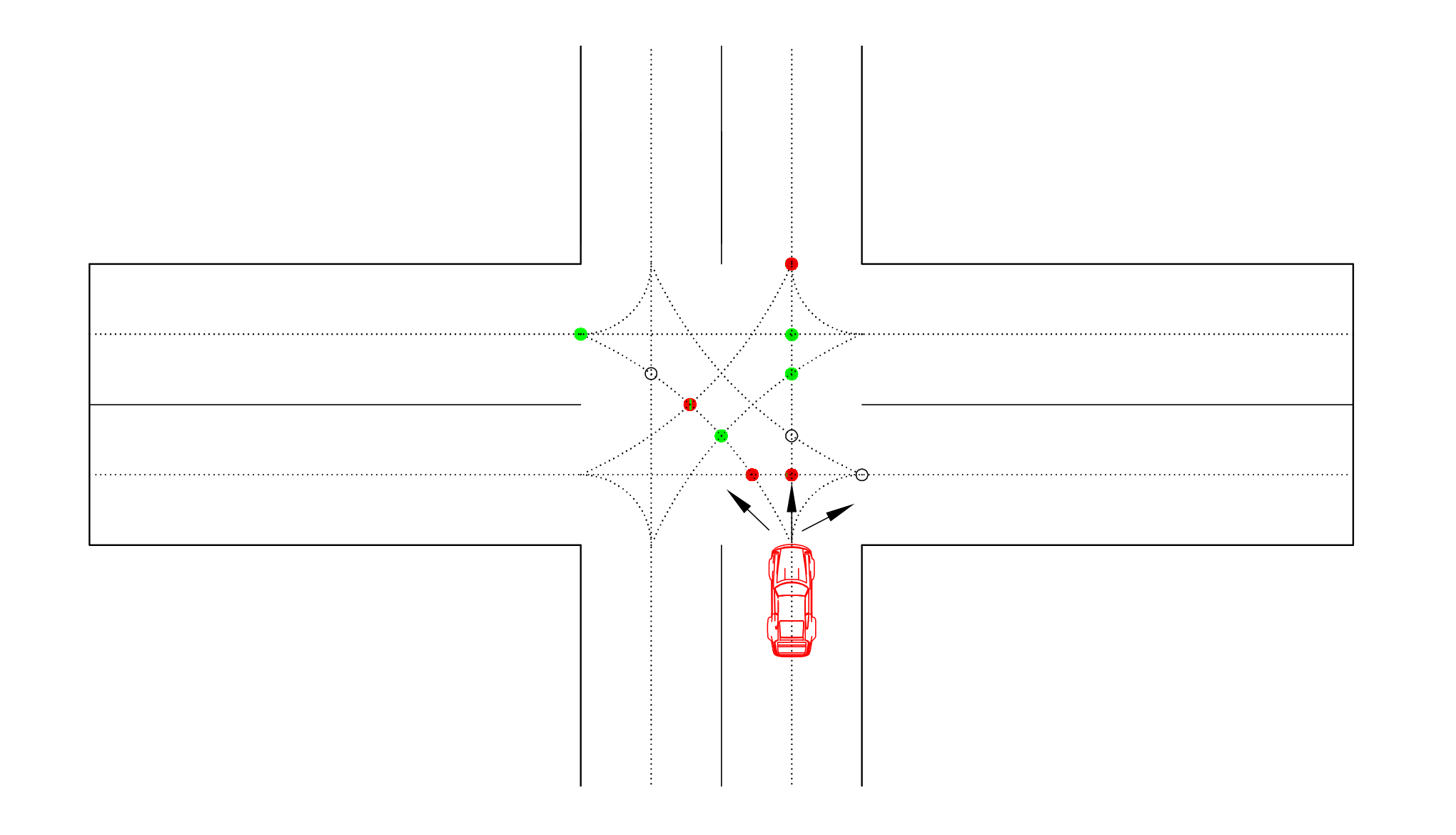
Remark (Framework Generalization). We can generalize the framework of any traffic scenario that involves multiple lanes leading to conflict zones beyond the merging configuration of Fig. 1. Suppose there are exit lanes and at most merging (conflict) points that a CAV may pass. Then, we can build FIFO queues for any such scenario, with any new arriving CAV assigned to the queues whose CAVs may have physical conflict with this new CAV. Then, according to the path that this CAV will choose, we can identify all the merging points that it may pass, and extend the FIFO queues with the proper order of passing merging points similar to Fig. 2. Note that the same merging point may appear at different columns in other rows (i.e., for other CAVs), so that the matching approach proposed in Sec. III-B should compare all other columns instead of just the same column as in the scenario of Fig. 1. The number of possible cases (excluding the case where is in the same lane as allthrough the CZ, as the case in Sec. III-B) is determined by where . The number of all possible cases with respect to the number of merging (conflict) points that a CAV may pass is given by . For example, a CAV in the intersection scenario shown in Fig. 3 may pass five merging points () (i.e., go straight or turn left) and there are four exit lanes . We have four FIFO queues, and extend them in the form of Table 2 by five MP columns. The number of possible cases is 56, but a CAV can easily find all the safe merging constraints (at most 5) that it needs to satisfy by looking up the extended queue similar to the form in Table 2.
IV SIMULATION RESULTS
All controllers in this section have been implemented using MATLAB and we have used the Vissim microscopic multi-model traffic flow simulation tool as a baseline for the purpose of making comparisons between our controllers and human-driven vehicles adopting standard car-following models used in Vissim. We used quadprog for solving QPs of the form (19) and ode45 to integrate the vehicle dynamics.
Referring to Fig. 1, CAVs arrive according to Poisson processes with rates 2000 CAVs per hour and 1200 CAVs per hour for the main and merging roads, respectively. The initial speed is also randomly generated with a uniform distribution over at the origins and , respectively. The parameters for (19) and (1) are: . We consider all class functions as cubic functions in (17) and consider uniformly distributed noise processes (in [-2, 2] for and in [-0.05, 0.05] for ) for all simulations.
| Method | Noise | Ave. time() | Ave. | Ave. obj. | |
|---|---|---|---|---|---|
| CBF | N/A | no | 14.7539 | 19.7241 | N/A |
| Vissim | N/A | 31.5351 | 17.0415 | 19.2993 | |
| OCBF | no | ||||
| yes | 22.7636 | 8.8133 | 10.4780 | ||
| Vissim | N/A | 31.5351 | 17.0415 | 73.4767 | |
| OCBF | no | ||||
| yes | 16.1811 | 11.2944 | 39.6146 | ||
| Vissim | N/A | 31.5351 | 17.0415 | 107.3404 | |
| OCBF | no | ||||
| yes | 14.4996 | 16.4412 | 54.5177 |
We compare the simulation results between Vissim (human driver), the CBF method [14] (by setting and in (19)) and the OCBF method, as shown in Table I. The CBF method is aggressive in travel time, and thus has larger energy consumption than both the OCBF method and human drivers. The OCBF method does better in both metrics than human drivers in Vissim, and achieves about 50% improvement in the objective function (7) under all three different trade-off parameters (recall that trades off travel time and energy in (6)).
In order to show whether the metrics have reached steady state or not, we present the history of average travel time and energy consumption in Figs. 4 and 5. The travel time in Vissim is still increasing, indicating that traffic congestion is becoming worse. However, both metrics in the CBF and OCBF methods are at steady state, providing evidence of their ability to better manage traffic congestion.


V CONCLUSIONS
We have shown how to transform a multi-lane merging problem into a decentralized optimal control problem, and combine OC with the CBF method to solve the merging problem for CAVs in order to deal with cases where the OC solution becomes difficult to obtain, as well as to handle the presence of noise in the vehicle dynamics by exploiting the ability of CBFs to add robustness to an OC controller. In addition, when considering more complex objective functions for which analytical optimal control solutions are unavailable, we can still adapt the CBF method to such objectives. Remaining challenges include research on resequencing and extensions to large traffic networks.
References
- [1] B. Schrank, B. Eisele, T. Lomax, and J. Bak. (2015) The 2015 urban mobility scorecard. Texas A&M Transportation Institute. [Online]. Available: http://mobility.tamu.edu
- [2] M. Tideman, M. van der Voort, B. van Arem, and F. Tillema, “A review of lateral driver support systems,” in Proc. IEEE Intelligent Transportation Systems Conference, pp. 992–999, Seatle, 2007.
- [3] D. D. Waard, C. Dijksterhuis, and K. A. Broohuis, “Merging into heavy motorway traffic by young and elderly drivers,” Accident Analysis and Prevention, vol. 41, no. 3, pp. 588–597, 2009.
- [4] P. Varaiya, “Smart cars on smart roads: problems of control,” IEEE Transactions on Automatic Control, vol. 38, no. 2, pp. 195–207, 1993.
- [5] M. Mukai, H. Natori, and M. Fujita, “Model predictive control with a mixed integer programming for merging path generation on motor way,” in Proc. IEEE Conference on Control Technology and Applications, pp. 2214–2219, Mauna Lani, 2017.
- [6] V. Milanes, J. Godoy, J. Villagra, and J. Perez, “Automated on-ramp merging system for congested traffic situations,” Trans. on Intelligent Transportation Systems, vol. 12, no. 2, pp. 500–508, 2011.
- [7] G. Domingues, J. Cabral, J. Mota, P. Pontes, Z. Kokkinogenis, and R. J. F. Rossetti, “Traffic simulation of lane-merging of autonomous vehicles in the context of platooning,” in IEEE International Smart Cities Conference, 2018, pp. 1–6.
- [8] W. Xiao and C. G. Cassandras, “Decentralized optimal merging control for connected and automated vehicles,” in Proc. of the American Control Conference, 2019, pp. 3315–3320.
- [9] ——, “Decentralized optimal merging control for connected and automated vehicles,” preprint arXiv:1809.07916, submitted to Automatica, 2018.
- [10] W. Cao, M. Mukai, and T. Kawabe, “Cooperative vehicle path generation during merging using model predictive control with real-time optimization,” Control Eng. Practice, vol. 34, pp. 98–105, 2015.
- [11] I. A. Ntousakis, I. K. Nikolos, and M. Papageorgiou, “Optimal vehicle trajectory planning in the context of cooperative merging on highways,” Transportation Research C, vol. 71, pp. 464–488, 2016.
- [12] A. D. Ames, S. Coogan, M. Egerstedt, G. Notomista, K. Sreenath, and P. Tabuada, “Control barrier functions: Theory and applications,” in Proc. of the European Control Conference, 2019, pp. 3420–3431.
- [13] W. Xiao and C. Belta, “Control barrier functions for systems with high relative degree,” in Proc. of 58th IEEE Conference on Decision and Control, Nice, France, 2019, pp. 474–479.
- [14] W. Xiao, C. Belta, and C. G. Cassandras, “Decentralized merging control in traffic networks: A control barrier function approach,” in Proc. ACM/IEEE International Conference on Cyber-Physical Systems, Montreal, Canada, 2019, pp. 270–279.
- [15] W. Xiao, C. G. Cassandras, and C. Belta, “Decentralized merging control in traffic networks with noisy vehicle dynamics: A joint optimal control and barrier function approach,” in Proc. IEEE 22nd Intelligent Transportation Systems Conference, 2019, pp. 3162–3167.
- [16] Y. J. Zhang and C. G. Cassandras, “A decentralized optimal control framework for connected automated vehicles at urban intersections with dynamic resequencing,” in Proc. 57th IEEE Conference on Decision and Control, pp. 217–222, Miami, 2018.
- [17] H. Xu, Y. Zhang, L. Li, and W. Li, “Cooperative driving at unsignalized intersections using tree search,” preprint arXiv:1902.01024, 2019.
- [18] W. Xiao and C. G. Cassandras, “Decentralized optimal merging control for connected and automated vehicles with optimal dynamic resequencing,” in Proc. of the American Control Conference, 2020, to appear.
- [19] K. Vogel, “A comparison of headway and time to collision as safety indicators,” Accident Analysis & Prevention, vol. 35, no. 3, pp. 427–433, 2003.
- [20] H. K. Khalil, Nonlinear Systems. Prentice Hall, 3rd edition, 2002.