Hubble Sinks In The Low-Redshift Swampland
Abstract
Local determinations of the Hubble constant favour a higher value than Planck based on CMB and CDM. Through a model-independent expansion, we show that low redshift () data comprising baryon acoustic oscillations (BAO), cosmic chronometers and Type Ia supernovae has a preference for Quintessence models that lower relative to CDM. In addition, we confirm that an exponential coupling to dark matter cannot alter this conclusion in the same redshift range. Our results leave open the possibility that a coupling in the matter-dominated epoch, potentially even in the dark ages, may yet save from sinking in the string theory Swampland.
I Introduction
Last century Allan Sandage framed cosmology as the search for two numbers Sandage. 50 years later, it is widely accepted that the deceleration parameter is negative Riess:1998cb; Perlmutter:1998np, and the Hubble constant is known to within Aghanim:2018eyx; Riess:2019cxk; Wong:2019kwg; Freedman:2019jwv; Pesce:2020xfe, making it one of the best measured quantities in late-time cosmology. At the lower end of this window, one finds the Planck determination based on the cosmological model CDM and the Cosmic Microwave Background (CMB) Aghanim:2018eyx. In contradistinction, a host of local determinations favour higher values Riess:2019cxk; Wong:2019kwg; Freedman:2019jwv; Pesce:2020xfe, resulting in Hubble tension Verde:2019ivm, an intriguing discrepancy between early and late Universe determinations of .
The convergence of different experiments suggests that a high local is legit (to lose one experiment, may be regarded as a misfortune; to lose all looks like carelessness). One logical possibility, advocated by the Swampland programme within string theory Agrawal:2018own is that we replace with Quintessence Copeland:2006wr; Tsujikawa:2013fta, the simplest alternative in effective field theory (EFT). Against this backdrop, our goal is to ascertain if is raised or lowered relative to CDM by the Swampland.
To date the Swampland Vafa:2005ui has led to an intriguing web of conjectures (see Brennan:2017rbf; Palti:2019pca for reviews), which remarkably impinge on the real world. The most consequential precludes de Sitter vacua Obied:2018sgi and is in conflict with CDM Agrawal:2018own. Subsequent to-and-fro discussion led to a refinement Garg:2018reu; Ooguri:2018wrx (also Andriot:2018wzk), thus allowing the conjecture to co-exist with the Higgs’ potential Denef:2018etk. Nevertheless, the de Sitter conjecture is constrained by cosmological data Heisenberg:2018yae; Akrami:2018ylq; Raveri:2018ddi and it was highlighted early on that Hubble tension may be an issue Colgain:2018wgk.
Here, we return to the Hubble tension thread within the context of generic Quintessence models Copeland:2006wr; Tsujikawa:2013fta. Recall that “Quintessence” may be defined as a canonically coupled scalar with scalar potential and an equation of state (EoS) for dark energy that is bounded below . However, the latter can be relaxed within EFT by coupling dark matter to dark energy through “coupled Quintessence” Wetterich:1994bg; Amendola:1999er; Das:2005yj. While it is known that a coupling allows one to effectively reduce and hence to raise DiValentino:2016hlg; DiValentino:2019jae, in contrast, specific uncoupled Quintessence models lower Vagnozzi:2019ezj; Alestas:2020mvb; Vagnozzi:2018jhn; Colgain:2019joh (see also Table I Agrawal:2019dlm) 11 1 The CPL model Chevallier:2000qy; Linder:2002et clearly works well as a model-independent approach to dark energy when confronting observations. However, since the equation of state is a quantity derived from a potential, the fact that the CPL expansion is truncated at linear order in means that the corresponding potential will be constrained. It is not a generic Quintessence model, especially when one fits data from CMB . In particular, the Quintessence potential , does not admit a CPL prescription., thus implying that is in the Swampland. In this letter we show that this is more generally true.
In contrast to models with fixed potentials, e. g. vandeBruck:2017idm; vandeBruck:2019vzd; Miranda:2017rdk; Gomez-Valent:2020mqn; Ruchika:2020avj, here we exploit perturbation at low redshift to work in a model-independent way. In short, we construct a large class of “bottom-up” potentials, which we confront with direct measurements of the Hubble parameter inferred from cosmic chronometers CC1; CC2; CC3; CC4; CC5; CC6; CC7 and BAO Alam:2016hwk 22 2 Concretely, our Taylor expansion has only enough parameters to approximate the angular diameter distance data to , so we can only use the data and its covariance matrix. This is not a problem for the isotropic BAO at and .. In addition, we include low- BAO measurements by 6dF Beutler:2011hx () and SDSS-MGS surveys Ross:2014qpa (), and determinations of from type Ia supernovae Riess:2017lxs (derived from Scolnic:2017caz). Finally, we allow for an exponential potential, which is the dark matter-Quintessence coupling of choice in string theory.
Our findings are simply expressed. Quintessence models prefer a lower value than CDM. Moreover, neither a prior Riess:2019cxk nor an exponential coupling to dark matter - provided it is constrained by galaxy warps Desmond:2018euk; Desmond:2018sdy - can change the conclusion in the redshift range. Models where the coupling is turned on earlier are still viable, but only at higher redshifts, namely within the matter-dominated era (). Furthermore, if the coupling is turned on in the dark ages beyond Agrawal:2019dlm, a proper test of such a scenario may rest upon future developments in 21-cm cosmology Pritchard:2011xb; Bowman:2018yin. Nevertheless, this loophole aside, low-redshift observations place the de Sitter conjecture Obied:2018sgi at odds with local determinations of , since the class of models championed by the conjecture only exacerbates Hubble tension.
II Set-up
We consider flat FLRW spacetime and the following coupled Quintessence equations:
| (1) | |||||
| (2) |
where dots denote time derivatives, is the scale factor and is the Hubble parameter. In addition, is a coupling between the dark matter density and the Quintessence field , while denotes the baryonic matter density. Observe that setting , we recover uncoupled Quintessence with matter density . These equations allow an effective EoS when Das:2005yj. Concretely, we consider where and are constant. Finally, observe that we have set for simplicity.
We emphasise that the basic ingredients of equations (1) and (2), i. e. a canonically coupled scalar, a potential and an exponential coupling are ubiquitous in low-energy effective descriptions of string theory, e. g. Brax:1999gp; Anchordoqui:2019amx; Anchordoqui:2020sqo; Chiang:2018jdg; DiValentino:2019exe; Ferrara:2019tmu; Montefalcone:2020vlu, thus, the basic building blocks of the Swampland are in place. Now, to solve these equations, we recall the usual definition of the scale factor in terms of redshift , normalised so that today. Using the chain rule, one establishes that , and it is easy to recast the Friedmann (1) and scalar equation (2) in terms of redshift. We consider the following expansion for the scalar,
| (3) |
around its value today at , where and are constants. At small , is small, and we can further expand the potential:
| (4) |
where we have defined , etc. The Hubble parameter to third order in redshift is
| (5) |
where may be expressed in terms of the parameters as,
| (6) | |||||
Evidently, when , we recover the CDM cosmology, while at , we have . Observe that we have employed the usual definitions , to define the baryonic and dark matter density today.
Note that is our reference model. Since we are working perturbatively around , we first establish the range of validity of the expansion. To see this, we note that when , namely the canonical Planck value Aghanim:2018eyx, the corresponding values for are . Concretely, if we demand that our expansion is within of the exact analytic result, , then the linear, quadratic and cubic approximations are good to and , respectively.
The potential and its derivatives at can be expressed in terms of :
| (7) | |||||
| (8) | |||||
| (9) | |||||
where for a given coupling , we have a one-to-one correspondence between and . Note also that is the dark energy density today . The effective EoS can easily be worked out,
| (10) | |||||
Interestingly, regardless of the value of , at and a crossing into the phantom regime () happens only at higher redshift. Note that when , we simply denote as .
III Methodology
We begin by generating triples , in a normal distribution about with a uniform standard deviation, which we take to be 33 3 Increasing this value or adopting a uniform distribution does not change our results.. We impose a conservative redshift cut-off, , and impose
| (11) |
to ensure perturbation makes sense, i. e. higher order numbers are smaller. Note that these cuts can be implemented without establishing a best-fit value of and we are not imposing slow-roll.

For the triples surviving these primary cuts, we perform two-parameter fits of the data CC1; CC2; CC3; CC4; CC5; CC6; CC7; Alam:2016hwk; Beutler:2011hx; Ross:2014qpa; Riess:2017lxs 44 4 For isotropic BAO, the expansion suffices. and demand that
| (12) |
once again to ensure a valid expansion. In addition, we impose the nominal restriction , which is in line with weak lensing results Abbott:2018xao; Joudaki:2019pmv, and impose the constraints from FIG. 1, which we have inferred from a Markov Chain Monte Carlo (MCMC) exploration of cosmic chronometer, BAO and Pantheon data below . Observe that in contrast to Heisenberg:2018yae, our bounds come from low redshift data, which means they are less constraining, and for uncoupled models, we impose .
It is worth emphasising that our expansion is expected to be valid to , but if we include distance moduli or angular diameter distance measurements, since they are integrated quantities, the approximation holds only for . This allows us to easily accommodate isotropic BAO at Beutler:2011hx and Ross:2014qpa, but for higher redshift BAO we are restricted to and its covariance matrix. For this reason, there is extra information in FIG 1. and this leads to additional constraints. Finally, since we have a large parameter space, e.g. , one can expect any best-fit values to be within of CDM, which ultimately favours the standard model. However, since our interest here is exploring the effect on of changing the underlying potential (theory), we simply scan over and .
Once the cuts are imposed, we are left with a large class of “bottom-up” Quintessence models, which we further divide into cosmologies where increases/decreases relative to the CDM model, i. e. . For reference, we record the best-fit values in this case,
| (13) |
Note that the values are pretty consistent with Planck Aghanim:2018eyx and due to our inflated errors, this represents a discrepancy with the highest local determination based on cepheid-calibrated supernovae Riess:2019cxk.
Once the coupling is introduced, the dark matter particles are subject to a long-range attractive force with an effective Newton’s constant . While the CMB constrains the conformal coupling to be vandeBruck:2017idm; Miranda:2017rdk, if the coupling is turned on at late-times, e.g. Agrawal:2019dlm, this constraint can be evaded. Nevertheless, stronger constraints exist for galaxies up to redshift Desmond:2018euk; Desmond:2018sdy, whereby . This number will be constrained further in future, but here we settle on the value . This relaxes the constraint of Desmond:2018euk; Desmond:2018sdy slightly, but still preserves its integrity as a strong observational bound. Finally, since baryonic matter is uncoupled, we instead adopt the Planck prior and only fit and .

IV Results
In FIG. 2 we present a plot of the as a function of the best-fit for uncoupled models, where a dashed line denotes the for the CDM model, . From the plot it is clear that deviations from CDM that lower are favoured by the data. In contrast, may increase, but this worsens the fit to the data. Interestingly, we find no exceptions to this statement in 87,675 random models and we have checked that adding a prior Riess:2019cxk throughout does not change our conclusions.

In FIG. 3 we present the same plot but for coupled Quintessence models with . We are again making a comparison to the CDM model. Concretely, here we first identified triples of , i. e. potentials where , thus ensuring that the uncoupled model is a bona fide Quintessence model, before adding the coupling. Once the coupling is added, we can enter the region of parameter space and we repeat the fitting procedure. Thus, the configurations presented in FIG. 3 are a subset of the FIG. 2 configurations, but subject to a coupling. In contrast to the uncoupled case, the range of is extended, but since is small, the effect is not so great. One could choose a larger coupling, but this would bring us into conflict with Desmond:2018euk; Desmond:2018sdy. Finally, we have checked that removing the poorer quality cosmic chronometer data does not change our conclusions.
Finally, we can make some remarks on the universal constants from the de Sitter Conjecture Obied:2018sgi; Garg:2018reu; Ooguri:2018wrx. We find that models that lower occur at smaller values of relative to models that raise . Ostensibly, this means that the de Sitter conjecture may (theoretically) favour models that raise . That being said, such models have exclusively , whereas models that lower allow . For this reason, the Refined de Sitter Conjecture Garg:2018reu; Ooguri:2018wrx favours models with lower than CDM. Note, this is a statement that does not rely on , but still makes use of fits to data.
V Discussion
With an eye on the de Sitter Swampland conjecture Obied:2018sgi, we have performed a scan over (coupled) Quintessence models at low redshift. Since are in one-to-one correspondence with , our best-fit values for probe different models (potentials) in the vicinity of CDM. Within our assumptions and the data employed we arrive at the conclusion that decreases relative to CDM in any Quintessence model with an exponential coupling. Such models are expected to arise from string theory constructions, e. g. Anchordoqui:2019amx; Anchordoqui:2020sqo, but explicit constructions are especially challenging Cicoli:2018kdo; Hebecker:2019csg.
Our analysis here employs Taylor expansion around , so we are simply assuming analyticity. This allows us to describe a large class of single field Quintessence models with a canonically normalised kinetic term. Nevertheless, to turn any of these models into viable cosmologies, one needs to ensure that there exists a high redshift completion to CMB. In fact, modulo the fact that truncating the CDM or CPL model Chevallier:2000qy; Linder:2002et at linear order in is guaranteed to constrain the potential (see comments in the appendix) 55 5 Also note that CPL is a linear model and does not allow wiggles in the EoS, whereas coupled Quintessence models do., the results of Vagnozzi:2018jhn suggest little will change for uncoupled Quintessence models that admit a high redshift completion to CMB. So, uncoupled Quintessence is clearly at odds with high local determinations of Riess:2019cxk; Wong:2019kwg; Freedman:2019jwv; Pesce:2020xfe. In short, if Hubble tension in CDM is now a “problem” or “crisis”, Quintessence simply instills a sense of panic.
This leaves a coupling between Quintessence and dark matter as a potential loophole. Here we have focused on the exponential coupling, which is the most natural from string theory, and imposed strict bounds that are derived from the absence of differential fifth forces in galaxy warps Desmond:2018euk; Desmond:2018sdy. We find that the coupling is too small to induce any effect within the redshift range. Indeed, it is clear from equation (II) that the term in the Hubble parameter is unaffected by the coupling, so the coupling is suppressed near . With such a small coupling, any interaction between Quintessence and dark matter will have to act over an extended redshift range, in other words beyond the dark energy-dominated regime, to make progress on Hubble tension. In particular, we may have to embrace a coupling that acts in the dark ages Agrawal:2019dlm, which is currently beyond the scope of experiment, but interestingly, this may quickly change Bowman:2018yin.
Acknowledgements
We thank S. Angus, S. Appleby, H. Desmond, A. Hebecker, C. Krishnan, A. A. Sen, P. Steinhardt, S. Vagnozzi, C. van de Bruck and J. Zhang for correspondence and discussion. This work was supported in part by the Korea Ministry of Science, ICT & Future Planning, Gyeongsangbuk-do and Pohang City. LH is supported by funding from the European Research Council (ERC) under the European Unions Horizon 2020 research and innovation programme grant agreement No 801781 and by the Swiss National Science Foundation grant 179740. MMShJ would like to thank the hospitality of ICTP HECAP where this research carried out. MMShJ acknowledges the support by INSF grant No 950124 and Saramadan grant No. ISEF/M/98204.
Appendix A Comment on CPL model
In this section, we review the analysis of Scherrer Scherrer:2015tra, before taking it further using a combination of CMB, BAO and SNe data. Recall that the CPL model Chevallier:2000qy; Linder:2002et can be expected to correspond to a specific class of potentials when Scherrer:2015tra. More concretely, one can solve the potential in terms of the scale factor Scherrer:2015tra,
| (14) |
where we have normalised the potential so that . Now, to determine as a function of , one just needs to perform the following integral:
| (15) |
where following Scherrer:2015tra, we adopt . Note that is only defined up to a constant, but to fix it we assume . As can be seen from FIG. 1 or FIG. 2 of Scherrer:2015tra, CPL models are not generic and they correspond to a specific class of Quintessence models.
Here, we will take the observation a little further in light of the results of Vagnozzi et al. Vagnozzi:2018jhn. There, given that they are fitting CMB data at , the authors impose the conditions,
| (16) |
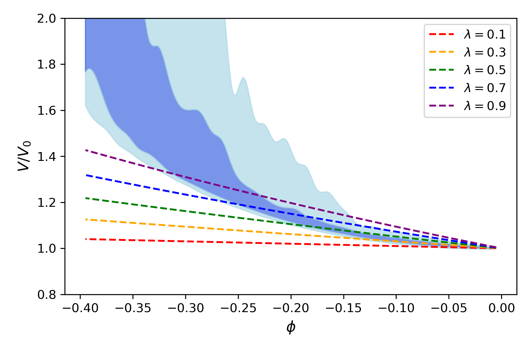
which will guarantee that for all . So, here we will take the CMB+BAO+Pantheon MCMC chains from Planck analysis of the CPL model Aghanim:2018eyx and impose the constraints (16). This then leaves one with 400 odd pairs of , which given the preference of the data for the cosmological constant are all pretty close to . We next integrate (15) from to (). This provides us a mapping between and for each CPL model, i. e. each pair. One can then work outwards from , corresponding to , to determine as a function of . In practice, we bin into bins of and extract out the mean and , intervals in each bin, before applying a spline to these values. The end result is shown in FIG. 4.
There are a number of take-homes from the plot. First, for reasons that we have explained above, the Quintessence potential corresponding to the CPL model is pretty constrained. This is even more apparent when one integrates (15) all the way to . This is in line with earlier comments in ref. Scherrer:2015tra. Secondly, CMB+BAO+Pantheon data has a clear preference for the cosmological constant , so it is no surprise that the potential is extremely flat as one approaches (). Finally, it is worth noting that if one interprets this even in terms of the simplest Quintessence model, one may come to the erroneous conclusion that they are ruled out. This is not the case, it is just simply that the Quintessence potentials corresponding to the CPL model are indeed very special, so special that falls outside the class for certain ranges of , or the corresponding ranges in . That being said, it should be easy to show that our results are consistent with Heisenberg:2018yae in the small regime, i. e. at late times.
References
- (1) Physics Today 23, 2, 34 (1970)
- (2) A. G. Riess et al. [Supernova Search Team], Astron. J. 116, 1009 (1998) [astro-ph/9805201].
- (3) S. Perlmutter et al. [Supernova Cosmology Project Collaboration], Astrophys. J. 517, 565 (1999) [astro-ph/9812133].
- (4) N. Aghanim et al. [Planck], [arXiv:1807.06209 [astro-ph.CO]].
- (5) A. G. Riess, S. Casertano, W. Yuan, L. M. Macri and D. Scolnic, Astrophys. J. 876 (2019) no.1, 85 [arXiv:1903.07603 [astro-ph.CO]].
- (6) K. C. Wong et al., [arXiv:1907.04869 [astro-ph.CO]].
- (7) W. L. Freedman, B. F. Madore, D. Hatt, T. J. Hoyt, I. Jang, R. L. Beaton, C. R. Burns, M. G. Lee, A. J. Monson, J. R. Neeley, M. M. Phillips, J. A. Rich and M. Seibert, [arXiv:1907.05922 [astro-ph.CO]].
- (8) D. Pesce, J. Braatz, M. Reid, A. Riess, D. Scolnic, J. Condon, F. Gao, C. Henkel, C. Impellizzeri, C. Kuo and K. Lo, Astrophys. J. 891 (2020) no.1, L1 [arXiv:2001.09213 [astro-ph.CO]].
- (9) L. Verde, T. Treu and A. Riess, [arXiv:1907.10625 [astro-ph.CO]].
- (10) P. Agrawal, G. Obied, P. J. Steinhardt and C. Vafa, Phys. Lett. B 784 (2018), 271-276 [arXiv:1806.09718 [hep-th]].
- (11) E. J. Copeland, M. Sami and S. Tsujikawa, Int. J. Mod. Phys. D 15, 1753 (2006) [hep-th/0603057].
- (12) S. Tsujikawa, Class. Quant. Grav. 30, 214003 (2013) [arXiv:1304.1961 [gr-qc]].
- (13) C. Vafa, [arXiv:hep-th/0509212 [hep-th]].
- (14) T. D. Brennan, F. Carta and C. Vafa, PoS TASI2017 (2017), 015 [arXiv:1711.00864 [hep-th]].
- (15) E. Palti, Fortsch. Phys. 67 (2019) no.6, 1900037 [arXiv:1903.06239 [hep-th]].
- (16) G. Obied, H. Ooguri, L. Spodyneiko and C. Vafa, [arXiv:1806.08362 [hep-th]].
- (17) H. Ooguri, E. Palti, G. Shiu and C. Vafa, Phys. Lett. B 788, 180 (2019) [arXiv:1810.05506 [hep-th]].
- (18) S. K. Garg and C. Krishnan, arXiv:1807.05193 [hep-th].
- (19) D. Andriot, Phys. Lett. B 785 (2018), 570-573 [arXiv:1806.10999 [hep-th]].
- (20) F. Denef, A. Hebecker and T. Wrase, Phys. Rev. D 98 (2018) no.8, 086004 [arXiv:1807.06581 [hep-th]].
- (21) L. Heisenberg, M. Bartelmann, R. Brandenberger and A. Refregier, Phys. Rev. D 98, no. 12, 123502 (2018) [arXiv:1808.02877 [astro-ph.CO]].
- (22) Y. Akrami, R. Kallosh, A. Linde and V. Vardanyan, Fortsch. Phys. 67, no. 1-2, 1800075 (2019) [arXiv:1808.09440 [hep-th]].
- (23) M. Raveri, W. Hu and S. Sethi, Phys. Rev. D 99, no. 8, 083518 (2019) [arXiv:1812.10448 [hep-th]].
- (24) E. Ó Colgáin, M. H. van Putten and H. Yavartanoo, Phys. Lett. B 793 (2019), 126-129 [arXiv:1807.07451 [hep-th]].
- (25) C. Wetterich, Astron. Astrophys. 301 (1995), 321-328 [arXiv:hep-th/9408025 [hep-th]].
- (26) L. Amendola, Phys. Rev. D 62, 043511 (2000) [astro-ph/9908023].
- (27) S. Das, P. S. Corasaniti and J. Khoury, Phys. Rev. D 73, 083509 (2006) [astro-ph/0510628].
- (28) E. Di Valentino, A. Melchiorri and J. Silk, Phys. Lett. B 761 (2016), 242-246 [arXiv:1606.00634 [astro-ph.CO]].
- (29) E. Di Valentino, A. Melchiorri, O. Mena and S. Vagnozzi, Phys. Rev. D 101 (2020) no.6, 063502 [arXiv:1910.09853 [astro-ph.CO]].
- (30) S. Vagnozzi, [arXiv:1907.07569 [astro-ph.CO]].
- (31) G. Alestas, L. Kazantzidis and L. Perivolaropoulos, [arXiv:2004.08363 [astro-ph.CO]].
- (32) S. Vagnozzi, S. Dhawan, M. Gerbino, K. Freese, A. Goobar and O. Mena, Phys. Rev. D 98 (2018) no.8, 083501 [arXiv:1801.08553 [astro-ph.CO]].
- (33) E. Ó Colgáin and H. Yavartanoo, Phys. Lett. B 797 (2019), 134907 [arXiv:1905.02555 [astro-ph.CO]].
- (34) P. Agrawal, G. Obied and C. Vafa, arXiv:1906.08261 [astro-ph.CO].
- (35) M. Chevallier and D. Polarski, Int. J. Mod. Phys. D 10, 213 (2001) [gr-qc/0009008].
- (36) E. V. Linder, Phys. Rev. Lett. 90, 091301 (2003)
- (37) C. Van De Bruck and J. Mifsud, Phys. Rev. D 97, no. 2, 023506 (2018) [arXiv:1709.04882 [astro-ph.CO]].
- (38) C. van de Bruck and C. C. Thomas, Phys. Rev. D 100, no. 2, 023515 (2019) [arXiv:1904.07082 [hep-th]].
- (39) V. Miranda, M. Carrillo González, E. Krause and M. Trodden, Phys. Rev. D 97 (2018) no.6, 063511 [arXiv:1707.05694 [astro-ph.CO]].
- (40) A. Gómez-Valent, V. Pettorino and L. Amendola, [arXiv:2004.00610 [astro-ph.CO]].
- (41) Ruchika, K. Dutta, A. Mukherjee and A. A. Sen, [arXiv:2005.08813 [astro-ph.CO]].
- (42) C. Zhang, H. Zhang, S. Yuan, T-J. Zhang and Y-C. Sun, Res. Astron. Astrophys. 14 (2014) 1221 [arXiv:1207.4541]
- (43) R. Jiménez, L. Verde, T. Treu and D. Stern, Astrophys. J. 593 (2003) 622 [arXiv:astro-ph/0302560]
- (44) J. Simon, L. Verde and R. Jiménez, Phys. Rev. D71 (2005) 123001 [arXiv:astro-ph/0412269]
- (45) M. Moresco et al., J. Cosmol. Astropart. Phys. 1208 (2012) 006 [arXiv:1201.3609]
- (46) M. Moresco et al., J. Cosmol. Astropart. Phys. 1605 (2016) 014 [arXiv:1601.01701]
- (47) A.L. Ratsimbazafy et al., Mon. Not. Roy. Astron. Soc. 467 (2017) 3239 [arXiv:1702.00418]
- (48) D. Stern, R. Jiménez, L. Verde, M. Kamionkowski and S.A. Stanford, J. Cosmol. Astropart. Phys. 1002 (2010) 008 [arXiv:0907.3149]
- (49) S. Alam et al. [BOSS], Mon. Not. Roy. Astron. Soc. 470, no.3, 2617-2652 (2017) [arXiv:1607.03155 [astro-ph.CO]].
- (50) F. Beutler, C. Blake, M. Colless, D. Jones, L. Staveley-Smith, L. Campbell, Q. Parker, W. Saunders and F. Watson, Mon. Not. Roy. Astron. Soc. 416 (2011), 3017-3032 [arXiv:1106.3366 [astro-ph.CO]].
- (51) A. J. Ross, L. Samushia, C. Howlett, W. J. Percival, A. Burden and M. Manera, Mon. Not. Roy. Astron. Soc. 449 (2015) no.1, 835-847 [arXiv:1409.3242 [astro-ph.CO]].
- (52) A. G. Riess et al., Astrophys. J. 853 (2018) no.2, 126 [arXiv:1710.00844 [astro-ph.CO]].
- (53) D. Scolnic et al., Astrophys. J. 859 (2018) no.2, 101 [arXiv:1710.00845 [astro-ph.CO]].
- (54) H. Desmond, P. G. Ferreira, G. Lavaux and J. Jasche, Mon. Not. Roy. Astron. Soc. 483 (2019) no.1, L64-L68 [arXiv:1802.07206 [astro-ph.CO]].
- (55) H. Desmond, P. G. Ferreira, G. Lavaux and J. Jasche, Phys. Rev. D 98 (2018) no.6, 064015 [arXiv:1807.01482 [astro-ph.CO]].
- (56) J. R. Pritchard and A. Loeb, Rept. Prog. Phys. 75 (2012), 086901 [arXiv:1109.6012 [astro-ph.CO]].
- (57) J. D. Bowman, A. E. E. Rogers, R. A. Monsalve, T. J. Mozdzen and N. Mahesh, Nature 555 (2018) no.7694, 67-70 [arXiv:1810.05912 [astro-ph.CO]].
- (58) P. Brax and J. Martin, Phys. Lett. B 468 (1999), 40-45 [arXiv:astro-ph/9905040 [astro-ph]].
- (59) C. Chiang and H. Murayama, [arXiv:1808.02279 [hep-th]].
- (60) L. A. Anchordoqui, I. Antoniadis, D. Lï¿œst, J. F. Soriano and T. R. Taylor, arXiv:1912.00242 [hep-th].
- (61) L. A. Anchordoqui, I. Antoniadis, D. Lust and J. F. Soriano, [arXiv:2005.10075 [hep-th]].
- (62) S. Ferrara, M. Tournoy and A. Van Proeyen, Fortsch. Phys. 68 (2020) no.2, 1900107 [arXiv:1912.06626 [hep-th]].
- (63) E. Di Valentino, R. Z. Ferreira, L. Visinelli and U. Danielsson, Phys. Dark Univ. 26 (2019), 100385 [arXiv:1906.11255 [astro-ph.CO]].
- (64) G. Montefalcone, P. J. Steinhardt and D. H. Wesley, [arXiv:2005.01143 [hep-th]].
- (65) T. Abbott et al. [DES], Phys. Rev. D 99 (2019) no.12, 123505 [arXiv:1810.02499 [astro-ph.CO]].
- (66) S. Joudaki et al. [arXiv:1906.09262 [astro-ph.CO]].
- (67) M. Cicoli, S. De Alwis, A. Maharana, F. Muia and F. Quevedo, “De Sitter vs Quintessence in String Theory,” Fortsch. Phys. 67 (2019) no.1-2, 1800079 [arXiv:1808.08967 [hep-th]].
- (68) A. Hebecker, T. Skrzypek and M. Wittner, JHEP 11 (2019), 134 [arXiv:1909.08625 [hep-th]].
- (69) R. J. Scherrer, Phys. Rev. D 92 (2015) no.4, 043001 [arXiv:1505.05781 [astro-ph.CO]].