Complex Sequential Understanding through the Awareness of Spatial and Temporal Concepts
Abstract
Understanding sequential information is a fundamental task for artificial intelligence. Current neural networks attempt to learn spatial and temporal information as a whole, limited their abilities to represent large scale spatial representations over long-range sequences. Here, we introduce a new modeling strategy called Semi-Coupled Structure (SCS), which consists of deep neural networks that decouple the complex spatial and temporal concepts learning. Semi-Coupled Structure can learn to implicitly separate input information into independent parts and process these parts respectively. Experiments demonstrate that a Semi-Coupled Structure can successfully annotate the outline of an object in images sequentially and perform video action recognition. For sequence-to-sequence problems, a Semi-Coupled Structure can predict future meteorological radar echo images based on observed images. Taken together, our results demonstrate that a Semi-Coupled Structure has the capacity to improve the performance of LSTM-like models on large scale sequential tasks.
Complex sequential tasks involve extremely high-dimensional spatial signal over long timescales. Neural networks have made breakthroughs in sequential learning graves2013generating; sutskever2014sequence, visual understanding krizhevsky2012imagenet; he2016deep; he2017mask, and robotic tasks levine2016end; schulman2015trust. Conventional neural networks treat spatial and temporal information as a whole, processing these parts together. This limits their ability to solve complex sequential tasks involving high-dimensional spatial and temporal components feichtenhofer2018slowfast; kim2017residual. A natural idea to address this limitation is to learn the two different concepts relatively independently.
Here, we introduce a structure that decouples spatial and temporal information, implicitly learning respective spatial and temporal concepts through a deep comprehensive model. We find that such concept decomposition significantly simplifies the learning and understanding process of complex sequences. Due to the differentiable property of this structure, which we call Semi Coupled Structure (SCS), we can train it end to end with gradient descent, allowing it to effectively learn to decouple and integrate information in a goal-directed manner.

1 Awareness of Spatial and Temporal Concept
In the brain, there are two different pathways that feed temporal information and contextual representations respectively into the hippocampus kitamura2015entorhinal. This implies that spatial and temporal concepts are learnt by different cognitive mechanisms and, moreover, that they should be synchronized in order to effectively process sequential information. Taking inspiration from this mechanism in the brain, the deep neural model that is implicitly aware of the two concepts can be formulated as:
| (1) |
where is the input, and and are the parameters to optimize. aims at extracting spatial information, while is designed to handle temporal learning. These two kinds of information are fed into which is designed to output the final processing results, just like the hippocampus.
We further advance our model by considering the fact that spatial and temporal information are deeply coupled with each other, when processed by a brain oliveri2009spatial. Therefore, the model can naturally be extended as a deep nested structure to model such mutual-coupling. We define the coupling unit as:
| (2) |
thus, the deep spatial-temporal Semi-Coupled Structure can be expressed as:
| (3) |
where is the depth of the deep nested model, and and are the parameter sets.
In this structure, spatial and temporal information are intertwined deeply and collaboratively, meanwhile, and are responsible for spatial and temporal concept processing respectively. To this end, we propose two design paradigms (see Fig. 1).
- •
Structure Paradigms and work as their roles by their different structural designs. At a certain time stamp of the sequence, the structure of should have access to the temporal information of other stamps in the sequence like the Recurrent Neural Network (RNN). While for , it has no direct connection to the samples of other time stamps, so it can focus on the spatial information, which normally can be a CNN structure.
- •
Task Paradigms Because of the deep nested structure, and will disturb each other. To make and further focus on their roles, besides the main goal: , we assign two extra sub-goals: and , where and share the same model components and parameters with . We also call and as the spatial and temporal indicating goals which can reflect the qualities of spatial and temporal features. The key design is to make both two indicating goals only impact on their own parameters: or . That is, in , and in , . The specific definition of the sub-goals depends on different tasks. Taking action recognition as an example, can be human poses in a single frame that is unrelated to temporal information but useful for action understanding, and can be the estimates of optical flow.
This new modeling strategy is called Semi-Coupled Structure (SCS). It is a general framework that is easy to be revised to fit various applications. If the temporal indicating label of a specific application is difficult to provide, we find that only is enough to encourage to focus on spatial learning, and can naturally take the responsibility of the remain (temporal) information.
Discussion
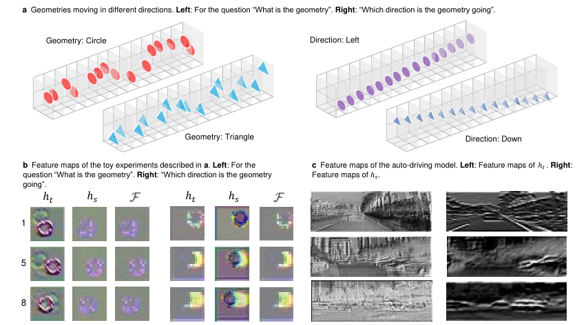
The proposed SCS makes each component be responsible for a specific sub-concept (spatial or temporal). This strategy widely exists in the brain using several different encephalic regions to complete a single complex task wolman2012tale; diez2015novel. During this process, our method learns to separate temporal and spatial information, even though we do not define them separately. There are previous works that also try to separate the temporal and spatial information, but they adopt the hand-craft spatial and temporal definitions, like Two-Stream model simonyan2014two which uses optical flow lucas1986generalized to define temporal information and SlowFast Networks feichtenhofer2018slowfast that uses asymmetrical spatial and temporal sampling density to distinguish and define them. Fig. 2 illustrates that SCS can successfully decouple the temporal and spatial information in visual sequences. In a toy experiment, the visual sequences show different geometries moving in different directions (see Fig. 2 a for details) and we note that our method outperforms LSTM hochreiter1997long on recognizing “Which direction is the geometry going?” when it encounters a specific geometry it never saw and “what is the geometry?” when the motion is disordered. Fig. 2 b shows the feature maps of and , and we can primarily recognize that represents temporal-related features and is for the spatial one from the viewpoint of human vision. Interestingly, our model can quantitatively indicate how important the temporal information is toward the final goal by comparing the indicating goals and , thanks to the awareness of the temporal and spatial concepts. We believe this quantitative indicator will largely benefit the sequential analysis.
2 Performance Profiling on Academic and Reality Datasets
2.1 Video action recognition experiments
To investigate the capacity of the Semi-Coupled Structure, we conduct the first experiment on video action recognition task. We choose UCF-101 soomro2012ucf101, HMDB-51 kuehne2011hmdb and Kinetics-400 carreira2017quo datasets which consist of short videos describing human actions collected from website. Correct classification is inseparable from the comprehensive abilities of extracting temporal and spatial information: for example, distinguishing “triple jump” and “long jump” requires a structure to precisely understand temporal information, while to tell “sweeping floor” and “mopping floor” apart requires great spatial information processing ability. We find that our SCS can successfully learn the temporal information over long-range sequences on limited resources and compared to the conventional sequential models, such as LSTM stacked on CNN donahue2015long and ConvLSTM xingjian2015convolutional, our SCS achieves remarkable improvements (see Tab. 2 for details). Unlike the previous architectures, our SCS can be trained end-to-end without the support of a backbone network (such as VGG simonyan2014very, ResNet he2016deep, and Inception szegedy2015going. Due to the temporal and spatial semi-coupling, the network can reduce the interference from the temporal unit to the spatial one so that we can still get high-quality spatial features.
2.2 Object outline sequentially annotation experiments
Although the video action recognition task takes a sequence as input, each sequence only need to be assigned one action label. Therefore, modeling it as a pattern recognition problem instead of a sequence learning is also a way to go. For example, 3D convolution model ji20133d; carreira2017quo is widely used recently. Based on this consideration, we need a typical sequential task to further validate the SCS’s performance. We, therefore, turn to the outline annotation task.
Unlike video action recognition, outline annotation task calls for a point sequence to represent the outline of the target. Each input consists of an image with a start point to declare which object is the annotation target and an end point to indicate which direction to annotate. The annotation models are trained to give out the outline’s key points of the target object one by one from the provided start point to the end point. A new key point is generated based on the already calculated key points (Fig. 5 a). The generated key points form the predicted outline and we adopt the IoU between the predicted and ground-truth outline as the evaluation metric. Because it is not easy to give out the complete sequential key points in one step only with the start and end point, it is not suitable to model this task as a pattern recognition task like the video action recognition task.
We adopt CityScapes dataset cordts2016cityscapes as our data source and the target objects are all from the outdoor scene. The relatively complex backgrounds require great ability to extract spatial features. Different from the action recognition task, the temporal information lies in the sequential key point positions which act as the attentions to assist the selection of the subsequent points. As a benchmark we compare our SCS based model, a modified Polygon-RNN model castrejon2017annotating, with the original LSTM based Polygon-RNN model. In this case, our deep SCS model reaches an average of 70.4 in terms of IoU, 15% relative improvements over the baseline. Fig. 5 c illustrates the training processes of SCSs with different depths and training strategies.
2.3 Auto-driving experiments
Next, we want to evaluate the performance of SCS on some cutting-edge applications. Still, we start from a pattern recognition like problem: the simplified auto-driving problem. We treat the problem as a visual sequence processing task so that we only focus on the driving direction and ignore the route planning, strong driving safety and other things in the real driving environments.
A driving agent, given the sequence of driver’s perspective images, needs to decide the driving direction for the last image. It is worth noting that the agent does not know the historical direction to avoid it making “lazy decision”: simply repeating the recent direction. As the previous experiments, this task also requires great ability to process spatial information to figure out the road direction and obstruction condition, and ability to capture temporal information to make coherent decisions.
We evaluate the SCS on the Comma.ai dataset santana2016learning and the LiVi dataset chen2018lidar. The image sequences are the driving videos in real traffic including varied scenes such as highways and mountain roads, and the behaviours of the driver are recorded as the direction label. By experiments, we find that features from record more features of the current road and records more about scene changes during driving (Fig. 2 c). This indicates that they divide the works successfully and just as the design purpose, they focus on temporal and spatial features respectively so SCS can remarkably disperse the learning pressure to different components. Again, the SCS performs substantially better than conventional LSTM models (see Tab. 5).
2.4 Precipitation forecasting experiments
We further apply our SCS model to precipitation forecasting task in order to test its performance on sequence generation problem. Unlike the previous experiments, where the model receives the input sequence and gives out the output sequence synchronously, we apply a form of “sequence to sequence” learning sutskever2014sequence in which the input sequence is encoded into a representation and then the model gives out the output sequence based on this representation.
Our dataset, which we term as REEC-2018, contains a set of meteorological Radar Echo images for Eastern China in 2018. The metric of the radar echo is composite reflectivity (CR) which can be utilized to predict the precipitation intensity. A model, given a sequence of the radar echo images sorted in time, needs to predict a sequence of the future radar echo images from the previous evolution of CR (see Fig. 5 b).
Through experiments, we find that our SCS model can successfully generate the results with original evolution trends, such as diffusion and translation. Compared with the ConvLSTM, a conventional sequence model for visual, again, our SCS gains huge performance improvements.
3 Discussion
In summary, we have built a Semi-Coupled Structure that can learn to divide the work of extracting features automatically. A major reason for utilizing such a structure is to alleviate the interference between learning temporal and spatial features. Many techniques like STSGD and LTSC (see Methods and Fig. 3) are proposed to make the SCS easier to train. The performances of our structure are provided by the experiments, and the theme connecting these experiments is the need to synthesize high dimensional temporal and spatial features embedded in data sequences. All the experiments demonstrate that SCS is able to process visual sequential data regardless of whether the task is sensory processing or sequence learning. Moreover, we have seen that the temporal and spatial features are handled separately by different sub-structures due to the temporal-spatial semi-coupling mechanism (see Fig. 2 and Fig. 4).
4 Related Work
Sequence models
Sequential tasks on high dimensional signal require a model to extract spatial representations as well as temporal features. A series of prior works has shed light on these tough problems: Constrained by the computational resource, inchoate methods karpathy2014large; yue2015beyond; wang2016actionness; weinzaepfel2015learning do not explicitly extract temporal feature, instead, acquire global features by combining spatial information, where pooling is a common method. To extract temporal information, some researchers adopt low-level features, like optical flow simonyan2014two; carreira2017quo, trajectories wang2011action; wang2013dense, and pose estimation maji2011action to deal with temporal information. These low-level features are easy to extract but they are handcraft to some extent, therefore, the performance is limited. Then with more computational resource, Recurrent Neural Networks (RNN) donahue2015long; wu2015modeling; srivastava2015unsupervised are widely used, where hidden states take charge of “remembering” the history and extract the temporal features. Recently, 3D convolutional networks ji20133d; carreira2017quo; feichtenhofer2018slowfast; wu2019long; girdhar2019video appear, where the temporal information is treated as the same with the spatial ones. The large 3D kernel makes this method consume a large amount of computational resource.
Methods to split temporal and spatial information
A simple method to split temporal-spatial information is to utilize relatively pure spatial information without temporal one to extract spatial features and pure temporal input for temporal ones. For example, two-stream models simonyan2014two; carreira2017quo; feichtenhofer2016convolutional adopt one static image as spatial input and optical flows as temporal input. One problem of this method is that the processes of extracting spatial and temporal features are completely independent, making it impossible to extract hierarchical spatial-temporal features. Another method is to adjust the density of these two types of information. In SlowFast network feichtenhofer2018slowfast, the input of spatial stream has higher spatial resolution and lower temporal sampling rate, while the input of temporal stream is the opposite.
5 Methods
In this section, we will introduce the detailed structure of SCS, the training method with spatial-temporal switch gradient descent, the strategy to deal with the high-dimension spatial signal and super long sequences, and the designs of the experiments.
5.1 Network for SCS
At every time-stamp , the network , consisting of semi-coupled layers, receives an input matrix from the dataset or environment and outputs an vector (the main goal ) to approximate the target (ground truth) vector .
As mentioned above, each semi-coupled layer satisfies the structure of , where is the output of the layer at step and is the input. By defining , we get:
| (4) | ||||
| (5) |
where is the layer index, is the logistic sigmoid function, is the convolutional neural layer, and are spatial state and temporal cell state matrix, respectively, of layer at time . is true for all . We adopt here for it is an excellent spatial feature extractor and of course, we can replace by other operators like fully connection, according to different tasks. Note that Eq. 4 describes the structure of and Eq. 5 describes which is a simple naive RNN structure. It is feasible to replace with LSTM architecture xingjian2015convolutional, but the computing complexity is too high to apply on visual tasks, so we do not practice this in this paper.
The synthesizer adopts a parameter-free structure:
| (6) |
where denotes element-wise multiplication, is the rectified linear unit and is the sigmoid function. In this way, the results of are normalized to , so is treated as a control gate of in the viewpoint of .
As the network is recurrent, its outputs are a function of the complete sequence . We can further encapsulate the operation of the network as
| (7) |
where is the set of trainable network weights and is the output of the th layer at time stamp . Finally, the output vector is defined by the assembly of :
| (8) |
For and , the sub-goal networks, we adopt the same and with , while the synthesizer is different. In , and sub-goal (or ) are defined as:
| (9) | ||||
| (10) |
While in , and sub-goal (or ) are defined as:
| (11) | ||||
| (12) |
5.2 Deep Nested Semi-coupled Structure Training
As discussed in section 1, on one hand, computes spatial and temporal information by separate modules. On the other hand, we adopt deep nested structure of stacked , inspired from the spatial and temporal coupling in human brains. But this structure leads to a difficult training process, because the deep nested structure actually merges the spatial and temporal information early in the shallow layers, which aggravates the pressure of spatial and temporal decomposition in the later layers as well as reduces the hierarchy of the decoupled features. Moreover, as the depth of layers and the length of sequences increase, both the number and the length of the back-propagation chains will grow significantly, which makes the training process much more challenging as well (see Fig. 3).
To address this challenge, the Spatial-Temporal Switch Gradient Descent (STSGD) is proposed to conduct a higher level of semi-coupling, in which the optimizer updates parameters based on either spatial or temporal information with a certain probability at each training step. As the training goes on, we reduce the degree of this separation and finally the network can learn all the information. This training strategy is also a practice of the semi-coupled mechanism: decoupling first then synthesizing.
Spatial-Temporal Switch Gradient Descent
STSGD is also a gradient based optimization method and the gradients are propagated by the BP algorithm rumelhart1988learning. It works like a switch that turns off gradients on spatial and temporal modules with a certain probability. This scheme largely reduces the interference between and induced by the deep nested structure.
Given the definition Eq. 2. Its forward propagation is:
| (13) |
where is the layer of the network and is the set of the trainable parameters in the layer. The loss between and ground truth is defined as:
| (14) |
where is the loss function.
Then during back-propagation, according to the BPTT argorithm, the gradient of can be presented as:
| (15) |
and in conventional stochastic gradient descent methods, this exact gradient is adopted to update the parameters and continue back propagating. In our STSGD, we need to decouple the gradients based on the information carried by these two modules. To this end, we rewrite the gradient as:
| (16) |
In the equation, the first term in the bracket is the gradient from and the second term is from . As the structures of and are designed for temporal and spatial information respectively, the gradients from them carry different concepts.
To decouple the gradients, we use a switch to prevent a certain part (spatial or temporal) from propagating its gradient in back-propagation, which can be defined as:
| (17) | ||||
where is a probability function defined as:
| (18) |
Discussion
This scheme partly decouples the spatial and temporal learning process by initializing and to a relative high value () and as the training goes on, decreases to 0 to synthesize the spatial and temporal training processes. From a macro perspective, it cuts off some paths in the back propagation with a certain probability, which reduces the number of back-propagation chains significantly, to make the training process more tractable (see Fig. 3). According to the Assumption 4.3 in bottou2018optimization, if we set , we get and this will lead to the similar convergence properties with the conventional stochastic gradient descent method.
Advanced STSGD
Note that, in STSGD, the same value of for and is the restriction for convergence and is a sufficient condition. But, we hope the network can learn more spatial information at the beginning, since temporal information can not be captured given a very unreliable spatial representation. After getting a relatively mature spatial representation, we hope the STSGD can shift its learning focus between spatial and temporal features. To this end, we modify the Eq. 17 with a dynamic ratio to:
| (19) | ||||
Although there is no theory to guarantee the convergence of the Advanced STSGD (ASTSGD), the experiment results show it works well. Moreover, to automatically control the process of decreasing , we train a small network with 3 fully connection layers which takes , , and as input to optimize . To simplify the problem, we provide an empirical formula as another option:
| (20) |
where and are the loss values of and . is usually set as 0.5. In this equation, we monitor the decreasing process of to update . is a hyper-parameter that acts as a threshold for , considering that is difficult to decrease to 0 and we want get the minimum value when decreasing to . is the initial training loss value of , for example, the initial loss of an -class classification problem, the initial cross entropy loss, is . is a hyper-parameter and the multiplier is designed to balance the integral and spatial information. If the task is more depended on the spatial information, we can set smaller, in this way the function will have a relative big value to better learn the spatial features.
5.3 Dealing long sequences with LTSC
Making use of the different properties between time and space, decouples the temporal and spatial information. As the length of the sequence grows, the enormous increase in information which leads to huge computing requirements also brings up the demand of information decoupling. Briefly, long range temporal semi-coupling (LTSC) decouples the original long sequence into short sequences along the temporal dimension with a partitioning principle:
| (21) | ||||
| (22) |
where and are the set of contained in sequence and , and is sorted by index of its first element. Eq. 22 requires overlaps between the adjacent sub-sequences which are the hinge to transmit the information, for it makes sure that there is no such a point in that information cannot feed forward and backward across it. For example, when splitting into and in which there is no overlap, information will never transfer between and , but if splitting into and , there is no such issue.
As a hyper-parameter, a high overlap will lead to high computing complexity and a low means worse ability to transmit information. In this paper, we chose 25% for .
LTSC can be adopted in any sequence task, while in this paper, LTSC is nested with SCS network. LTSC further utilizes the overlaps among to enhance the flow of information and we adopt an error function to shorten the distance between output of the adjacent :
| (23) |
where is defined as the overlap MSE function which calculates the MSE value of the overlap parts of and . This arrangement makes the output of with adjacent input be close in the overlap part.
Note that there are other straightforward methods to decouple the long-range temporal information like TBPTT algorithm williams1990efficient or simply sampling from the original carreira2017quo; donahue2015long; gu2017ava; hou2017tube, but these do not make sure that the semantic information can transmit through the whole sequence or just discard some percentage of information.
A simple example demonstrates the smooth flow of semantic information in LTSC. The input visual sequence consists of an image of star and several of rhombus, and the star can appear at any temporal position. Our model needs to learn how far the current rhombus image is from the appeared star. With LTSC, the model can correctly output the results even if the star image appears 50 frames ago when the decoupled sequence lengths are smaller than 10. This can serve as a preliminary verification on LTSC.


5.4 Comparison with Deep RNN and spatial-temporal attention model
The Deep RNN framework pang2018deep is the predecessor to the SCS described in this work, yet they have significant differences. Firstly, in the Deep RNN framework, the splitting of two flows is designed to make the deep recurrent structure easier to train by adding spatial shortcuts over temporal flows. While in SCS, the semi-coupling mechanism aims at endowing the model with the awareness of spatial and temporal concepts. Moreover, and have the equal status to explicitly learn the two concepts. Secondly, the Deep RNN framework has no mechanism to ensure the two flows focusing on the two kinds of information. This is not an issue for the SCS which adopts two extra independent sub-goals and two stand-alone modules tailored for spatial and temporal features. Thirdly, in the training process, Deep RNN has no way to control the training degree of the two flows, thus, no way of re-focusing on the spatial or temporal information. This problem is addressed in SCS by the STSGD mechanism.
The Spatial-Temporal Attention model (STAM) song2017end also introduces spatial and temporal concepts. There are several differences between STAM and SCS. Firstly, SCS aims at extracting the temporal and spatial features (concepts) separately from the input, while STAM is designed to output the spatial and temporal attention from input features which integrate spatial and temporal information. These attentions defined on skeleton key-points rely on human skeleton assumption very much and are not general features. Secondly, STAM is designed for small-scale data format (skeleton coordinates, 20D only), thus, it is not suitable for the large scale problems which are the targets of SCS. Thirdly, STAM does not have awareness of general spatial and temporal concepts. The heads of spatial and temporal attention modules are designed for the specific tasks: spatial one for skeleton keypoints and temporal one for video frames, thus, the spatial and temporal concepts are actually human-defined, not learnt by the model itself.
5.5 Action recognition task descriptions
The experiments of action recognition are conducted on UCF-101, HMDB-51 and Kinetics-400 datasets, which comprise sets of 101, 51, 400 action categories respectively. For each dataset, we follow the official training and testing splits. For each video, the frames are rescaled with their shorter side into 368 and a 224 224 crop is randomly sampled from the rescaled frames or their horizontal flips. Colour augmentation is used, where all the random augmentation parameters are shared among the frames of each video.
For this task, we adopt two kinds of Semi-Coupled Structures: backbone-supported one and stand-alone structure without backbone. For the backbone-supported structure, there is a CNN backbone pre-trained on ImageNet krizhevsky2012imagenet (we choose VGG and InceptionV1 as examples) before the 15-layer SCS network. While for the stand-alone version, the model only consists of a 17-layer SCS network. Shortcuts between layers like ResNet he2016deep are adopted in SCS networks to simplify the training process. The detailed structures are summarized in Tab. 1.
| layer blocks | output size |
|---|---|
| 112 | |
| 56 | |
| 28 | |
| 14 | |
| 7 |
The main goal of the network is to minimize the cross-entropy of the softmax outputs with respect to the action categories; the final output is the average of the outputs of every time-stamp frame. The spatial goal is the same as the main goal and the temporal goal is to estimate the optical flow between the current and last input frames. For each step, the network processes a new video frame and the probability distribution over action categories is predicted based on the current processed frames.
Adopting LTSC enables our network to process much longer sequences than previous works on action recognition in which sampling methods are used to shorten the video length. This places greater stress on the long-range memory capacity of the model but preserves more temporal information in the original video. In addition, due to the deep structure of SCS network, we adopt ASTSGD.
Tab. 2 lists the complete results and hyper-parameters of the experiments on action recognition for SCS, LSTM and pure CNN model. We can see that our SCS has much better performances than LSTM, ConvLSTM, and CBM pang2018deep models. Compared with CBM, the new SCS decouples spatial and temporal information and adjusts its focus (on spatial or temporal information) strategically during the learning process. Detailed analysis is shown in “Ablation Study”.
| Architecture | Kinetics | UCF-101 | HMDB-51 |
|---|---|---|---|
| Pre-trained on Kinetics | |||
| LSTM with BB (VGG) donahue2015long | 53.9 | 86.8 | 49.7 |
| 3D-Fused feichtenhofer2016convolutional | 62.3 | 91.5 | 66.5 |
| Stand-alone CBM pang2018deep | 60.2 | 91.9 | 61.7 |
| Stand-alone SCS | 61.7 | 92.6 | 65.0 |
| Not pre-trained on Kinetics | |||
| 15-layer ConvLSTM | - | 68.9 | 34.2 |
| BB (VGG) supported CBM pang2018deep | - | 79.8 | 40.2 |
| BB (VGG) supported SCS | - | 82.1 | 42.5 |
| BB (Inception) supported SCS | - | 87.9 | 52.1 |
Ablation Study
Since our SCS is a universal backbone, we conduct the ablation study on this low-level feature-driven task to show the function of each component. The results are shown in Tab. 3. We first test the design of the spatial-temporal sub-task paradigm. From the view of the performances, it leads to 1.2% accuracy boost and from Fig. 4 a, we can see that this paradigm makes and more focus on their own functions: for spatial features and for temporal ones. Then we remove the ASTSGD from the training process, leading to 1.4% accuracy drop. In Fig. 4 b, we show the change tendency of , which demonstrates that the model learns spatial information first then merges temporal features into it just as we expect. The sub-tasks and ASTSGD are the main improvements on CBM pang2018deep, which make and focus on their jobs, the training process controllable, and the model perform better. Without LTSC, the model can only access a short clip due to the limit of computational resource and the accuracy drops 2%.
| Architecture | Kinetics | HMDB-51 |
|---|---|---|
| Whole Stand-alone SCS | 61.7 | 65.0 |
| Stand-alone SCS w/o two sub-tasks | 60.5 | 63.7 |
| Stand-alone SCS w/o sub-task only | 61.3 | 64.2 |
| Stand-alone SCS w/o ASTSGD | 60.8 | 63.2 |
| Stand-alone SCS w/o LTSC | 59.7 | 62.9 |
5.6 Outline annotation task descriptions
We adopt CityScapes dataset cordts2016cityscapes to conduct the outline annotation task experiments. CityScapes dataset consists of the street view images and their segmentation labels. We crop out the backgroud of the images and only preserve 8 kinds of the foregrounds: Bicycle, Bus, Person, Train, Truck, Motorcycle, Car and Rider. After cropping, there are 51k training images and 10k test images. The preserved images are resized to 224 224.
Similar with Polygon-RNN castrejon2017annotating; acuna2018efficient, a VGG model is adopted first to extract the spatial features of the original images. Then a deep SCS network with 15 layers takes the image features and the outline point positions of time-stamp as input for each time-stamp and generates the outline point positions sequentially. In short, we replace the RNN part in the original Polygon-RNN model with our deep SCS network and adjust the optimizing method with our LTSC and STSGD schemes.
This task is also treated as a classification task. Each position of the image is a class and the loss function is the cross-entropy of the softmax outputs with respect to the image positions (28 28 1, 784 positions in total and a terminator). The spatial goal and temporal goal are the same as the main goal: predicting the positions of the outline’s key points. Though we do not adopt different targets for and , the independent optimization processes and asymmetrical structures allow them to focus on different information. The outline position sequence makes up a polygon area and we adopt the IoU between the predicted and ground-truth polygon area as the evaluation metric.
For each foreground, the model predicts 60 outline points at most. With a 15-layer SCS network, this sequence length requires huge computing resources, so we adopt the LTSC mechanism to split the sequence into 6 short clips and utilize ASTSGD to decouple the temporal and spatial training process of the deep structure.
Detailed results and hyper-parameters of the experiments on outline annotation for SCS-Polygon-RNN, Polygon-RNN and Polygon-RNN++ are shown in Tab. 4. Compared with traditional LSTM or GRU module, our model can be stacked deeply and achieve better performances with less parameters. Our SCS does not achieve the state-of-the-art performance because Polygon-RNN++ adopts many advanced tricks to improve the performance (including reinforcement learning, graph neural network, and attention module). These tricks are not the focus of this paper. Compared with CBM pang2018deep, the new SCS with sub-tasks and ASTSGD achieves better performances.
| Model | IoU | ||
|---|---|---|---|
| Original Polygon-RNN castrejon2017annotating | 61.4 | ||
| Residual Polygon-RNN acuna2018efficient | 62.2 | ||
| Residual Polygon-RNN + attention + RL acuna2018efficient | 67.2 | ||
| Residual Polygon-RNN + attention + RL + EN acuna2018efficient | 70.2 | ||
| Polygon-RNN++ acuna2018efficient | 71.4 | ||
| # layers | # params of RNN | ||
| Polyg-LSTM | 2 | 0.47M | 61.4 |
| Polyg-LSTM | 5 | 2.94M | 63.0 |
| Polyg-LSTM | 10 | 7.07M | 59.3 |
| Polyg-LSTM | 15 | 15.71M | 46.7 |
| Polyg-GRU | 5 | 2.20M | 63.8 |
| Polyg-GRU | 15 | 11.78M | 64.7 |
| Polyg-CBM pang2018deep | 5 | 1.13M | 63.1 |
| Polyg-CBM pang2018deep | 15 | 5.85M | 70.4 |
| Polyg-SCS | 2 | 0.20M | 62.9 |
| Polyg-SCS | 5 | 1.13M | 65.8 |
| Polyg-SCS | 10 | 2.68M | 68.0 |
| Polyg-SCS | 15 | 5.85M | 71.0 |
5.7 Auto-driving task description
Auto driving is a complex task. Completely solving it requires to conduct scene sensing, route planning, security assurance and so on. Here we simplify the task into a sequential vision task: given a short video from driver’s perspective and outputting the driving direction in the form of steering wheel angles. The experiments are conducted on comma.ai santana2016learning and LiVi-Set chen2018lidar datasets. These sets record the real driving behaviours of human drivers and there are various road conditions including town streets, highways and mountain roads. To make the model better focus on the road, we crop out the sky and other irrelevant information from the original images. And the final input images are resized to 192 64.
We compare our SCS network with conventional LSTM model and CNN model. The SCS structure is the same as the stand-alone model used in action recognition and the LSTM model adopts a CNN backbone (VGG) like LRCNs donahue2015long. These two models both take a short driving video as the input and extract the temporal-spatial features. While for CNN model, we adopt the ResNet he2016deep structure, and it only takes the current driving image as input and utilizes spatial features to commit predicting.
This is a regression problem and the main goal of the network is set to minimize the MSE of the predicted steering angles with the ground truth. The same with the action recognition task, the spatial goal is the same as the main goal and the temporal goal is to estimate the optical flow. We adopt sigmoid function to normalize the angles because the angles before normalization are more likely distributed around 0 and this non-linear function can, to some extent, make the distribution more uniform. Accuracy is used as the metric which is defined as:
| (24) |
where is the number of the samples, is a threshold, and is a small value to prevent the denominator from being zero. and are the predicted angle value and label angle value of sample . In short, if the difference between predicted angle and label angle is less than the threshold, we treat it as an accurate prediction.
To predict the current driving direction, the models need to review a short history driving video (except the CNN model). We adopt our LTSC scheme when reviewing relative long history and we adopt STSGD for the deep SCS networks. We find that, adopting LTSC to access more temporal information makes the model achieve better performances without increasing memory resources. And STSGD relatively improves the performances by 9% on average. The detailed comparison results are shown in Tab. 5.
| SCS model | |||||||
| length=7 | length=3 | ||||||
| =6 | =3 | MSE | =6 | =3 | MSE | ||
| LiVi | p=0.0 | 31.8 | 16.9 | 0.046 | 28.8 | 15.9 | 0.049 |
| p=0.3 | 34.1 | 17.4 | 0.045 | 30.5 | 16.1 | 0.048 | |
| p=0.5 | 35.1 | 19.4 | 0.044 | 33.4 | 17.6 | 0.046 | |
| Comma | p=0.0 | 45.4 | 24.5 | 0.060 | 42.5 | 22.9 | 0.05 |
| p=0.3 | 48.8 | 25.5 | 0.043 | 46.9 | 23.9 | 0.044 | |
| p=0.5 | 49.2 | 25.0 | 0.037 | 47.4 | 24.1 | 0.041 | |
| CNN+LSTM | |||||||
| length=7 | length=3 | ||||||
| =6 | =3 | MSE | =6 | =3 | MSE | ||
| LiVi | 29.2 | 15.9 | 0.052 | 27.3 | 14.5 | 0.057 | |
| Comma | 43.1 | 23.8 | 0.056 | 42.3 | 21.0 | 0.058 | |
| CNN | |||||||
| length=1 | |||||||
| =6 | =3 | MSE | |||||
| LiVi | 24.5 | 13.0 | 0.057 | ||||
| Comma | 45.2 | 25.3 | 0.056 | ||||
We adopt this experiment to show that our SCS can quantitatively indicate how important the temporal information is toward the final goal. In this analysis, we set and to the same with the main goal. By calculating the accuracy of and , we can determine the importance of temporal and spatial information in different road conditions. The results shown in Tab. 6 are consistent with our intuition: On straight roads, and have similar performances, which reveals that the temporal information is not so important on this condition. While on crossroads, performs much better than , which shows that we need more temporal information to give out steering angles. On these four conditions, the performance gaps of and can be ordered as: straight roads <cure roads <T-junctions <crossroads. This is reasonable and proves that and focus on temporal and spatial information separately. Moreover, it preliminarily shows that how can we utilize this method to reveal the importance of temporal information on a specific sample.
| =6 | =3 | =6 | =3 | =6 | =3 | ||
|---|---|---|---|---|---|---|---|
| LiVi | Crossroads | 18.3 | 10.2 | 29.1 | 16.3 | 10.8 | 6.1 |
| T-junction | 23.4 | 12.6 | 32.2 | 17.0 | 8.8 | 4.4 | |
| Curve road | 32.9 | 17.1 | 37.6 | 20.1 | 4.7 | 3.0 | |
| Straight road | 39.1 | 21.0 | 41.7 | 21.4 | 2.6 | 0.4 | |
5.8 Precipitation forecasting experiments
| Model | MSE | CSI | FAR | POD | COR | |
|---|---|---|---|---|---|---|
| ConvLSTM xingjian2015convolutional | 0.01156 | 0.5349 | 0.1733 | 0.5986 | 0.6851 | |
| SCS | p=0.0 | 0.01030 | 0.5624 | 0.1720 | 0.6372 | 0.7062 |
| p=0.3 | 0.01033 | 0.5635 | 0.1702 | 0.6371 | 0.7072 | |
| p=0.5 | 0.01022 | 0.5636 | 0.1682 | 0.6368 | 0.7072 | |
The composite reflectance (CR) image received by the weather radar can reflect the precipitation situation in the specific area. By predicting the morphological changes of CR in the future we can forecast the precipitation. In this task, the models take a short period of the CR images as the input and generate the future CR images. The experiments are conducted on our REEC-2018 dataset which contains a set of CR images of Eastern China in 2018 and the CR image is recorded every 6 minutes. For better prediction, we select the top 100 rainy days from the dataset and crop a 224 244 pixel region as our input images. For preprocessing, we normalize the intensity value of each pixel to by setting , where is the set of intensity values of all the pixels in the input image.
In this task, we compare our SCS network with the ConvLSTM network. Both of them consist of an encoder and a decoder which have the same structure. For our model, the encoder and the decoder are 15-layer SCS networks while there are multi-stacked ConvLSTMs in the ConvLSTM version. Encoders take one frame in the CR sequence as input for every time-stamp and then generate the intermediate representation of the observed sequence. Decoders take the intermediate representation as well as the last CR image as input and generate the CR image prediction and new intermediate representation as shown in Fig. 5 d.
| Action Recognition | Outline Annotation | Auto Driving | Precipitation Forecasting | |||||
| BB supported | Stand-alone | LSTM | SCS | CNN+LSTM | SCS | ConvLSTM | SCS | |
| Batch size | 16 | 40 | 8 | 4 | 128 | 128 | 8 | 4 |
| Learning rate | 1e-4 | 1e-4 | 1e-4 | 2e-4 | 2e-4 | 1e-4 | 1e-4 | 1e-4 |
| Backbone | {VGG, Inception} | - | VGG | VGG | ResNet-18 he2016deep | - | - | - |
| Num. layers | BB layers + 15 | 17 | {2,5 10, 15} | {2,5 10, 15} | 18 + 1 | 15 | 15 | 15 |
| Training method | STSGD | STSGD | - | STSGD | - | ASTSGD | - | ASTSGD |
| LTSC setting | - | - | - | - | - | |||
| Feature dimension | 512 | 512 | 256 | 256 | 512 | 512 | 64 | 128 |
| - | - | - | - | {3, 6} | {3,6} | - | - | |
This is a regression problem and every pixel of CR image represents the reflectance intensity of a specific geographic position. The networks are trained under the MSE loss function (the main goal is the MSE loss). The spatial goal is the same as the main goal. The temporal goal is to estimate the optical flow and pixel-wise difference between frames since every pixel has its own independent meaning: the reflectance intensity of that location. The optical flow guides to learn the variation of wind direction while the pixel-wise difference is designed for the local precipitation changes. We evaluate the models using several metrics following xingjian2015convolutional, namely, mean squared error (MSE), critical success index (CSI), false alarm rate (FAR), probability of detection (POD) and correlation. Since every pixel has stand-alone meaning, we evaluate the performance at pixel level. We convert the prediction and the label to a 0/1 matrix using a threshold of 0.5 and define “hit” (prediction=label=1), “miss” (prediction=0, label=1), “falsealarm” (prediction=1, label = 0). Then the metrics are defined as:
| (25) | ||||
| (26) | ||||
| (27) | ||||
| (28) |
where is the predicted CR image and is the 0/1 value of position (i,j) in the CR image. is the ground-truth CR image, i.e. the label.
The models take 5 CR images as input and predict 5 future images. This is not a long sequence, so we do not adopt the LTSC scheme. STSGD is utilized in the deep SCS network. With a higher initial , the model achieves better performance (see details in Tab. 7), which indicates the important role of STSGD for SCS. The detailed comparison results are shown in Tab. 7.
5.9 Optimization
The hyper-parameters are selected from grid searches and are listed in Tab. 8. For all the experiments, the CNN layer is initialized with the “Xavier initialization” method followed by Batch Normalization layer ioffe2015batch. All networks are trained using Adam optimizer kingma2014adam and the backbones are pre-trained on ImageNet. For the huge memory consumption of the long sequential vision tasks, the batch size of each training step is relative small and we accumulate the parameters’ gradients of several training steps, then update the parameters together, which can speed up the training process to some extent. In the process of back-propagation-through-time (BPTT) werbos1990backpropagation, the gradients of RNN parameters was clipped to the range [-5, 5].
6 Data availability
The data that support the plots within this paper are available from the corresponding author upon reasonable request.
7 Code availability
A public version of the experiment codes will be made available with this paper, linked to from our website http://www.mvig.sjtu.edu.cn and Github website.
References
- (1) Acuna, D., Ling, H., Kar, A & Fidler, S. Efficient Interactive Annotation of Segmentation Datasets With Polygon-RNN++. In IEEE Conf. Comp. Vision and Pattern Recog. 859–868 (2018).
- (2) Bottou, L., Curtis, F.E., & Nocedal, J. Optimization methods for large-scale machine learning. SIAM Review 60, 223–311 (2018).
- (3) Carreira, J. & Zisserman, A. Quo vadis, action recognition? a new model and the kinetics dataset. In IEEE Conf. Comp. Vision and Pattern Recog. 4724–4733 (2017).
- (4) Castrejon, L., Kundu, K., Urtasun, R. & Fidler, S. Annotating Object Instances with a Polygon-RNN. In IEEE Conf. Comp. Vision and Pattern Recog. 2 (2017).
- (5) Chen, Y. et al. Lidar-video driving dataset: Learning driving policies effectively. In IEEE Conf. Comp. Vision and Pattern Recog. 5870–5878 (2018).
- (6) Cordts, M. et al. The cityscapes dataset for semantic urban scene understanding. In IEEE Conf. Comp. Vision and Pattern Recog. 3213–3223 (2016).
- (7) Diez, I. et al. A novel brain partition highlights the modular skeleton shared by structure and function. Scientific reports 5, 10532 (2015).
- (8) Donahue, J. et al. Long-term recurrent convolutional networks for visual recognition and description. In IEEE Conf. Comp. Vision and Pattern Recog. 2625–2634 (2015).
- (9) Feichtenhofer, C., Fan, H., Malik, J. & He, K. SlowFast networks for video recognition. In IEEE Int. Conf. Comp. Vision 6202–6211 (2019).
- (10) Feichtenhofer, C.,Pinz, A. & Zisserman, A. Convolutional two-stream network fusion for video action recognition. In IEEE Conf. Comp. Vision and Pattern Recog. 1933–1941 (2016).
- (11) Girdhar, R., Carreira, J., Doersch, C. & Zisserman, A. Video action transformer network. In IEEE Conf. Comp. Vision and Pattern Recog. 244–253 (2019).
- (12) Graves, A. Generating sequences with recurrent neural networks. Preprint at https://arxiv.org/ abs/1308.0850 (2013).
- (13) Gu, C. et al. AVA: A video dataset of spatio-temporally localized atomic visual actions. In IEEE Conf. Comp. Vision and Pattern Recog. 6047–6056 (2018).
- (14) He, K., Gkioxari, G., Dollár, P. & Girshick, R. Mask r-cnn. In IEEE Int. Conf. Comp. Vision 2980–2988 (2017).
- (15) He, K., Zhang, X., Ren, S. & Sun, J. Deep residual learning for image recognition. In IEEE Conf. Comp. Vision and Pattern Recog. 770–778 (2016).
- (16) Hochreiter, S. & Schmidhuber, J. Long short-term memory. Neural Computation 9, 1735–1780 (1997).
- (17) Hou, R., Chen, C. & Shah, M. Tube convolutional neural network (T-CNN) for action detection in videos. In IEEE Int. Conf. Comp. Vision 5822–5831 (2017).
- (18) Ioffe, S. & Szegedy, C. Batch normalization: Accelerating deep network training by reducing internal covariate shift. In Int. Conf. Machine Learning 448–456 (2015).
- (19) Ji, S., Xu, W., Yang, M. & Yu, K. 3D convolutional neural networks for human action recognition. IEEE Trans. Pattern Analysis and Machine Intel. 35, 221-231 (2013).
- (20) Karpathy, A. et al. Large-scale video classification with convolutional neural networks. In IEEE Conf. Comp. Vision and Pattern Recog. 1725–1732 (2014).
- (21) Kim, J., El-Khamy, M. & Lee, J. Residual LSTM: Design of a deep recurrent architecture for distant speech recognition. In Conf. Int. Speech Comm. Assoc. 1591–1595 (2017).
- (22) Kingma, D. & Ba, J. Adam: A method for stochastic optimization. In Int. Conf. Learning Representations (2015).
- (23) Kitamura, T. et al. Entorhinal cortical ocean cells encode specific contexts and drive context-specific fear memory. Neuron 87, 1317–1331 (2015).
- (24) Krizhevsky, A., Sutskever, I. & Hinton, G. Imagenet classification with deep convolutional neural networks. In Ann. Conf. Neural Inform. Proc. Sys. 1097–1105 (2012).
- (25) Kuehne, H., Jhuang, H., Garrote, E., Poggio, T. & Serre, T. HMDB: a large video database for human motion recognition. In IEEE Int. Conf. Comp. Vision 2556–2563 (2011).
- (26) Levine, S., Finn, C., Darrell, T. & Abbeel, P. End-to-end training of deep visuomotor policies. J. Machine Learning Research 17, 1334–1373 (2016).
- (27) Lucas, B.D. Generalized image matching by the method of differences (1986).
- (28) Maji, S., Bourdev, L. & Malik, J. Action recognition from a distributed representation of pose and appearance. In IEEE Conf. Comp. Vision and Pattern Recog. 3177–3184 (2011).
- (29) Oliveri, M., Koch, G. & Caltagirone, C. Spatial–temporal interactions in the human brain. Experimental Brain Research 195, 489–497 (2009).
- (30) Pang, B., Zha, K., Cao, H., Shi, C. & Lu, C. Deep RNN Framework for Visual Sequential Applications. In IEEE Conf. Comp. Vision and Pattern Recog. 423–432 (2019).
- (31) Rumelhart, D.E. et al. Learning representations by back-propagating errors. Cognitive modeling 5 1 (1988).
- (32) Santana, E. & Hotz, G. Learning a driving simulator. Preprint at https://arxiv.org/abs/1608.01230 (2016).
- (33) Schulman, J., Levine, S., Abbeel, P., Jordan, M. & Moritz, P. Trust Region Policy Optimization. In Int. Conf. Machine Learning 1889–1897 (2015).
- (34) Simonyan, K. & Zisserman, A. Two-stream convolutional networks for action recognition in videos. In Ann. Conf. Neural Inform. Proc. Sys. 568–576 (2014).
- (35) Simonyan, K., Zisserman, A. Very deep convolutional networks for large-scale image recognition. In Int. Conf. Learning Representations (2015).
- (36) Song, S., Lan, C., Xing, J., Zeng, W. & Liu, J. An end-to-end spatio-temporal attention model for human action recognition from skeleton data. In AAAI Conf. Art. Intel. 4263–4270 (2017).
- (37) Soomro, K., Zamir, A.R. & Shah, M. UCF101: A dataset of 101 human actions classes from videos in the wild. Preprint at https://arxiv.org/abs/1212.0402 (2012).
- (38) Srivastava, N., Mansimov, E. & Salakhudinov, R. Unsupervised learning of video representations using lstms. In Int. Conf. machine learning 843–852 (2015).
- (39) Sutskever, I., Vinyals, O. & Le, Q.V. Sequence to sequence learning with neural networks. In Ann. Conf. Neural Inform. Proc. Sys. 3104–3112 (2014).
- (40) Szegedy, C. et al. Going deeper with convolutions. In IEEE Conf. Comp. Vision and Pattern Recog. 1–9 (2015).
- (41) Wang, H., Kläser, A., Schmid, C. & Liu C. Action recognition by dense trajectories. In IEEE Conf. Comp. Vision and Pattern Recog. 443–455 (2011).
- (42) Wang, H., Kläser, A., Schmid, C. & Liu, C. Dense trajectories and motion boundary descriptors for action recognition. Int. J. Comp. Vision 103, 60–79 (2013).
- (43) Wang, L., Qiao, Y., Tang, X. & Van G.L. Actionness estimation using hybrid fully convolutional networks. IEEE Conf. Comp. Vision and Pattern Recog. 2708–2717 (2016).
- (44) Weinzaepfel, P., Harchaoui, Z. & Schmid, C. Learning to track for spatio-temporal action localization. In IEEE Int. Conf. Comp. Vision 3164–3172 (2015).
- (45) Werbos, P.J. et al. Backpropagation through time: what it does and how to do it. Proceedings of the IEEE 78, 1550–1560 (1990).
- (46) Williams, R.J. & Peng, J. An efficient gradient-based algorithm for on-line training of recurrent network trajectories. Neural Computation 2, 490–501 (1990).
- (47) Wolman, D. A tale of two halves. Nature 483, 260–263 (2012).
- (48) Wu, C. et al. Long-term feature banks for detailed video understanding. In IEEE Conf. Comp. Vision and Pattern Recog. 284–293 (2019).
- (49) Wu, Z., Wang, X., Jiang, Y., Ye, H. & Xue, X. Modeling spatial-temporal clues in a hybrid deep learning framework for video classification. In ACM Int. Conf. Multimedia 461–470 (2015).
- (50) Shi, X. et al. Convolutional LSTM network: A machine learning approach for precipitation nowcasting. In Ann. Conf. Neural Inform. Proc. Sys. 802–810 (2015).
- (51) Yue-Hei N.J. et al. Beyond short snippets: Deep networks for video classification. In IEEE Conf. Comp. Vision and Pattern Recog. 4694–4702 (2015).
8 Author contributions
B.P. and C.L. conceived the idea. B.P., K.Z. and C.L. designed the experiments. B.P., K.Z., H.C., J.T. and M.Y. carried out programming, adjustment, and data analysis. B.P. and C.L. wrote the manuscript. B.P., J.T., M.Y. and all other authors contributed to the results analysis and commented on the manuscript.
9 Competing Interests
The authors declare no competing interests.