Isotopically resolved neutron total cross sections at intermediate energies
Abstract
The neutron total cross sections of 16,18O, 58,64Ni, 103Rh, and 112,124Sn have been measured at the Los Alamos Neutron Science Center (LANSCE) from low to intermediate energies (3 450 MeV) by leveraging waveform-digitizer technology. The relative differences between isotopes are presented, revealing additional information about the isovector components needed for an accurate optical-model (OM) description away from stability. Digitizer-enabled -measurement techniques are discussed and a series of uncertainty-quantified dispersive optical model (DOM) analyses using these new data is presented, validating the use of the DOM for modeling light systems (16,18O) and systems with open neutron shells (58,64Ni and 112,124Sn). The valence-nucleon spectroscopic factors extracted for each isotope reaffirm the usefulness of high-energy proton reaction cross sections for characterizing depletion from the mean-field expectation.
I Introduction
Neutron scattering is a direct, Coulomb-insensitive tool for probing the nuclear environment. The simplest neutron-nucleus interaction quantity is the neutron total cross section, , which provides information about nuclear size and the ratio of elastic-to-inelastic components of nucleon scattering. Additionally, data are thought to be tightly correlated with a variety of structural nuclear properties of great interest including the neutron skin of neutron-rich nuclei 32 and thus the density dependence of the symmetry energy , an essential equation-of-state input for neutron-star structure calculations 19; 57; 10.
In the crude “strongly-absorbing-sphere” (SAS) approximation, where a target nucleus absorbs incident neutrons passing within a nuclear radius, depends solely on the target nucleus size and the energy of the incident neutron:
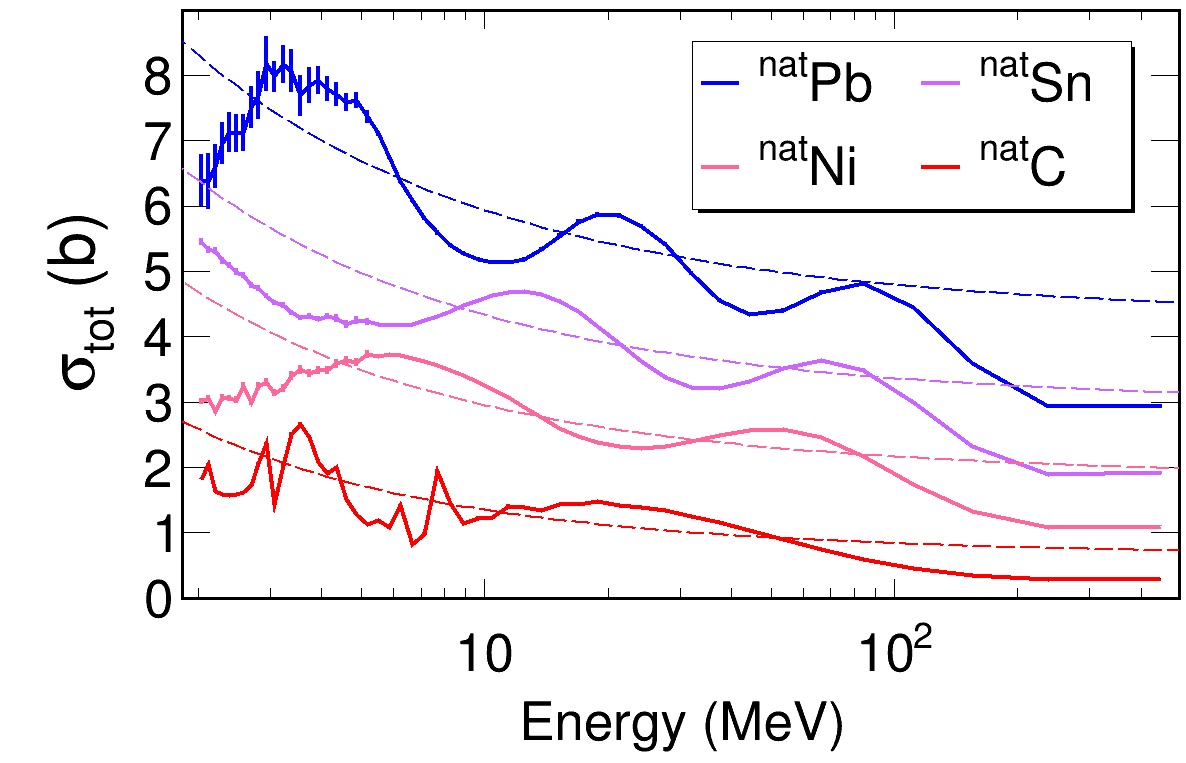
| (1) |
where and is the reduced wavelength of the incident neutron with energy in the center of mass 20; 49. While on average, experimental data comport with this naïve model, the most prominent feature of experimental data is the oscillatory behavior centered about the average of Eq. (1), visible in Fig. 1. Peterson 42 interpreted these oscillations as the result of a phase shift between neutron partial waves passing around the nucleus (thus undergoing no phase shift) and waves passing through the nuclear potential, where they are refracted and exhibit a retardation of phase (an illustration is available in 49).
This explanation was termed the “nuclear Ramsauer effect” by Carpenter and Wilson 13 based on the analogous effect seen in electron scattering on noble gases.
Following Angeli and Csikai 5, this explanation can be incorporated by imbuing the strongly-absorbing-sphere relations with a sinusoidal term:
| (2) |
where and , being the phase difference between a partial wave traveling around and traveling through the nucleus. The large amplitude of the oscillations suggests that elastic scattering accounts for a significant fraction of the total cross section, in turn implying a larger mean free path for neutrons through the nucleus than might otherwise be expected in the absence of Pauli blocking 35; 21. If we approximate the nucleus with a real spherical potential of radius and depth , the total phase shift is:
| (3) |
where is the average chord length through the sphere 5. Rearranging Eq. (3) in terms of and and discarding leading constants yields:
| (4) |
This form reveals an important relation: as is increased, to maintain constant phase , must also increase 49; 42. This is contrary to a typical resonance condition where an integer number of wavelengths are fit inside a potential; in that case, to maintain constant phase as is increased, must be decreased. Thus these oscillations have been referred to as “anti-resonances” or “echoes” 49; 34. Other authors 4 have exposed weaknesses in Angeli and Csikai’s interpretation of Eq. (2) and have provided a more general semi-empirical equation for . However, Eq. (2) is a valuable starting point for connecting with the depth and shape of the nuclear potential as experienced by neutrons.
By including additional surface, spin-orbit, and other terms, OMs have been used to successfully reproduce the general features of all manner of single-nucleon scattering data across the chart of nuclides up to several hundred MeV 39; 55; 28. However, despite the excellent agreement with experiment, OMs involve the interaction of many partial waves with many sometimes-opaque terms in the potential, complicating intuitive understanding of the underlying physics at play. In particular, the isovector components of optical potentials are quite difficult to constrain as they depend on both proton and neutron scattering data, one or both of which are often unavailable. For example, when Dietrich et al. conducted an analysis of neutron total cross section differences between W isotopes, including standard isovector terms in their optical potential worsened the reproduction of experimental relative differences, an illustration of how poorly these isovector components are known 17.
With these considerations in mind, our present goal is twofold: first, to provide new isotopically resolved data useful for identifying the dependence of optical potential terms on nuclear asymmetry; and second, conduct a DOM analysis of these new data along with a large corpus of scattering and bound-state data to extract veiled structural quantities (e.g. neutron skin thicknesses and spectroscopic factors, or SFs) for several cornerstone, closed-proton-shell nuclei. Key findings of this DOM analysis are presented in the companion Letter 45.
II Experimental Considerations
By scattering secondary radioactive beams off of hydrogen targets in inverse kinematics, proton-scattering experiments are possible even on highly unstable nuclides. Because neutrons themselves must be generated as a secondary radioactive beam, neutron-scattering experiments are restricted to normal kinematics and measurements are possible only for relatively stable nuclides that can be formed into a target. At present, measurements above the resonance region on nuclides with short half-lives (shorter than the timescale of days) are technically infeasible for this reason, though a handful have been carried out on samples with half-lives in the tens to thousands of years 44; 43; 24.
Traditionally, measurements have relied on analog-electronics techniques for recording events, techniques that suffer from a large per-event deadtime of up to several . For a typical analog intermediate-energy measurement with dozens or hundreds of energy bins, achieving statistical uncertainty at the level of 1% requires a thick sample to attenuate a sizable fraction of the incident neutron flux. If cross sections are in the 1-10 barn range, this means sample masses of tens of grams 22; 3. Producing an isotopically enriched sample of this size is often prohibitively expensive. As a result, there is a dearth of data on isotopically resolved targets from 1-300 MeV, even for closed-shell isotopes of special importance like 3,4He, 18O, 64Ni, 112,124Sn, and 204,206Pb (see Fig. 1.3 in 46).
Recent developments in waveform digitizer technology have made it possible to reduce the per-event deadtime by an order of magnitude or more, enabling a corresponding reduction in the necessary sample size. In 2008, we embarked on a campaign of measurements on isotopically enriched samples using these new technical capabilities, starting with 40,48Ca from MeV 51. The data from that measurement were incorporated into several DOM analyses 37; 31; 33 that yielded proton and neutron SFs, charge radii, and initial estimates of the neutron skins 32 for these nuclei. Here we significantly expand on that effort by providing results for the important closed-shell nuclides 16,18O, 58,64Ni, and 112,124Sn. We also present a measurement on a very thin sample of the naturally monoisotopic 103Rh to demonstrate that experiments over a broad energy range using only a few grams of material are feasible.
III Experimental Details
All measurements were carried out at the 15R beamline at the Weapons Neutron Research (WNR) facility of the Los Alamos Neutron Science Center (LANSCE) during the 2016 and 2017 run cycles. Our experiment was modeled on previous measurements at WNR 22; 3; 51. At WNR, broad-spectrum neutrons up to 700 MeV are generated by impinging proton pulses onto a water-cooled, 7.5 cm-long tungsten target (Fig. 2). Before the beam enters the experimental area, a permanent magnet deflects all charged particles generated by the proton pulses, allowing only neutrons and rays to reach the experimental area. At the entrance to the experimental area, the beam was collimated to 0.200 inches using steel donuts with a total thickness of 24 inches. In addition, the -ray content of the beam was suppressed using a plug of Hevimet (90% W, 6% Ni, 4% Cu by weight) at the upstream entrance of the collimation stack. After collimation, the beam passed successively through a flux monitor, the sample of interest, a veto detector, and finally the time-of-flight (TOF) detector approximately 25 meters from the neutron source. All detectors consisted of BC-400 fast scintillating plastic mated with photomultiplier tubes (PMTs) and encased in either a plastic or an aluminum housing. The flux monitor and veto detector each had scintillator thicknesses of 0.25 inch and the TOF detector had a scintillator thickness of 1 inch. Signals from all detectors and the target changer were relayed to a 500-MHz CAEN DT-5730 waveform digitizer running custom software. To improve time resolution, the TOF detector used two PMTs (one left, one right) mated to the same plastic scintillator and the PMTs’ signals were summed before digitization.


The particular neutron beam structure at WNR dictates the energy range achievable for measurements (Fig. 3). Proton pulse trains, called “macropulses”, are delivered to the tungsten target at 120 Hz. Each macropulse consists of 350 individual proton pulses, called “micropulses”, spaced 1.8 apart. Each micropulse consists of a single proton packet that generates rays and neutrons within a tight temporal-spatial range. As neutrons from this micropulse travel along the beam path, high-energy neutrons separate in time from lower-energy neutrons so that neutron energy can be determined by standard TOF techniques (see 36 for details). Because the rays and high-energy neutrons from later micropulses can overtake slower neutrons from an earlier micropulse, the distance of the TOF detector from the neutron source determines both the minimum neutron energy that can be unambiguously resolved and the maximum instantaneous neutron flux, critical to correcting for per-event deadtime.
A programmable sample changer with six positions was used to cycle each sample into the beam at a regular interval of 150 seconds per sample. Once per macropulse, an analog signal from the sample changer was recorded to indicate its current position. The flux monitor was used to correct for variations in beam flux between macropulses. The veto detector suppressed events from charged-particle production in the samples and in air along the flight path.
Custom digitizer software was used to run the digitizer in two complementary modes, referred to as “DPP mode” and “waveform mode”. In DPP mode, triggers were initiated by the digitizer’s onboard peak-sensing firmware. For each trigger, several quantities were recorded: the trigger timestamp, two charge integrals over the detected peak with different integration ranges (32 ns for the short integral, 100 ns for the long integral), and a 96-ns portion of the raw digitized waveform, referred to as a “wavelet”. DPP mode was used for the vast majority of the experiment and accounts for 99% of the total data volume. In waveform mode, the digitizer performs no peak-sensing and was externally triggered. Upon triggering, the trigger timestamp and a very long wavelet (60 ) were recorded. While waveform mode data accounts for only 1% of the total data, the instantaneous data rate is much higher than in DPP mode because hundreds of of consecutive waveform samples are stored. Roughly once every three seconds, the digitizer was switched to waveform mode for one macropulse, then switched back to DPP mode as quickly as possible (10-40 ms, depending on run configuration).
Except for the O and Rh samples, all samples were prepared as right cylinders 8.25 mm in diameter and ranging from 10-27 mm in length (see Table 1 for sample characteristics). For each element studied, a natural-abundance sample was also prepared as were two natural C samples and a natural Pb sample, useful for benchmarking against literature data. The samples were inserted into styrofoam sleeves and seated in the cradles of the sample changer. This design minimizes the amount of non-target mass proximate to the neutron beam path. Our samples were generally much smaller than those used in previous measurements; for example, the Ni and Sn samples used in 3; 22 had areal densities of 1.515 and 0.5475 mol/cm2, respectively, 12.7 and 6.5 times larger than for our Ni and Sn samples.
| Isotope | Length | Diam. | Mass | NA | SA | |
|---|---|---|---|---|---|---|
| (mm) | (mm) | (g) | (mol/cm2) | (%) | (%) | |
| C | 13.66(2) | 8.260(5) | 1.2363 | 0.1921(1) | - | - |
| C | 27.29(2) | 8.260(5) | 2.4680 | 0.3835(2) | - | - |
| H2O | 20.00(1) | 8.92(1) | 1.2461 | 0.1107(3) | - | - |
| D2O | 20.00(1) | 8.92(1) | 1.3852 | 0.1107(3) | 0.02 | 99.9 |
| HO | 20.00(1) | 8.92(1) | 1.3844 | 0.1107(3) | 0.20 | 99.9 |
| 58Ni | 7.97(3) | 8.18(2) | 3.6438 | 0.1197(3) | 68.1 | 99.6 |
| Ni | 8.00(3) | 8.20(2 | 3.6898 | 0.1192(3) | - | - |
| 64Ni | 7.96(2) | 8.20(4) | 3.9942 | 0.1192(6) | 0.93 | 92.2 |
| 103Rh | 2.03(1) | 10.20(2) | 2.8359 | 0.02426(4) | 100 | 99.9 |
| 112Sn | 13.65(3) | 8.245(5) | 4.9720 | 0.08332(5) | 0.97 | 99.9 |
| Sn | 13.68(3) | 8.245(5) | 5.3263 | 0.08414(5) | - | - |
| 124Sn | 13.73(3) | 8.245(5) | 5.5492 | 0.08399(5) | 5.79 | 99.9 |
| Pb | 10.07(2) | 8.27(1) | 6.130 | 0.05508(6) | - | - |
The O isotopes were prepared as water samples to increase the areal density of atoms and for ease of handling. Each water sample was contained by a cylindrical brass vessel with thin brass endcaps (0.002 inches), and an empty brass vessel served as the blank. 16,18O cross sections were calculated by subtracting the well-known H cross section from the raw H2O results. We used H data sets from Clement et al. 15 and Abfalterer et al. 3, which together cover the range MeV and are in excellent agreement where their energy ranges overlap. In light of the additional uncertainty inherent to this subtractive determination, we prepared a deuterated water sample, from which the literature for D2 could be subtracted, to serve as an additional cross-check. Due to the poor machining properties of Rh, the 103Rh sample was prepared by purchasing and stacking a series of thin discs rather than by manufacturing a fused cylinder. These discs were held in place by a cylindrical plastic case with open ends.
IV Experimental Analysis
The quantity of interest, , is related to the flux loss through a sample by:
| (5) |
or, equivalently,
| (6) |
where is the neutron flux entering the sample, is the neutron flux transmitted through the sample without interaction, is the number density of nuclei in the sample, and is the sample length. For thin or low-density samples, flux attenuation through the sample will be small (e.g., 13% for our Ni samples at 100 MeV) and a large number of counts will be required to determine the cross section to high precision.
Two post-processing steps were used to improve TOF-detector timing resolution (see Fig. 4). First, the waveform for each TOF-detector event was passed through a software constant-fraction discriminator (CFD) logic, improving precision by a factor of two. Second, a -ray-averaging procedure (cf. 51) was used to improve the precision of each micropulse start time. The final corrected TOF resolution (taken as the FWHM of the -ray peak in the TOF spectra) ranged from 0.60-0.90 ns over the series of measurements. This is comparable to the resolution from our digitizer-mediated measurement on Ca isotopes in 2008 51. For context, for a 100-MeV neutron and a TOF detector distance of 25 meters, a TOF uncertainty of 0.80 ns translates to an energy resolution of 900 keV. For neutrons below 20 MeV, the TOF time resolution worsens because the traversal time through the 1-inch thickness of the TOF detector becomes non-negligible. However, because the TOF of these neutrons is already very long (several hundred ns or longer) the relative energy resolution () is superior at low energies. As an example from one of our runs, a 5 MeV neutron with a 0.82 ns detector-traversal time and an inherent TOF resolution of 0.80 ns has an energy uncertainty of 13 keV. These energy uncertainties have been propagated through subsequent analysis into our results below.
Calculating the neutron energy requires knowledge of the flight-path distance to high precision. We determined this distance by calculating putative data for C from 3-15 MeV from our measurement and comparing the resonance peaks in this region with high-precision literature data sets. From this study, the mean TOF distance was determined as 2709 1 for the Ni and Rh run configuration and 2554 1 for the Sn and O run configuration.

Before cross sections could be tabulated, the per-event deadtime had to be modeled and corrected for. Because events are not processed instantaneously, there is a brief period after each trigger during which the digitizer is busy processing that trigger. Any newly arriving events in this period will be ignored, privileging events arriving earlier and thus distorting TOF spectra and resulting cross sections. This busy period is referred to as the “analytic” or “per-event” deadtime and can be corrected for according to standard techniques 36. An additional complication is the possibility of flux variation between micropulses. If there is no variation, the fraction of time that the digitizer is dead for a given time bin can be calculated 36:
| (7) |
where is the number of time bins in the micropulse, is the rate of detected events per micropulse in bin , and is the probability that the digitizer is still busy from a trigger bins ago. If the variation in beam flux is significant, a more advanced formula can be used; however, an examination of our flux-per-micropulse data showed very little flux variance across macropulses, except during the first 10% of the micropulses within each macropulse. In the final analysis we discarded these first 10% and used the simpler Eq. (7) to calculate the dead time fraction.
To model the experimentally observed probability-dead, , we fitted a logistic function to the observed spectrum for time differences between consecutive events (Fig. 5). For a given bin , the fraction of time that the digitizer is dead, , is a discrete convolution of the measured TOF spectrum with . Note that except for the first and last micropulses in a macropulse, all micropulses are consecutive, so deadtime effects can “wrap around” from the end of one micropulse to the next. For these wrap-around contributions (that is, ), the (mod ) term ensures that the bin referred to by is non-negative.
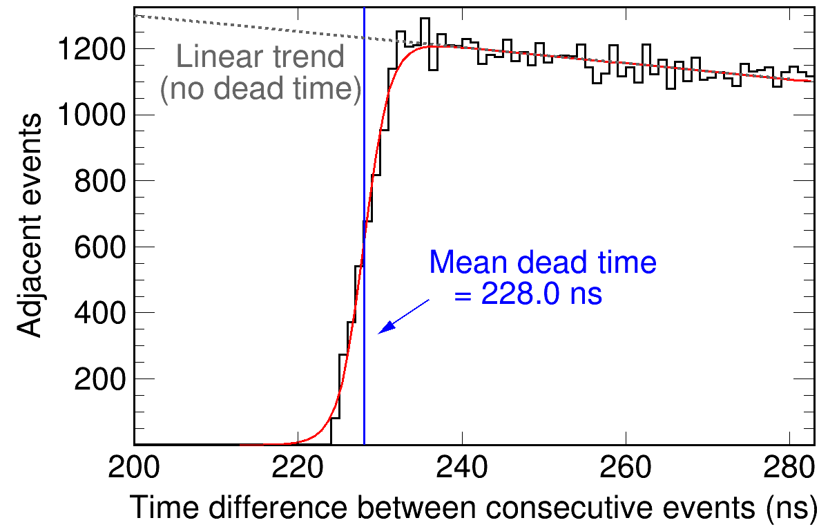
Because trigger processing is done in firmware onboard the digitizer, the per-event deadtimes affecting our measurement were reduced to between 150-230 . After we calculated the average probability-dead for each time bin, the total number of events detected in that bin, , could be corrected to recover the true number of events that would have been detected in the absence of a per-event deadtime:
| (8) |
where is the total number of micropulse periods. At large TOFs (low energies) the correction is as low as a few percent, but at small TOFs (high energies), the digitizer is often still dead from the -ray flash and high-energy neutrons. In this regime the correction can be quite large (20% for our Ni/Rh runs, and 40% for our Sn/O runs). Still, the corrections needed for our measurement are far smaller than the typical analytic deadtime corrections required with the deadtime mitigation scheme of previous analog measurements 22; 3.
In addition to analytic deadtime, there is an additional deadtime effect associated with digitizer readout to the data acquisition computer (DAQ). During data collection, each pair of digitizer channels shares a common buffer for storing events. After several seconds of acquisition, the digitizer begins readout at which time the acquisition is paused and buffer contents are read out to the DAQ. However, because each buffer is independently read out to the DAQ, it is possible that buffers could be emptied and readied for new acquisition at slightly different times (10-40 ms apart), and a mismatch could develop between the number of macropulses seen on different channels. Such run-time interactions between the firmware and USB traffic of the DAQ were difficult to characterize, but we estimate that they might cause a systematic error of a few tenths of one percent in the number of macropulses seen by different channels, depending on the user-defined threshold and the buffer size. This effect could contribute to the discrepancy at the highest energies (100 MeV) between our results and past analog-enabled measurements.
During analysis, it was noted that occasionally (1 in 400 macropulses), one or two adjacent macropulses would have an abnormally small number of events. The frequency of these “data dropouts” was similar to the rate of switching between DPP and waveform modes; we suspect it is related to edge case behavior right before or after a mode switch. To mitigate this issue, we threw out any macropulse that had less than 50% of the average event rate in either the flux monitor or TOF detector channel.
After applying these corrections, the veto and integrated charge gates were applied to all events and surviving events were populated into TOF spectra (Fig. 6). Next, room background was subtracted (responsible for 0.1% to 1% of event rate, depending on energy) and spectra were mapped to the energy domain.
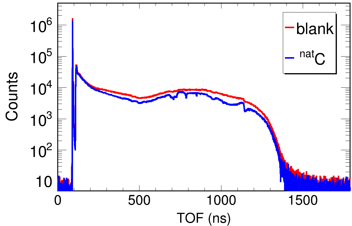
From these energy spectra, the raw cross sections were calculated, bin-wise, as follows:
| (9) |
where / is the ratio of counts in the energy spectra between the blank and sample, / is the ratio of counts in the monitor detector between the sample and blank (for flux normalization).
Finally, two isotope-dependent corrections were applied to the raw cross sections. First, because the blank sample contains air and not vacuum, the cross section of air must be added to each sample’s cross section. Second, the cross section for 64Ni was corrected for the isotopic enrichment of our sample (92.2%) using our measured Ni cross section. All other isotopes were sufficiently pure such that the impurity correction was negligible.
To validate our analysis, we first benchmarked our measurements of natural samples (C, Ni, Sn, and Pb) against the high-precision data sets on natural samples from 22 and 3 (Fig. 7). Our natural sample results are in excellent agreement with these previous results from 3-100 MeV and show slight deviation above 100 MeV (a relative difference of up to 5% at 300 MeV), suggesting a small systematic error at high energies in one or both approaches when the instantaneous neutron flux is highest. As an additional diagnostic, we compared results from our long and short natural carbon targets and found excellent agreement, within 1% throughout the measured energy domain.
Extracting the 16,18O required subtraction of the well-measured for H. To better characterize the additional systematic uncertainty associated with this subtractive analysis, we subtracted our measured values for 16O neutron from our raw D2O and H2O data and calculated the D-to-H relative difference. A comparison of our D-to-H relative difference with that of 1 is shown in Fig. 8. Our results differ systematically from the previous (analog) measurement by 2-3% throughout the energy range, comparable to the 2% systematic difference between our final 16O neutron results and those of 3. The size and uniformity of these systematic differences is consistent with a combination of slight (1%) normalization errors in some or all of the H, D, O, and C neutron results from our measurement or in the literature data.


V Experimental Results
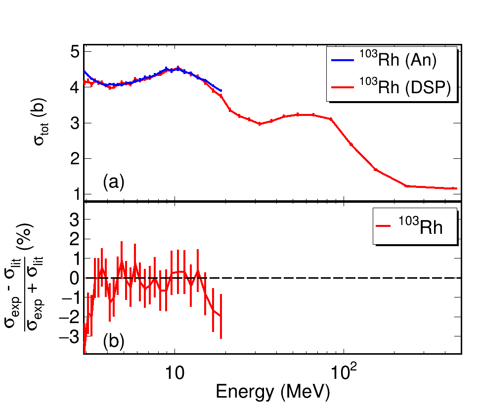
Our absolute results for O, Ni, and Sn isotopic targets are shown in Fig. 9. Results for Rh are shown in Fig. 11. Literature isotopic measurements (where they exist) are shown alongside our results for comparison. Residuals between our data and any existing literature data are also shown. In each figure, the literature data sets have been rebinned to match the bin structure of our data to facilitate comparison. In regions with a low density of states where individual resonances are visible (e.g., C below 10 MeV), this rebinning washes out the fine structure of the cross sections.
Except for the already well-measured 16O, our new data significantly extend knowledge of the neutron for each sample. In the cases of 18O, 58Ni, 103Rh, and 124Sn, almost no previous data were available above 20 MeV. Our new data are in good agreement with the previous measurements where available. In the cases of the rare isotopes 64Ni and 112Sn, data were available at only one energy, 14.1 MeV, from a study from more than 50 years ago 18 and our measurement is in excellent agreement, within 2-3%.
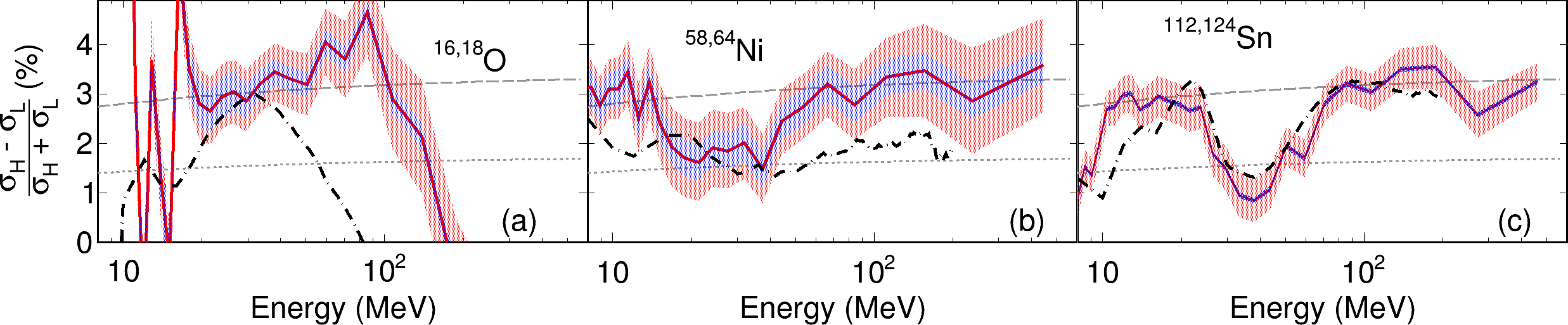
Our results for relative differences between isotopic pairs 16,18O, 58,64Ni, and 112,124Sn are shown in Fig. 10. For 16,18O [Fig. 10(a)], the purely isoscalar SAS model [Eq. (1)] grossly reproduces the relative difference below 100 MeV, but fails completely above 100 MeV. Near 200 MeV, the 18O crosses over that of 16O resulting in a negative relative difference, in keeping with the Ramsauer-logic expectation of Eq. (2) that oscillation minima shift to higher energies as is increased. In the relative difference subfigures for 58,64Ni and 112,124Sn [Fig. 10(b) and 10(c)], the average values are below the SAS model trend (), shown by the dashed lines. The well-known trend in Sn isotope-shift data 7 is also shown for reference and underpredicts the relative differences. In the DOM analyses presented below, we fit only absolute data and did not directly fit these relative differences. Still, the relative differences between our individual DOM fits for 58,64Ni and 112,124Sn (black dashed-dotted lines) show overall agreement with the experimental relative differences, especially for the Sn relative difference. For the 16,18O relative difference, there is an obvious phase mismatch between the oscillations of DOM calculation and the experimental data. This mismatch is symptomatic of a slight DOM overestimation of the 16O radius (0.02 fm), which nudges the DOM-calculated 16O rightward so that the 18O crossover occurs at too low an energy. As was noted by Dietrich et al. in their study of relative differences in W isotopes, a simultaneous OM analysis along the entire isotopic chain, as in 37, may be required to realize the full isovector-constraining power latent in the relative differences.

VI DOM Analysis
The DOM is a phenomenological Green’s-function framework enabling a simultaneous and self-consistent analysis of nuclear structure and reaction data. An essential feature of the DOM is the enforcement of a dispersion relation between the complex components of the self-energy across the entire energy domain, allowing structural data from below the Fermi energy (e.g., charge densities, bound levels) to help constrain the potential above, and data from above the Fermi energy (e.g., elastic, reaction, and total cross sections) to help constrain the potential below. Using our new data for 16,18O, 58,64Ni, and 112,124Sn, we performed a simultaneous fit on each isotopic pair and also revisited 40,48Ca and 208Pb. Compared to previous DOM analyses 37; 9; 31; 32, we employ an updated version of the DOM that has been generalized for use with any combination of near-spherical even-even nuclei. Partial occupation of neutron open shells, as for the neutron d5/2 valence shell in 18O, is accommodated using the level’s energy and the pairing parameter :
| (10) |
where is the binding energy of the nucleus with neutrons and protons. Occupation for the level is split into upper () and lower () components:
| (11) |
where , . Only the lower (occupied) component is included in calculations of bound-state quantities (e.g., total particle number, binding energy).
In the appendices, we provide the functional forms used to define the potential (Appendix A), optimized parameter values with uncertainties (Appendix B), and figures showing the quality of the DOM reproduction to each experimental data set (Appendix C). The other major methodological difference is the use of Markov-Chain Monte Carlo (MCMC) for parameter optimization, discussed below.
For additional details on the underlying DOM formalism, see 30; 16. To calculate cross sections from the self-energy, the standard R-matrix approach was used 29. Except where indicated, experimental data used for fitting are the same as in 46. To situate the reader, we describe the corpus of experimental data and DOM results for 16,18O in full detail. The experimental data used and fit quality for 40,48Ca, 58,64Ni, 112,124Sn, and 208Pb are similar in quantity and quality and only key differences are noted. For systematics of neutron skins and binding energies, see companion Letter 45.
VI.1 16O experimental data used in DOM analysis
For protons, twenty-eight differential elastic cross sections data sets and twenty analyzing power data sets from 10-200 MeV were incorporated. Only three proton reaction cross section data sets, ranging from 20-65 MeV, were available. As an added constraint, we used systematic trends from the comprehensive proton review of Carlson 12 to generate proton pseudo-data from 70-200 MeV, which were included in the fit. These pseudo-data are shown as gray open symbols in the proton figures in Appendix C. For neutrons, ten differential elastic cross section data sets from 10 MeV to 95 MeV, a single neutron reaction cross section data point at 14 MeV, and our newly measured results for 16O were included. In all, over sixty experimental nucleon scattering data sets were used to constrain the 16O parameters.
In addition to nucleon scattering data, several sectors of bound-state data were included in the fit. Neutron (proton) 0p1/2 and 0d5/2 single-particle level energies were assigned according to the nucleon separation energies of 16O and 17O isotopes (16O, 17F isotopes) 59. Charge density distributions were taken from the compilation of 58. Since the time of that compilation, new experiments (particularly muonic-atom measurements) have improved the precision of many root-mean-square (rms) charge radii by roughly an order of magnitude 6. To account for these improved data, we rescaled the distributions from 58 to recover the updated rms charge radii while still conserving particle number. We also fitted directly to the updated rms charge radii of 6. Because the DOM self-energy does not necessarily conserve particle number, we included the “experimental” proton and neutron numbers of eight as part of the fit. Lastly, the total binding energy of 16O from 59 was included as a constraint.
VI.2 18O experimental data used in DOM analysis
Extensive proton elastic scattering data for 18O was available from the EXFOR database. Twenty-eight proton elastic differential cross sections were included ranging from 10-200 MeV. Unfortunately, no proton reaction cross section data were available at all in the relevant range of 10-200 MeV. As with 16O, we generated proton reaction cross section pseudo-data from systematic trends in 12 from 70-200 MeV. On the neutron side, two differential elastic cross section data sets were included, at 14 and 24 MeV, but no analyzing powers were available. One datum for the neutron reaction cross section, at 14.1 MeV, was incorporated as well. Our results for 18O were the sole neutron total cross section data used in the fit. The energies of the proton and neutron 0p1/2 and 0d5/2 single-particle levels were assigned according to the same procedure used for 16O.
Unlike 16O, for 18O, no charge density distribution was available from 58. To approximate it, we rescaled the charge density distribution used for 16O to give the 18O rms charge radius of 6 while preserving eight units of charge. As with 16O, we also fitted to the experimental rms charge radius directly, to the particle numbers and , and the total binding energy.
VI.3 MCMC analysis
Several aspects of the DOM potential make optimization challenging. Even with the reduced number of potential parameters used in this work (42 for 208Pb and 43 for all other pairwise fits) compared to past DOM studies (for example, 60 or more in 32), we found that classical gradient-descent methods were inappropriate for reliably searching the parameter space. A recent study 27 systematically compared Bayesian optical model optimization techniques to frequentist ones, the type almost universally used in previous analyses, and found that traditional algorithms may be overconfident in their parameter estimation. To avoid these problems, we used the affine-invariant MCMC library, emcee 23, for optimization and uncertainty characterization. For an in-depth introduction to applied MCMC, see 52.
In the ensemble-sampling approach, several hundred “walkers” are first randomly initialized in parameter space for each isotopic system to be fitted. At each subsequent step during the random walk, each walker’s position is updated from either by accepting a new position with probability:
| (12) |
or by remaining in the same position with probability . New positions are proposed according to the stretch-move proposal distribution of 25 (for our stretch move scaling, we used instead of the default , which improved the typical acceptance fraction from around 5% to 15%). In Eq. (12), the utility of a parameter vector conditional on the experimental data was defined according to Bayes rule (omitting the evidence term):
| (13) |
where is the full set of constraining experimental data. The parameter prior distribution was specified as uniform over a physically reasonable range for each parameter. For example, the diffusenesses of all Woods-Saxon potential geometry terms were restricted to 0.4-1.0 fm. Other more sophisticated choices for the prior distribution (e.g., broad truncated Gaussians) were tested and had little impact on the resulting posterior distributions. The likelihood function was defined as a least-squares function over all data sectors :
| (14) |
where
- •
is the number of experimental data points in a data sector ,
- •
are the calculated and experimental values, respectively, for the datum of sector ,
- •
are the assigned model and experimental errors, respectively, for the datum of sector .
Appendix A shows the parameter definitions and prior distributions used in the present analysis.
Due to the choice of functional form and finite model basis size, DOM predictions for nuclear observables suffer from inherent model error. For example, many previous OM analyses tend to easily reproduce low-angle experimental data taken at lower scattering energies but are increasingly discrepant with the data at high energies and at backward angles, where the predicted cross sections may differ from experimental results by an order of magnitude or more. This discrepancy indicates a deficiency in the potential form of the OM; ignoring it can lead to drastic underestimation of variances of extracted quantities. In this investigation, we found that the inclusion of reasonable model discrepancy terms in our utility function improved the visual fit to experimental data while broadening parameter uncertainties, in keeping with the methodological findings of 11. Table 2 shows the model error terms we used for each data sector. We assigned model error for each data set according to how well preliminary fits could reproduce differing regions of each data sector, the flexibility of the functional forms, and intuition from the successes and failures of past OM analyses. In principle, the form of these model error terms could also be treated as random variables to be sampled over during MCMC, but due to computational limitations and the already-challenging size of the DOM parameter space, we elected to fix the model error terms. After samples have been taken from the posterior distribution, a subset can be used to estimate the true parameter distributions, and physics results calculated for each sample. Ensuring that this subset is representative of the true posterior is discussed in the next section.
| (%/) | (-) | (%) | (%) | (MeV) | (%) | (-) | (fm) | (%) |
| 0.25 | 0.10 | 0.25 | 0.25 | 0.10 | 5.0 | 0.10 | 0.005 | 1.0 |
Following 23 we attempted an autocorrelation analysis to test for convergence and estimate the number of independent samples we had collected for each nucleus. Because of computational limitations on the number of walkers and steps used to approximate the posteriors, posterior estimation involves a finite MCMC sampling error. The integrated autocorrelation time for a physics feature , denoted , represents the number of steps required for a walker to produce a new, decorrelated posterior sample for the feature that is independent of the previous independent sample. In an ideal MCMC analysis, could be accurately computed for each physics quantity and the MCMC sampling error could be robustly estimated. In practice, we found this to be computationally infeasible for the DOM parameter space. For example, in preliminary analysis of 18O, we were able to perform steps for each of 336 walkers (more than 100,000 CPU-hours in total). Over this domain, we calculated the integrated autocorrelation time for each potential parameter , denoted , to be roughly 2800 steps. Assuming a rule-of-thumb condition for convergence of the estimate near its true value, the decorrelation time appears to be extremely long. In other words, from alone, we could not exclude the possibility that the parameters had not yet fully “settled” in the region of their optimal values and begun independent sampling of the parameter posteriors. We note that the true could be considerably smaller than due to the highly correlated nature of DOM parameter space.
To proceed, we applied several commonsense tests to judge whether our parameter and extracted-quantity estimates were accurate. First, we sampled as long as possible and used as many parallel walkers as possible, given our computational resources. From time to time during sampling, we analyzed the mean walker positions and the mean walker position likelihood as a function of sampling step. Encouragingly, for all nuclei walkers quickly converged on a common region (within 1000 samples) and their mean parameter values stabilized soon afterward (within 10000 samples), suggesting that walkers were sampling a reasonably optimal subspace. At this point, we considered the chain tentatively converged. As an additional test, we re-started sampling from a different (uniformly random) initial position for each nucleus and found that a similar optimal subspace was reached, again within roughly 1000 samples, indicating that our results are independent of the initial walker positions. Finally, for a “converged” chain, we calculated extracted physics quantities (e.g., neutron skins, scattering cross sections) for all walkers at several intervals to confirm that their mean values were stable. Again using 16O and 18O as an example, we found their mean neutron skin values varied by less than 0.001 and 0.01 fm, respectively, over several thousand sampling steps late in sampling. Out of caution (and given our expectation of very large autocorrelation times) we used only the terminal sample for each walker chain to produce the results presented here and in the companion Letter 45. In the end, we expect that additional sampling could slightly reduce the estimated variance of each extracted quantity but have a negligible effect on the mean values. For all quantities derived from MCMC analysis, the estimated 16th, 50th, and 84th posterior percentile values are denoted as . The range between the 16th and 84th percentiles corresponds to a 1-uncertainty range if the posteriors are assumed to be Gaussian. The median values and ranges for each parameter for each isotope system are listed in Appendix B.
VI.4 Fit results on 16,18O
Figure 12 in Appendix C shows the DOM fit of 16O and experimental data. The experimental proton , neutron , , and charge density distribution, binding energy per nucleon, and p1/2 and d5/2 single-particle energy data are all well-reproduced suggesting that the DOM is effective for modeling nuclei as light as =16. Almost all experimental proton data are accurately reproduced by the DOM calculations with the exception of an overprediction of cross sections at backward angles and high energies, a regime known to be challenging from past OM analyses. In addition, the median DOM-generated rms charge radius, 2.72 fm, slightly exceeds the experimental value of 2.70 fm. Taken together with the 16,18O relative difference results in panel (a) of Fig. 10, these overestimations indicate that the traditional OM assumption of radial proportionality with must be tweaked for a better description of 16O.
To reproduce the 16O proton pseudo-data generated from 12, a larger volume imaginary term was required above 100 MeV, which in turn reduced the spectroscopic strength for the valence and p1/2 nucleons by roughly 0.05. We also note the importance of the charge density distribution for determining the magnitude of the imaginary strength below the Fermi energy. For example, in test fits where the charge density was not included as a constraint, most of the negative imaginary strength was concentrated in the surface term between MeV, and the tail of the charge density was overpredicted. With the charge density included as a constraint, the imaginary surface magnitude shrank by a factor of two and the volume term grew to compensate, pushing nucleon density deeper in energy space and increasing the binding energy closer to the experimental value.
While all data sectors contributed at least some information not fully captured by any other sector, the proton , neutron , and charge density provided the most stringent constraints on the self-energy. The analyzing powers were the most difficult sector of experimental data to reproduce, with moderate deviations visible from 10-15 MeV for both protons and neutrons and above 100 MeV for protons [Figs. 12(b) and 12(d)]. Some of the difficulty with the analyzing powers is attributable to our neglecting of an imaginary spin-orbit term in the DOM potential used in this work, a choice made due to the unreasonable unbounded growth of the imaginary spin-orbit term as grows in the traditional definition used in 28. In a future analysis we intend to quantitatively investigate the importance of the imaginary spin-orbit term and to compare different options for its functional form.
Figure 13 in Appendix C shows the 18O experimental data and the DOM fit. The paucity of 18O experimental data presented a challenge for our analysis. To constrain the negative-energy domain of the potential, the only unambiguous experimental data were the neutron and proton separation energies and the overall binding energy. As with 16O, broad agreement with experimental data was achieved for experimental proton and neutron data, the neutron , rms charge radius, binding energy per nucleon, and p1/2 and d5/2 single-particle energy data. The artificially scaled charge density and proton data were also easily reproduced. Due to the deterioration of systematic trends from 12 below 70 MeV, we did not generate proton pseudo-data for lower energies, so the positive-energy surface term of the potential was largely unconstrained in this important area.
| Isotope | 16O | 18O | 40Ca | 48Ca | 58Ni | 64Ni | 112Sn | 124Sn | 208Pb | ||
|---|---|---|---|---|---|---|---|---|---|---|---|
| Level | 0p1/2 | 0p1/2 | 0d3/2 | 0d3/2 | 0f7/2 | 0f7/2 | 0g9/2 | 0g9/2 | 2s1/2 | ||
| SF | |||||||||||
| Level | 0p1/2 | 0d5/2 | 0d3/2 | 0f7/2 | 1p3/2 | 1p3/2 | 1d5/2 | 0h11/2 | 1f5/2 | ||
| SF | |||||||||||
In symmetric 16O, the proton and neutron potentials were identical except for the Coulomb interaction, so the neutron data provided information about both the proton and neutron imaginary strength at positive energies. For 18O, this expectation of symmetric potentials was inapplicable, making proton data essential for fixing the positive-energy imaginary strength for protons. In principle, 18O proton and neutron differential elastic scattering cross sections about 100 MeV could jointly yield some information about the asymmetry-dependence of the imaginary strength for 18O, but no neutron elastic scattering data were available above 24 MeV. For a better characterization of this nucleus, even a single proton datum between 10 and 50 MeV would be valuable.
VI.5 Fit results for
40,48Ca, 58,64Ni, 112,124Sn, and 208Pb
Figures 14-20 in Appendix C show 40,48Ca, 64Ni, 112,124Sn, and 208Pb experimental data and the DOM fits. The availability of single-nucleon scattering data for 40,48Ca, 58,64Ni, 112,124Sn, and 208Pb followed the same trends as that for 16,18O: plentiful proton differential elastic scattering data, moderate coverage for neutron differential elastic cross sections and proton reaction cross sections on abundant isotopes (40Ca, 58Ni, and 208Pb), with little-to-no coverage for neutron scattering or proton reaction cross section data on rare isotopes (48Ca, 64Ni, 112Sn, 124Sn). For 112Sn and 124Sn, however, even proton elastic scattering data sets were sparse and no data above 50 MeV were available, making our newly collected neutron data especially valuable in constraining the potential. For 40Ca and 208Pb, experimental proton reaction cross section data were available up to 200 MeV; for the other isotopes, proton reaction cross section pseudo-data (discussed in the 16,18O subsections) were used as a constraint. As for 18O, no charge-density parameterization was available for 112Sn in 58, so we rescaled the available 124Sn distribution to reproduce the 112Sn charge radius.
Generally, all sectors of experimental data were well-reproduced; exceptions include the high-angle (above 120) proton elastic scattering data for 40Ca and 208Pb, where data sets were available up to 200 MeV, and the single-particle energies for neutron open shells in 112,124Sn (see Figs. 18 and 19), where several levels are partially filled and clustered near the Fermi surface. Achieving more accurate single-particle energies while preserving particle number accuracy may require a more sophisticated treatment of pairing. Our new neutron data were well-reproduced across the board, typically within 2% of the experimental value, by the DOM fits, suggesting that our Lane-like parameterization of the potential’s asymmetry dependence [Eqs. (29-32)] is a promising starting point for extrapolation away from stability. We note that because 208Pb was fit on its own without an isotopic partner, initial fits showed that the asymmetry-dependence of the HF radius term was too poorly constrained to yield reliable neutron skin results; in the final treatment, this term was disabled for 208Pb.
VI.6 Discussion
Table 3 shows DOM-calculated SFs for valence proton and neutron levels for all nine systems. Significant depletion from the mean-field expectation appears even in the light systems 16,18O. In the present study, the extracted proton SFs show only a very weak dependence on neutron-richness within each isotopic pair, in keeping with the weak dependence extracted in and transfer reaction studies and at odds with knockout-reaction analyses that recover a strong asymmetry-dependence 54; 16. The recent DOM analyses of 9; 8 identified proton reaction cross sections above roughly 100 MeV as important for their successful reproduction of 40,48Ca cross sections without arbitrary SF rescaling. Compared to the present work, these analyses found a much larger reduction of valence proton SFs in 48Ca with respect to 40Ca, indicative of an SF asymmetry dependence somewhere between the weak dependence deduced from transfer reactions and the very strong dependence from knockout reactions.
To understand the differences between these analyses, we conducted several diagnostic runs with artificially scaled Carlson pseudo-data in 48Ca. These diagnostic runs confirmed that fitting to appropriate high-energy proton reaction cross sections leads to larger 48Ca proton imaginary strength both far above and far below the Fermi energy, an effect already seen in previous DOM work. However, the growth we observed in the imaginary potential was more modest compared to previous treatments, potentially explaining the weaker asymmetry-dependent SF reduction. We also note that in the present work, the high-energy neutron total cross sections and proton reaction cross sections appeared to have little impact on other extracted quantities such as neutron skins, as had been previously hypothesized for the neutron skin of 48Ca 32. We conclude that the different methodological choices, especially the focus of this work on simultaneous fitting of isotope pairs, is responsible for the differences in these asymmetry-dependent quantities. To further clarify the situation, the potentials of the present work should be used to generate cross sections that can be compared to the previous findings of 8.
Surprisingly, despite the extensive proton and neutron elastic scattering data for 16O, 40Ca, and 208Pb, the extracted spectroscopic factor distributions and parameter uncertainties for these isotopes are just as wide as for those systems with barely any available elastic scattering data, such as 64Ni. We tentatively conclude that the elastic scattering data we used are very weak constraints on the all-important imaginary terms of the optical potential, at least for the stable, spherical systems discussed here. Unfortunately, this suggests that elastic scattering measurements in inverse kinematics on radioactive beams are of diminishing utility for extrapolating optical potentials away from -stability. A program of proton reaction cross section and neutron total cross section measurements on radioactive targets could be useful for understanding the potential’s near-Fermi-level asymmetry dependence but is experimentally daunting. Instead, a two-pronged approach may be required. On the experimental side, proton reaction and neutron total cross section measurements on stable isotopic chains can help identify which asymmetry-dependence forms are justifiable for increasingly asymmetric systems. On the theoretical side, sensitivity studies are needed to clarify how bound-state data on highly asymmetric systems connect to scattering cross sections.
Lastly, a few systematics in optical potential parameter values are worth mention. For most of the parameters, there was minimal variation with nuclear size or asymmetry, suggesting that a global DOM treatment using the functional forms we have selected is achievable. The radial term for the real central potential () and for the positive-energy imaginary volume and surface () are nearly constant among 40,48Ca, 58,64Ni, 112,124Sn, and 208Pb, but the values for 16,18O show moderate deviations, another indication that the geometric form of the potential is insufficient for light systems. As a consequence of the limited negative-energy data available for fitting, the negative energy geometric terms () show large variation. The nonlocalities for the negative imaginary components are systematically larger than those for the positive imaginary components. This suggests that while traditional OMs have been able to successfully reproduce positive-energy scattering data with strictly local potentials, description of hole properties requires true nonlocal character in the negative-energy potential. In practice, we found it impossible to simultaneously reproduce charge density distributions, binding energies, and scattering data unless the central potential and at least the volume imaginary terms were equipped with a nonlocality. In the end, for simplicity and generality, each element of the potential (except Coulomb) was treated nonlocally, but it is unclear which particular data are most important for constraining these several nonlocalities. As one moves further from stability to systems with even less (or no) scattering data available, the risk of overfitting will loom until this issue is resolved.
In preliminary fits, the imaginary volume magnitude () component of the potential was shown to be strongly sensitive to the inclusion of the binding energy as a constraint during fitting. We expect the asymmetry-dependence of this term, (), to impact DOM-based predictions of the Ca, Ni, and Sn neutron driplines (as in 37), though in this work, this dependence was very poorly constrained due to the absence of experimental asymmetry-dependent data probing the most deeply bound nucleons. Because they encode information about how protons and neutrons share energy throughout the nucleus, experimental neutron-skin thicknesses could provide this kind of valuable information. For the Ca, Ni, Sn, and Pb fits, the median positive-energy surface imaginary magnitude () is positive, indicating enhancement in proton surface imaginary strength with increasing neutron richness, and a corresponding decrease for neutron surface imaginary strength. Of course, the nuclei under study in the present work are stable; the trend for nuclei with large asymmetries, relevant for the r-process neutron-capture rate, is unknown.
VII Conclusion
By adopting a digitizer-driven approach, we measured on the important closed-shell nuclides 16,18O, 58,64Ni, and 112,124Sn across more than two orders of magnitude in energy (3-450 MeV). Except at the highest energies, our results on natural targets are in good agreement with previous analog-mediated measurements that required 10-20 times more target material.
Using these new data and a suite of scattering and bound-state literature data on 16,18O, 58,64Ni, and 112,124Sn, we extracted DOM potentials capable of reproducing a diverse range of scattering and structural data for both neutrons and protons, validating the use of the DOM away from doubly closed shells from =16 to =208, though with indications that the traditional radial dependence may require modification for light systems. These analyses further indicate that simultaneous fits of isotopically resolved neutron , proton , and charge-density distribution data on isotopic partners provide a more stringent constraint on the asymmetry-dependence of both real and imaginary components.
VIII Acknowledgements
This work is supported by the U.S. Department of Energy, Office of Science, Office of Nuclear Physics under award numbers DE-FG02-87ER-40316, by the U.S. National Science Foundation under grants PHY-1613362 and PHY-1912643, and by the National Nuclear Security Administration of the U.S. Department of Energy at Los Alamos National Laboratory under Contract No. 89233218CNA000001. C.D.P. acknowledges support from the U.S. Department of Energy SCGSR Program (2014 and 2016 solicitations) and the National Nuclear Security Administration through the Center for Excellence in Nuclear Training and University Based Research (CENTAUR) under grant number DE-NA0003841. Computations were performed in part using the facilities of the Washington University Center for High Performance Computing, which were partially provided through NIH grant S10 OD018091, and in part under the auspices of the U.S. Department of Energy by Lawrence Livermore National Laboratory under Contract DE-AC52-07NA27344.
References
- Mahzoon et al. (2017) M. H. Mahzoon, M. C. Atkinson, R. J. Charity, and W. H. Dickhoff, Phys. Rev. Lett. 119, 222503 (2017), URL https://link.aps.org/doi/10.1103/PhysRevLett.119.222503.
- Fattoyev and Piekarewicz (2012) F. J. Fattoyev and J. Piekarewicz, Phys. Rev. C 86, 015802 (2012), URL https://link.aps.org/doi/10.1103/PhysRevC.86.015802.
- Viñas et al. (2014) X. Viñas, M. Centelles, X. Roca-Maza, and M. Warda, Eur. J. Phys. A 50, 27 (2014), URL https://doi.org/10.1140/epja/i2014-14027-8.
- Brown (2000) B. A. Brown, Phys. Rev. Lett. 85, 5296 (2000), URL https://link.aps.org/doi/10.1103/PhysRevLett.85.5296.
- Fernbach et al. (1949) S. Fernbach, R. Serber, and T. B. Taylor, Phys. Rev. 75, 1352 (1949), URL https://link.aps.org/doi/10.1103/PhysRev.75.1352.
- Satchler (1980) G. R. Satchler, Introduction to Nuclear Reactions (John Wiley And Sons, 1980).
- Peterson (1962) J. M. Peterson, Phys. Rev. 125, 955 (1962), URL https://link.aps.org/doi/10.1103/PhysRev.125.955.
- Finlay et al. (1993) R. W. Finlay, W. P. Abfalterer, G. Fink, E. Montei, T. Adami, P. W. Lisowski, G. L. Morgan, and R. C. Haight, Phys. Rev. C 47, 237 (1993), URL http://dx.doi.org/10.1103/PhysRevC.47.237.
- Schwartz et al. (1974) R. B. Schwartz, R. A. Schrack, and H. T. Heaton II, Tech. Rep. 138, National Bureau of Standards (1974).
- Poenitz and Whalen (1983) W. P. Poenitz and J. F. Whalen, Tech. Rep. 80, Argonne National Laboratory (1983).
- Abfalterer et al. (2000) W. P. Abfalterer, R. W. Finlay, and S. M. Grimes, Phys. Rev. C 62, 064312 (2000), URL https://link.aps.org/doi/10.1103/PhysRevC.62.064312.
- Abfalterer et al. (2001) W. P. Abfalterer, F. B. Bateman, F. S. Dietrich, R. W. Finlay, R. C. Haight, and G. L. Morgan, Phys. Rev. C 63, 044608 (2001), URL http://dx.doi.org/10.1103/PhysRevC.63.044608.
- Carpenter and Wilson (1959) S. G. Carpenter and R. Wilson, Phys. Rev. 114, 510 (1959), URL http://journals.aps.org/pr/pdf/10.1103/PhysRev.114.510.
- Angeli and Csikai (1970) I. Angeli and J. Csikai, Nucl. Phys. A 158, 389 (1970), URL http://www.sciencedirect.com/science/article/pii/0375947470901909.
- Mohr (1955) C. B. O. Mohr, Proc. Phys. Soc. A 68, 340 (1955), URL http://stacks.iop.org/0370-1298/68/i=4/a=410.
- Feshbach (1958) H. Feshbach, Ann. Rev. Nucl. Part. Sci. 8, 49 (1958), URL https://doi.org/10.1146/annurev.ns.08.120158.000405.
- McVoy (1967) K. W. McVoy, Ann. Sci. 43, 91 (1967), URL http://www.sciencedirect.com/science/article/pii/000349166790293X.
- Ahmad et al. (1973) I. Ahmad, N. Bano, and A. N. Saharia, Pramana - J. Phys. 1, 188 (1973), URL https://link.springer.com/article/10.1007/BF02847190.
- Perey and Perey (1976) C. M. Perey and F. G. Perey, Atom. Data Nucl. Data Tables 17 (1976).
- Varner et al. (1991) R. L. Varner, W. J. Thompson, T. L. McAbee, E. J. Ludwig, and T. B. Clegg, Phys. Rep. 201, 57 (1991), URL http://www.sciencedirect.com/science/article/pii/037015739190039O.
- Koning and Delaroche (2003) A. J. Koning and J. P. Delaroche, Nucl. Phys. A 713, 231 (2003), URL http://www.sciencedirect.com/science/article/pii/S0375947402013210.
- Dietrich et al. (2003) F. S. Dietrich, J. D. Anderson, R. W. Bauer, S. M. Grimes, R. W. Finlay, W. P. Abfalterer, F. B. Bateman, R. C. Haight, G. L. Morgan, E. Bauge, et al., Phys. Rev. C 67, 044606 (2003), URL https://link.aps.org/doi/10.1103/PhysRevC.67.044606.
- Pruitt et al. (2020) C. D. Pruitt, R. J. Charity, L. G. Sobotka, M. C. Atkinson, and W. H. Dickhoff, Phys. Rev. Lett. 125, 102501 (2020).
- Phillips et al. (1980) T. W. Phillips, B. L. Berman, and J. D. Seagrave, Phys. Rev. C 22, 384 (1980), URL https://link.aps.org/doi/10.1103/PhysRevC.22.384.
- Foster and Glasgow (1971) D. G. Foster and D. W. Glasgow, Phys. Rev. C 3, 576 (1971), URL https://link.aps.org/doi/10.1103/PhysRevC.3.576.
- Pruitt (2019) C. D. Pruitt, Ph.D. thesis, Washington University in St Louis (2019).
- Shane et al. (2010) R. Shane, R. J. Charity, J. M. Elson, L. G. Sobotka, M. Devlin, N. Fotiades, and J. M. O‘Donnell, Nucl. Instrum. Meth. 614, 468 (2010), URL http://dx.doi.org/10.1016/j.nima.2010.01.005.
- Mueller et al. (2011) J. M. Mueller, R. J. Charity, R. Shane, L. G. Sobotka, S. J. Waldecker, W. H. Dickhoff, A. S. Crowell, J. H. Esterline, B. Fallin, C. R. Howell, et al., Phys. Rev. C 83, 064605 (2011), URL https://link.aps.org/doi/10.1103/PhysRevC.83.064605.
- Mahzoon et al. (2014) M. H. Mahzoon, R. J. Charity, W. H. Dickhoff, H. Dussan, and S. J. Waldecker, Phys. Rev. Lett. 112, 162503 (2014), URL https://link.aps.org/doi/10.1103/PhysRevLett.112.162503.
- Mahzoon (2015) M. Mahzoon, Ph.D. thesis, Washington University in St Louis (2015), URL http://libproxy.wustl.edu/login?url=https://search.proquest.com/docview/1749780826?accountid=15159.
- Moore (1980) M. S. Moore, Nucl. Instrum. Meth. 169, 245 (1980), URL http://www.sciencedirect.com/science/article/pii/0029554X80901299.
- Clement et al. (1972) J. M. Clement, P. Stoler, C. A. Goulding, and R. W. Fairchild, Nucl. Phys. A 183, 51 (1972), URL http://dx.doi.org/10.1016/0375-9474(72)90930-X.
- Abfalterer et al. (1998) W. P. Abfalterer, F. B. Bateman, F. S. Dietrich, C. Elster, R. W. Finlay, W. Glöckle, J. Golak, R. C. Haight, D. Hüber, G. L. Morgan, et al., Phys. Rev. Lett. 81 (1998).
- Dukarevich et al. (1967) Y. V. Dukarevich, A. N. Dyumin, and D. M. Kaminker, Nucl. Phys. A 92, 433 (1967), URL http://dx.doi.org/10.1016/0375-9474(67)90228-X.
- Anselment et al. (1986) M. Anselment, K. Bekk, A. Hanser, H. Hoeffgen, G. Meisel, S. Goring, H. Rebel, and G. Schatz, Phys. Rev. C 34, 1052 (1986).
- Perey et al. (1972) F. G. Perey, T. A. Love, and W. E. Kinney, Tech. Rep. 4823, Oak Ridge National Lab (1972).
- Vaughn et al. (1965) F. J. Vaughn, H. A. Grench, W. L. Imhof, J. H. Rowland, and M. Walt, Nucl. Phys. 64, 336 (1965), URL http://dx.doi.org/10.1016/0029-5582(65)90361-5.
- Salisbury et al. (1965) S. R. Salisbury, D. B. Fossan, and F. J. Vaughn, Nucl. Phys. 64, 343 (1965), URL http://dx.doi.org/10.1016/0029-5582(65)90362-7.
- Perey et al. (1993) C. M. Perey, F. G. Perey, J. A. Harvey, N. W. Hill, N. M. Larson, R. L. Macklin, and D. C. Larson, Phys. Rev. C 47, 1143 (1993), URL http://dx.doi.org/10.1103/PhysRevC.47.1143.
- Harper et al. (1982) R. W. Harper, T. W. Godfrey, and J. L. Weil, Phys. Rev. C 26, 1432 (1982), URL http://dx.doi.org/10.1103/PhysRevC.26.1432.
- Timokhov et al. (1989) V. M. Timokhov, M. V. Bokhovko, A. G. Isakov, L. E. Kazakov, V. N. Kononov, G. N. Manturov, E. D. Poletaev, and V. G. Pronyaev, Yad. Fiz. 50, 609 (1989).
- Rapaport et al. (1980) J. Rapaport, M. Mirzaa, M. Hadizadeh, D. E. Bainum, and R. W. Finlay, Nucl. Phys. A 341, 56 (1980), URL http://dx.doi.org/10.1016/0375-9474(80)90361-9.
- Atkinson et al. (2018) M. C. Atkinson, H. P. Blok, L. Lapikás, R. J. Charity, and W. H. Dickhoff, Phys. Rev. C 98, 044627 (2018), URL https://link.aps.org/doi/10.1103/PhysRevC.98.044627.
- Mahaux and Sartor (1991) C. Mahaux and R. Sartor, Adv. Nucl. Phys. 20, 1 (1991).
- Dickhoff and Charity (2018) W. H. Dickhoff and R. J. Charity, Prog. Part. Nucl. Phys. (2018).
- Lane and Thomas (1958) A. M. Lane and R. G. Thomas, Rev. Mod. Phys. 30, 257 (1958), URL https://link.aps.org/doi/10.1103/RevModPhys.30.257.
- Carlson (1996) R. F. Carlson, Atom. Data Nucl. Data Tables 63, 93 (1996), URL http://www.sciencedirect.com/science/article/pii/S0092640X96900108.
- Wang et al. (2017) M. Wang, G. Audi, F. G. Kondev, W. Huang, S. Naimi, and X. Xi, Chin. Phys. C 41, 030003 (2017).
- Vries et al. (1987) H. D. Vries, C. W. D. Jager, and C. D. Vries, Atom. Data Nucl. Data Tables 36, 495 (1987), URL https://www.sciencedirect.com/science/article/pii/0092640X87900131.
- Angeli and Marinova (2013) I. Angeli and K. P. Marinova, Atom. Data Nucl. Data Tables 99, 69 (2013), URL http://www.sciencedirect.com/science/article/pii/S0092640X12000265.
- King et al. (2019) G. B. King, A. E. Lovell, L. Neufcourt, and F. M. Nunes, Phys. Rev. Lett. 122, 232502 (2019).
- Foreman-Mackey et al. (2013) D. Foreman-Mackey, D. W. Hogg, D. Lang, and J. Goodman, Publ. Astron. Soc. Pac. 125, 306–312 (2013), URL http://dx.doi.org/10.1086/670067.
- Sharma (2017) S. Sharma, Ann. Rev. Astron. Astrophys. 55, 213 (2017).
- Goodman and Weare (2010) J. Goodman and J. Weare, Commun. Appl. Math. Comput. Sci. 5, 65 (2010), URL https://doi.org/10.2140/camcos.2010.5.65.
- Brynjarsdóttir and O’Hagan (2014) J. Brynjarsdóttir and A. O’Hagan, Inverse Problems 30 (2014).
- Tostevin and Gade (2014) J. A. Tostevin and A. Gade, Phys. Rev. C 90, 057602 (2014), URL https://link.aps.org/doi/10.1103/PhysRevC.90.057602.
- Atkinson and Dickhoff (2019) M. C. Atkinson and W. H. Dickhoff, Phys. Lett. B 798, 135027 (2019), URL http://www.sciencedirect.com/science/article/pii/S037026931930749X.
- Perey and Buck (1962) F. Perey and B. Buck, Nucl. Phys. 32, 353 (1962), URL http://www.sciencedirect.com/science/article/pii/0029558262903450.
- Charity et al. (2007) R. J. Charity, J. M. Mueller, L. G. Sobotka, and W. H. Dickhoff, Phys. Rev. C 76, 044314 (2007), URL https://link.aps.org/doi/10.1103/PhysRevC.76.044314.
References
- [1] 1998 Cited by: Figure 8, §IV.
- [2] 2000 Cited by: Figure 1.
- [3] 2001 Cited by: Figure 1, §II, §III, §III, §III, §IV, §IV, §IV.
- [4] 1973 Cited by: §I.
- [5] 1970 Cited by: §I, §I.
- [6] 2013 Cited by: §VI.1, §VI.2.
- [7] 1986 Cited by: §V.
- [8] 2019 Cited by: §VI.6, §VI.6.
- [9] 2018 Cited by: §VI.6, §VI.
- [10] 2000 Cited by: §I.
- [11] 2014 Cited by: §VI.3.
- [12] 1996 Cited by: Appendix C, §VI.1, §VI.2, §VI.4, §VI.4.
- [13] 1959 Cited by: §I.
- [14] 2007 Cited by: §A.1.
- [15] 1972 Cited by: §III.
- [16] 2018 Cited by: §VI.6, §VI.
- [17] 2003 Cited by: §I.
- [18] 1967 Cited by: Figure 9, §V.
- [19] 2012 Cited by: §I.
- [20] 1949 Cited by: §I.
- [21] 1958 Cited by: §I.
- [22] 1993 Cited by: Figure 1, §II, §III, §III, §IV, §IV, Figure 9.
- [23] 2013 Cited by: §VI.3, §VI.3.
- [24] 1971 Cited by: §II.
- [25] 2010 Cited by: §VI.3.
- [26] 1982 Cited by: Figure 9.
- [27] 2019 Cited by: §VI.3.
- [28] 2003 Cited by: §I, §VI.4.
- [29] 1958 Cited by: §VI.
- [30] 1991 Cited by: §VI.
- [31] 2014 Cited by: §A.1, §II, §VI.
- [32] 2017 Cited by: §I, §II, §VI.3, §VI.6, §VI.
- [33] 2015 Cited by: §A.2, §II.
- [34] 1967 Cited by: §I.
- [35] 1955 Cited by: §I.
- [36] 1980 Cited by: §III, §IV.
- [37] 2011 Cited by: §II, §V, §VI.6, §VI.
- [38] 1962 Cited by: §A.1.
- [39] 1976 Cited by: §I.
- [40] 1972 Cited by: Figure 9.
- [41] 1993 Cited by: Figure 9.
- [42] 1962 Cited by: §I, §I.
- [43] 1980 Cited by: §II.
- [44] 1983 Cited by: Figure 1, §II, Figure 11.
- [45] 2020 Cited by: §I, §VI.3, §VI.
- [46] 2019 Cited by: Appendix C, §II, §VI.
- [47] 1980 Cited by: Figure 9.
- [48] 1965 Cited by: Figure 9.
- [49] 1980 Cited by: §I, §I.
- [50] 1974 Cited by: Figure 1.
- [51] 2010 Cited by: §II, §III, Figure 4, §IV.
- [52] 2017 Cited by: §VI.3.
- [53] 1989 Cited by: Figure 9.
- [54] 2014 Cited by: §VI.6.
- [55] 1991 Cited by: §I.
- [56] 1965 Cited by: Figure 9.
- [57] 2014 Cited by: §I.
- [58] 1987 Cited by: §A.2, Appendix C, §VI.1, §VI.2, §VI.5.
- [59] 2017 Cited by: §VI.1, Table 2.
Appendix A Appendix A: Definition of DOM Potential
A.1 Functional Forms
Before giving the full parameterization, we identify a few standard functional forms. Radial dependences are defined by a Woods-Saxon shape or a derivative:
| (15) |
is the nuclear radius, calculated as . The sign of the potential is such that the Woods-Saxon form provides an attractive interaction. For nonlocalities, we use a Gaussian nonlocality first proposed by 38:
| (16) |
where sets the Gaussian width. The energy-dependences of the imaginary components is based on the functional form of 14:
| (17) |
where
and is the Heaviside step function.
For symmetric nuclei, the same potential was used for protons and neutrons, excepting Coulomb. For asymmetric nuclei, we introduced five asymmetry-dependent terms. For all energy dependences, the energy domain was -300 to +200 .
The irreducible self-energy (optical potential) used in this work is defined
| (18) |
The energy-independent real part and energy-dependent imaginary part parameterizations are given in the following two subsections. The dispersive correction term is completely determined by an integral over the imaginary part [Eq. (3) of 31]. All free parameters that are fit via MCMC sampling are typeset in bold.
A.2 Real Part
The energy-independent real part of the self-energy consists of a nonlocal Hartree-Fock and a spin-orbit component (plus a local Coulomb term if the nucleon in question is a proton):
| (19) |
The Coulomb potential is calculated using the same experimentally derived charge density distributions (see 58) used in fitting. The Hartree-Fock component has two subcomponents:
| (20) |
where the nonlocal Hartree-Fock volume term , is defined as a Woods-Saxon form coupled to a Gaussian nonlocality:
| (21) |
The local Hartree-Fock wine-bottle term , named for resemblance to the dimple at the bottom of a wine bottle, is defined as a Gaussian centered at the nuclear origin,
| (22) |
The real spin-orbit component is defined using a derivative-Woods-Saxon shape in keeping with the expectation that the spin-orbit coupling is strongest near the nuclear surface:
| (23) |
The leading constant is taken to be 2.0 fm2 33. In total, there are ten free parameters for the symmetric real part of the potential.
A.3 Imaginary Part
The imaginary part of the potential is comprised of independent surface and volume terms both above and below the Fermi surface:
| (24) |
where the volume and surface components are defined:
| (25) |
The terms labeled with determine the potential above , and the terms labeled with determine the potential below . The energy dependence of the imaginary volume terms read:
| (26) |
where and
| (27) |
The terms are asymmetric above and below the Fermi surface and are modeled after nuclear-matter calculations. They account for the decreasing phase space at negative energies and the increasing phase space at positive energies. The energy-dependence of the imaginary surface terms read:
| (28) |
In total, there are thirteen free parameters for the symmetric imaginary volume terms of the potential and fourteen free parameters for the symmetric imaginary surface terms of the potential. Thus for symmetric nuclei, thirty-seven real and imaginary parameters were used.
A.4 Parameterization of Asymmetry Dependence
For asymmetric nuclei, the parametric forms must be modified to account for the different potential experienced by protons and neutrons. For the real central potential, the depth and radius from Eq. (21) were allowed to vary linearly with asymmetry:
| (29) |
| (30) |
The magnitude of the energy-dependence for the imaginary surface and volume potentials, and from Eqs. (26) and (28), were also allowed to vary with linearly with asymmetry:
| (31) |
| (32) |
There should be no confusion between , (the total number of nucleons), and the analyzing power. With these six additional asymmetry-dependent terms, the total number of free parameters used for fitting asymmetric nuclei in the present work totals forty-three.
Appendix B Appendix B: Parameter Values for DOM Potential
Parameter labels correspond to those in the equations of Appendix A. For each parameter, the prior distribution was defined to be uniform with minimum and maximum values listed in columns 2 and 3 of each table. For each nucleus, the 16th, 50th, and 84th percentile values for each estimated parameter distribution are listed. The format is . For 208Pb, the asymmetry-dependent HF radius term () was disabled during fitting.
| Par. | Min | Max | Units | Eq. | 16,18O | 40,48Ca | 58,64Ni | 112,124Sn | 208Pb |
|---|---|---|---|---|---|---|---|---|---|
| 50 | 150 | MeV | 19 | ||||||
| -100 | 200 | MeV | 27 | ||||||
| 0.6 | 1.6 | fm | 19 | ||||||
| -1.0 | 1.0 | fm | 28 | - | |||||
| 0.4 | 1.0 | fm | 19 | ||||||
| 0.5 | 1.5 | fm | 19 | ||||||
| 0 | 50 | MeV | 20 | ||||||
| 0 | 3 | fm | 20 |
| Par. | Min | Max | Units | Eq. | 16,18O | 40,48Ca | 58,64Ni | 112,124Sn | 208Pb |
|---|---|---|---|---|---|---|---|---|---|
| 0 | 60 | MeV | 24 | ||||||
| 0 | 200 | MeV | 24 | ||||||
| 0.6 | 1.6 | fm | 23 | ||||||
| 0.4 | 1.0 | fm | 23 | ||||||
| 0.5 | 1.5 | fm | 23 | ||||||
| 0 | 60 | MeV | 24 | ||||||
| 0 | 200 | MeV | 24 | ||||||
| 0.6 | 1.6 | fm | 23 | ||||||
| 0.4 | 1.0 | fm | 23 | ||||||
| 0.5 | 1.5 | fm | 23 | ||||||
| 0 | 0.5 | - | 25 | ||||||
| 50 | 200 | MeV | 25 | ||||||
| 50 | 200 | MeV | 25 | ||||||
| -100 | 200 | MeV | 29 | ||||||
| -100 | 200 | MeV | 29 |
| Par. | Min | Max | Units | Eq. | 16,18O | 40,48Ca | 58,64Ni | 112,124Sn | 208Pb |
|---|---|---|---|---|---|---|---|---|---|
| 0 | 50 | MeV | 26 | ||||||
| 0 | 50 | MeV | 26 | ||||||
| 0 | 50 | MeV | 26 | ||||||
| 0 | 10 | MeV | 26 | ||||||
| 0.6 | 1.6 | fm | 23 | ||||||
| 0.4 | 1.0 | fm | 23 | ||||||
| 0.5 | 1.5 | fm | 23 | ||||||
| 0 | 50 | MeV | 26 | ||||||
| 0 | 50 | MeV | 26 | ||||||
| 0 | 50 | MeV | 26 | ||||||
| 0 | 10 | MeV | 26 | ||||||
| 0.6 | 1.6 | fm | 23 | ||||||
| 0.4 | 1.0 | fm | 23 | ||||||
| 0.5 | 1.5 | fm | 23 | ||||||
| -100 | 200 | MeV | 30 | ||||||
| -100 | 200 | MeV | 30 |
| Par. | Min | Max | Units | Eq. | 16,18O | 40,48Ca | 58,64Ni | 112,124Sn | 208Pb |
|---|---|---|---|---|---|---|---|---|---|
| 0 | 20 | MeV | 21 | ||||||
| 0.6 | 1.6 | fm | 21 | ||||||
| 0.4 | 1.0 | fm | 21 | ||||||
| 0.5 | 1.5 | fm | 21 |
Appendix C Appendix C: DOM Fit Comparison to Experimental Data
Figures 12-20 show the data sectors used to constrain the DOM potential. Experimental scattering cross sections are shown as points with associated experimental error bars in panels (a) through (f) of each figure. Experimental bound-state data are shown as bands in panels (g) through (j). DOM calculations for each data sector are plotted as 1 and 2 uncertainty bands. References for each data set are provided in Appendix B of 46.
Panels (a) and (c) show proton and analyzing powers from 10-200 MeV. Panels (b) and (d) show neutron and analyzing powers from 10-200 MeV. For visibility, data sets at different energies are offset vertically and colored according to the scattering energy. Panels (e) show proton data. Experimental data are plotted as black points and pseudo-data generated from 12 are plotted as gray open circles. Panels (f) show the neutron and . The charge distributions of panels (g) are derived from the compilation of 58 (see comments in DOM Analysis section), and are displayed with an arbitrary 1% uncertainty band in black. In panels (h), single-particle energies are shown as horizontal lines. In the “calc” column, DOM-calculated single-particle energies are plotted; the height of each rectangle spans the 1 calculated uncertainty for that level. Panels (i) show DOM-calculated charge radii; the experimental charge radius is displayed using dark gray and light gray bands representing 1 and 2 uncertainties, respectively. Panels (j) show the DOM-calculated binding energy per nucleon; the experimental value is shown with a thin gray band.


No 18O neutron
analyzing powers
were available


No 48Ca neutron
analyzing powers
were available


No 64Ni neutron
analyzing powers
were available


No 112Sn proton
analyzing powers
were available

No 112Sn neutron
analyzing powers
were available


No 124Sn neutron
analyzing powers
were available


