Spintronics meets nonadiabatic molecular dynamics: Geometric spin torque and damping on noncollinear classical magnetism due to electronic open quantum system

One of the most fruitful applications of geometric (or Berry) phase Berry1984 concepts is encountered in quantum-classical hybrid systems where separation of time scales makes it possible to consider fast quantum degrees of freedom interacting with the slow classical ones Berry1993; Zhang2006. The amply studied example of this kind are fast electrons interacting Min2014; Requist2016 with slow nuclei in molecular dynamics (MD) Ryabinkin2017; Dou2020; Dou2018; Lu2019 problems of physics, chemistry and biology. The parameters driving adiabatic evolution of quantum subsystem, with characteristic frequency smaller that its level spacing, are nuclear coordinates elevated to the status of dynamical variables. The electronic system then develops geometric phase in states evolving out of an instantaneous energy eigenstate, while also acquiring shifts in the energy levels. Conversely, nuclei experience forces due to back-action from electrons. The simplest force is the adiabatic Born-Oppenheimer (BO) force Min2014; Requist2016 which depends only on the coordinates of the nuclei, and it is associated with electronic adiabatic potential surfaces Ryabinkin2017; Dou2020. Even small violation of BO approximation leads to additional forces—the first nonadiabatic correction generates forces linear in the velocity of the nuclei, and being Lorentz-like they are dubbed Berry1993; Campisi2012 “geometric magnetism.” The “magnetism” is not a not a real magnetic field, but an emergent geometrical property of the Hilbert space Kolodrubetz2017, and akin to the true Lorentz force, the emergent geometric force is nondissipative.

Additional forces appear upon making the quantum system open by coupling it to a thermal bath Campisi2012; Gaitan1998 (usually modeled as an infinite set of harmonic oscillators Whitney2003) or to macroscopic reservoirs of particles Thomas2012. In the latter case, one can also introduce chemical potential difference between the reservoirs to drive particle flux (i.e., current) through the quantum system which is, thereby, pushed out of equilibrium Bode2011; Thomas2012; Lu2012; Hopjan2018; Chen2019. In both equilibrium and nonequilibrium cases, the energy spectrum of the quantum system is transformed into a continuous one, and frictional forces Campisi2012; Bode2011; Thomas2012; Lu2012; Dou2018; Lu2019; Dou2017; Hopjan2018; Chen2019 linear in the velocity of the nuclei become possible. Also, due to continuous spectrum, adiabaticity criterion has to be replaced by a different one Thomas2012. Stochastic forces also appear, both in equilibrium and in nonequilibrium, where in the former case Campisi2012; Gaitan1998 they are due to fluctuations at finite temperature while in the latter case they include additional contribution from nonequilibrium noise Bode2011; Thomas2012; Lu2012. Finally, specific to nonequilibrium is the emergence of nonconservative forces Bode2011; Thomas2012; Lu2012; Hopjan2018; Chen2019. The derivation of all of these forces is achieved by computing nonadiabatic corrections to the density matrix (DM) Campisi2012; Gaitan1998; Bode2011; Thomas2012; Lu2012; Hopjan2018; Chen2019. This yields a non-Markovian stochastic Langevin equation, with nonlocal-in-time kernel describing memory effects Farias2009, as the most general Lu2012; Chen2019 equation for nuclei in nonadiabatic MD.

The analogous problem exists in spintronics, where the fast quantum system is comprised of conduction electron spins and slow classical system is comprised of localized-on-atoms spins and associated localized magnetic moments (LMMs) described by unit vectors $\mathbf{M}_{i}(t)$. The dynamics of LMMs is accounted by the Landau-Lifshitz-Gilbert (LLG) type of equation Evans2014

This includes phenomenological Gilbert damping, whose parameter $\lambda$ can be measured or independently calculated Starikov2010 by using electronic Hamiltonian with spin-orbit coupling and impurities. It can also include Slonczewski spin-transfer torque (STT) term $\mathbf{T}_{i}\left[I^{S_{\alpha}}_{\mathrm{ext}}\right]$ due to externally supplied spin current $I^{S_{\alpha}}_{\mathrm{ext}}$. The STT is a phenomenon Ralph2008 in which spin angular momentum of conduction electrons is transferred to local magnetization not aligned with electronic spin-polarization. Finally, some analyses  Zhang2004; Zhang2009; Tatara2019 also consider current-independent torque $\mathbf{T}_{i}[\partial\mathbf{M}_{i}/\partial t]$ as a back-action of electrons pushed out of equilibrium by time-dependent $\mathbf{M}_{i}(t)$. Nevertheless, such effects have been deemed negligible Zhang2004; Kim2012 or easily absorbed into Eq. (1) by renormalizing $g$ and $\lambda$ Zhang2004. Here $g$ is the gyromagnetic ratio; $\mathbf{B}^{\rm eff}_{i}=-\frac{1}{\mu_{M}}\partial\mathcal{H}/\partial\mathbf{M}_{i}$ is the effective magnetic field as the sum of external field, field due to interaction with other LMMs and magnetic anisotropy field in the classical Hamiltonian $\mathcal{H}$ of LMMs; and $\mu_{M}$ is the magnitude of LMM Evans2014.

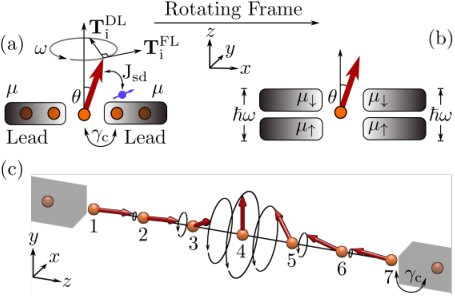
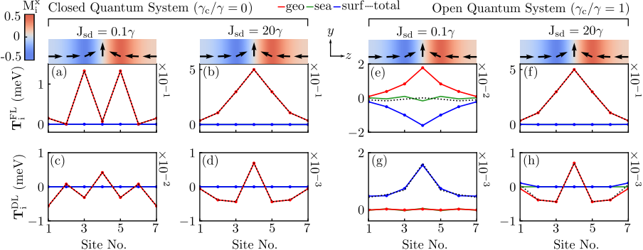
The STT vector, $\mathbf{T}=\mathbf{T}^{\mathrm{FL}}+\mathbf{T}^{\mathrm{DL}}$, can be decomposed [Fig. 1(a)] into: (i) even under time-reversal or field-like (FL) torque, which affects precession of LMM around $\mathbf{B}^{\rm eff}_{i}$; and (ii) odd under time-reversal or damping-like (DL) torque, which either enhances the Gilbert damping by pushing LMM toward $\mathbf{B}^{\rm eff}_{i}$ or competes with Gilbert term as “antidamping.” For example, negative values of $T^{\mathrm{DL}}=\mathbf{T}^{\mathrm{DL}}\cdot\mathbf{e}_{\mathrm{DL}}$ in Figs. 2 and  3, where $\mathbf{e}_{\mathrm{DL}}=(\mathbb{M}_{i}\times\partial\mathbb{M}_{i}/\partial t)|\mathbb{M}_{i}\times\partial\mathbb{M}_{i}/\partial t|^{-1}$, means that $\mathbf{T}^{\mathrm{DL}}$ vector points away from the axis of precession which is antidamping action. Similarly, $T^{\mathrm{FL}}=\mathbf{T}^{\mathrm{FL}}\cdot\mathbf{e}_{\mathrm{FL}}$, where $\mathbf{e}_{\mathrm{FL}}=(\partial\mathbb{M}_{i}/\partial t)|\partial\mathbb{M}_{i}/\partial t|^{-1}$, is plotted in Figs. 2 and  3.

The current-driven STT $\mathbf{T}_{i}\left[I^{S_{\alpha}}_{\mathrm{ext}}\right]$ acts as the counterpart of nonconservative force in nonadiabatic MD. The Gilbert damping plus current-independent torque $\mathbf{T}_{i}[\partial\mathbf{M}_{i}/\partial t]$ appear as the counterpart of electronic friction Bode2011; Thomas2012; Lu2012; Dou2018; Lu2019; Dou2017; Hopjan2018; Chen2019, but Gilbert damping requires agents Starikov2010 other than electrons alone considered in nonadiabatic MD. Thus, the geometric torque and damping, as counterparts of geometric magnetism force Berry1993 and friction Campisi2012, are absent from standard modeling of classical magnetization dynamics. Geometric torque has been added ad hoc into the LLG equation applied to specific problems, such as spin waves within bulk magnetic materials Wen1988; Niu1998; Niu1999. A recent study Stahl2017 of a single classical LMM embedded into a closed (i.e., finite length one-dimensional wire) electronic quantum system finds that nonequilibrium electronic spin density always generates geometric torque, even in perfectly adiabatic regime where electron-spin/LMM interaction is orders of magnitude larger than the characteristic frequency of LMM dynamics. It acts as a purely FL torque causing anomalous frequency of precession that is higher than the Larmor frequency. By retracing the same steps Thomas2012; Bode2011 in the derivation of the stochastic Langevin equation for electron-nuclei system connected to macroscopic reservoirs, Ref. Bode2012 derived the stochastic LLG equation Onoda2006; Nunez2008; Fransson2008; Hurst2020 for a single LMM embedded into an open electronic system out of equilibrium. The novelty in this derivation is damping, present even in the absence of traditional spin-flip relaxation mechanisms Zhang2004; Tatara2019, while the same conclusion about geometric torque changing only the precession frequency of LMM has been reached (in some regimes, geometric phase can also affect the stochastic torque Shnirman2015). However, single LMM is a rather special case, which is illustrated in Fig. 1(a) and revisited in Fig. 2, and the most intriguing situations in spintronics involve dynamics of noncollinear textures of LMMs. This is exemplified by current- or magnetic-field driven dynamics of domain walls (DWs) and skyrmions Tatara2019; Hurst2020; Petrovic2018; Bajpai2019a; Petrovic2019; Bostrom2019; Woo2017 where a much richer panoply of back-action effects from fast electronic system can be expected.

In this Letter, we analyze an exactly solvable model of seven steadily precessing LMMs, $\mathbf{M}_{1}(t)$–$\mathbf{M}_{7}(t)$ [Fig. 1(c)], which are noncollinear and noncoplanar and embedded into a one-dimensional (1D) infinite wire hosting conduction electrons. The model can be viewed as a segment of dynamical noncollinear magnetic texture, and it directly describes magnetic field-driven Woo2017 head-to-head Bloch DW McMichael1997 but without allowing it to propagate Woo2017; Petrovic2019. Its simplicity makes it exactly solvable—we fins the exact time-dependent DM via the nonequilibrium Green function (NEGF) formalism Stefanucci2013 and analyze its contributions in different regimes of the ratio $J_{sd}/\hbar\omega$ of $sd$ exchange interaction $J_{sd}$ Zhang2004 between electron spin and LMM and frequency of precession $\omega$. In both Figs. 1(a) and 1(c), the electronic subsystem is an open quantum system and, although no bias voltage is applied between the macroscopic reservoirs, it is pushed into the nonequilibrium state by the dynamics of LMMs. For example, electronic quantum Hamiltonian becomes time-dependent due to $\mathbf{M}_{1}(t)$ [Fig. 1(a)] or $\mathbf{M}_{1}(t)$–$\mathbf{M}_{7}(t)$ [Fig. 1(c)], which leads to pumping Tatara2019; Chen2009; Tserkovnyak2005 [Fig. 4(b),(c)] of spin current locally within the DW region, as well as into the leads [Fig. 4(a)]. Pumping of charge current will also occur if the left-right symmetry of the device is broken statically Chen2009 or dynamically Bajpai2019.

The electrons are modeled on an infinite tight-binding (TB) clean chain with Hamiltonian in the lab frame

Here $\hat{c}_{i}^{\dagger}=(\hat{c}_{i\uparrow}^{\dagger},\hat{c}_{i\downarrow}^{\dagger})$ and $\hat{c}_{i\sigma}^{\dagger}$ ($\hat{c}_{i\sigma}$) creates (annihilates) an electron of spin $\sigma=\uparrow,\downarrow$ at site $i$. The nearest-neighbor hopping $\gamma=1$ eV sets the unit of energy. The active region in Figs. 1(a) or  1(c) consists of one or seven sites, respectively, while the rest of infinite TB chain is taken into account as the left (L) and the right (R) semi-infinite leads described by the same Hamiltonian in Eq. (2), but with $J_{sd}=0$. The hopping between the leads and the active region is denoted by $\gamma_{c}$. The leads terminate at infinity into the macroscopic particle reservoirs with identical chemical potentials $\mu_{\mathrm{L}}=\mu_{\mathrm{R}}=E_{F}$ due to assumed absence of bias voltage, and $E_{F}=0$ is chosen as the Fermi energy. In contrast to traditional analysis in spintronics Zhang2004; Tatara2019, but akin to Refs. Stahl2017; Bode2012, Hamiltonian in Eq. (2) does not contain any spin-orbit or impurity terms as generators of spin-flip relaxation.

The spatial profile of Bloch DW is given by $M_{i}^{x}=-\sech[(h_{\mathrm{DW}}-z_{i})/W]\tanh[(Z_{\mathrm{DW}}-z_{i})]$, $M_{i}^{y}=\sech^{2}[(Z_{\mathrm{DW}}-z_{i})/W]$ and $M_{i}^{z}=\tanh[(Z_{\mathrm{DW}}-z_{i})/W]$, where $Z_{\mathrm{DW}}=4$ and $W=0.9$. Instead of solving LLG equations [Eq. (1)] for $\mathbb{M}_{1}(t)$–$\mathbb{M}_{7}(t)$, we impose a solution where LMMs precess steadily around the $z$-axis: $M_{i}^{x}(t)=\sin\theta_{i}\cos(\omega t+\phi_{i})$; $M_{i}^{y}(t)=\sin\theta_{i}\sin(\omega t+\phi_{i})$; and $M_{i}^{z}(t)=\cos\theta_{i}$. Using a unitary transformation into the rotating frame (RF), the Hamiltonian in Eq. (2) becomes time-independent Chen2009; Tatara2019, $\hat{H}_{\mathrm{RF}}=\hat{U}^{\dagger}(t)\hat{H}_{\mathrm{lab}}(t)\hat{U}(t)-i\hbar\hat{U}^{\dagger}\partial\hat{U}/\partial t=\hat{H}_{\mathrm{lab}}(t=0)-\hbar\omega\hat{\sigma}_{\alpha}/2$, with LMMs frozen at $t=0$ configuration from the lab. The unitary operator is $\hat{U}(t)=\exp(-i\omega t\hat{\sigma}_{\alpha}/2)$ for $\alpha$-axis of rotation. In the RF, the original two-terminal Landauer setup for quantum transport in Figs. 1(a) and  1(c) is mapped, due to $\hbar\omega\hat{\sigma}_{\alpha}/2$ term, onto an effective four-terminal setup Chen2009 [illustrated for single LMM in Fig. 1(b)]. Each of its four leads is an effective half-metal ferromagnet which accepts only one spin species, $\uparrow$ or $\downarrow$ along the $\alpha$-axis, and effective dc bias voltage $\hbar\omega/e$ acts between L or R pair of leads.

In the RF, the presence of the leads and macroscopic reservoirs can be taken into account exactly using steady-state NEGFs Stefanucci2013 which depend on time difference $t-t^{\prime}$ and energy $E$ upon Fourier transform. Using the retarded, $\hat{G}(E)$, and the lesser, $\hat{G}^{<}(E)$, Green functions (GFs), we find the exact nonequilibrium DM of electrons in the RF, $\hat{\rho}_{\mathrm{RF}}=\frac{1}{2\pi i}\int dE\,\hat{G}^{<}(E)$. Here the two GFs are related by the Keldysh equation, $\hat{G}^{<}(E)=\hat{G}(E)\hat{\Sigma}^{<}(E)\hat{G}^{\dagger}(E)$, where $\hat{\Sigma}^{<}(E)$ is the lesser self-energy Stefanucci2013 due to semi-infinite leads and $\hat{G}(E)=[E-\hat{H}_{\mathrm{RF}}-\hat{\Sigma}(E,\hbar\omega)]^{-1}$ with $\hat{\Sigma}(E,\hbar\omega)=\sum_{p=\mathrm{L,R},\sigma=\uparrow,\downarrow}\hat{\Sigma}_{p}^{\sigma}(E-Q_{\alpha}^{\sigma}\hbar\omega)$ being the sum of retarded self-energies for each of the four leads $p$, $\sigma$ in RF. We use shorthand notation $Q_{p}^{\uparrow}=-1/2$ and $Q_{p}^{\downarrow}=+1/2$. Since typical frequency of magnetization dynamics is $\hbar\omega\ll E_{F}$, we can expand Mahfouzi2013 $\hat{\rho}_{\mathrm{RF}}$ in small $\hbar\omega/E_{F}$ and then transform it back to the lab frame, $\hat{\rho}_{\mathrm{lab}}(t)=\hat{U}(t)\hat{\rho}_{\mathrm{RF}}\hat{U}^{\dagger}(t)$ to obtain $\hat{\rho}_{\mathrm{lab}}(t)=\hat{\rho}^{\mathrm{ad}}_{t}+\hat{\rho}_{\mathrm{geo}}(t)+\hat{\rho}_{\mathrm{sea}}(t)+\hat{\rho}_{\mathrm{surf}}(t)$ where:

We confirm by numerically exact calculations Petrovic2018 that thus obtained $\hat{\rho}_{\mathrm{lab}}(t)$ is identical to $\hbar G^{<}(t,t)/i$ computed in the lab frame. Here $\hat{G}_{0}(E)=[E-\hat{H}_{\mathrm{RF}}-\hat{\Sigma}(E,0)]^{-1}$ is $\hat{G}(E)$ with $\hbar\omega=0$; $\hat{\Gamma}_{p}^{\sigma}(E)=i[\hat{\Sigma}_{p}^{\sigma}(E)-\hat{\Sigma}^{\sigma}_{p}(E)^{\dagger}]$ is the level broadening matrix due the leads; and $f_{p}^{\sigma}(E)=f(E-[E_{F}+Q_{\alpha}^{\sigma}\hbar\omega])$ is the the Fermi function of macroscopic reservoir $p$, $\sigma$ in the RF.

The total nonequilibrium spin density, $\langle\hat{\mathbf{s}}_{i}\rangle(t)=\mathrm{Tr}[\hat{\rho}_{\mathrm{lab}}(t)|i\rangle\langle i|\otimes\hat{\bm{\sigma}}]=\langle\hat{\mathbf{s}}_{i}\rangle^{\mathrm{ad}}_{t}+\langle\hat{\mathbf{s}}_{i}\rangle_{\mathrm{geo}}(t)+\langle\hat{\mathbf{s}}_{i}\rangle_{\mathrm{sea}}(t)+\langle\hat{\mathbf{s}}_{i}\rangle_{\mathrm{surf}}(t)$, has the corresponding four contributions from DM contributions in Eq. (3). Here $\langle\hat{\mathbf{s}}_{i}\rangle^{\mathrm{ad}}_{t}$ is the equilibrium expectation value at an instantaneous time $t$ which defines ‘adiabatic spin density’ Zhang2004; Tatara2019; Niu1998; Niu1999; Stahl2017. It is computed using $\hat{\rho}^{\mathrm{ad}}_{t}$ as the grand canonical equilibrium DM expressed via the frozen (adiabatic) retarded GF Thomas2012; Bode2011; Bode2012, $\hat{G}_{t}(E)=[E-\hat{H}_{t}-\hat{\Sigma}]^{-1}$, for instantaneous configuration of $\mathbf{M}_{i}(t)$ while assuming $\partial\mathbf{M}_{i}/\partial t=0$ [subscript $t$ signifies parametric dependence on time through slow variation of $\mathbf{M}_{i}(t)$]. The other three contributions—from $\hat{\rho}_{\mathrm{geo}}(t)$ and $\hat{\rho}_{\mathrm{sea}}(t)$ governed by the Fermi sea and $\hat{\rho}_{\mathrm{surf}}(t)$ governed by the Fermi surface electronic states—contain first nonadiabatic correction Thomas2012; Bode2011; Bode2012 proportional to velocity $\partial\mathbf{M}_{i}/\partial t$, as well as higher order terms due to $\hat{\rho}_{\mathrm{lab}}(t)$ being exact. These three contributions define STT out of equilibrium Zhang2004; Petrovic2018; Mahfouzi2013

Each term $\mathbf{T}_{i}^{\mathrm{geo}}$, $\mathbf{T}_{i}^{\mathrm{sea}}$, $\mathbf{T}_{i}^{\mathrm{surf}}$ can be additionally separated into its own DL and FL components [Fig. 1(a)], as plotted in Figs. 2 and  3. Note that $\mathbf{T}_{i}^{\mathrm{sea}}$ is insignificant in both Figs. 2 and  3, so we focus on $\mathbf{T}_{i}^{\mathrm{geo}}$ and $\mathbf{T}_{i}^{\mathrm{surf}}$.

To gain transparent physical interpretation of $\mathbf{T}_{i}^{\mathrm{geo}}$ and $\mathbf{T}_{i}^{\mathrm{surf}}$, we first consider the simplest case Bode2012; Stahl2017—a single $\mathbf{M}_{1}(t)$ in setup of Fig. 1(a). The STT contributions as a function of the coupling $\gamma_{c}$ to the leads (i.e., reservoirs) are shown in Fig. 2. We use two different values for $J_{sd}$, where large ratio of $J_{sd}=20$ eV and $\hbar\omega=0.001$ eV is perfect adiabatic limit Niu1998; Niu1999; Stahl2017. Nevertheless, even in this limit and for $\gamma_{c}\rightarrow 0$ we find $\mathbf{T}_{1}^{\mathrm{geo}}\neq 0$ in Fig. 2(b) as the only nonzero and purely FL torque. This is also found in closed system of Ref. Stahl2017 where $\mathbf{T}_{1}^{\mathrm{geo}}$ was expressed in terms of the spin Berry curvature. As the quantum system becomes open for $\gamma_{c}>0$, $\mathbf{T}_{1}^{\mathrm{geo}}$ is slightly reduced while $\mathbf{T}_{1}^{\mathrm{surf}}$ emerges with small FL [Fig. 2(b)] and large DL [Fig. 2(d)] components. The DL torque $\mathbf{T}_{1}^{\mathrm{surf,DL}}$ points toward the $z$-axis and, therefore, enhances the Gilbert damping. In the wide-band approximation Bruch2016, the self-energy $\hat{\Sigma}(E)=-i\Gamma\hat{I}_{2}$ is energy-independent for $E$ within the bandwidth of the lead, which allows us to obtain analytical expression (at zero temperature)

Here $\mathbb{e}_{\phi}(t)=-\sin\omega t~\mathbb{e}_{x}+\cos\omega t~\mathbb{e}_{y}$. Thus, in perfect adiabatic limit, $J_{sd}/\hbar\omega\rightarrow\infty$, or in closed system, $\Gamma\rightarrow 0$, $\mathbf{T}_{1}^{\mathrm{geo}}$ is independent of microscopic parameters as expected from its geometric nature Wen1988. The always present $\mathbf{T}_{i}^{\mathrm{geo}}\neq 0$ means that electron spin is never along ‘adiabatic direction’ $\langle\hat{\mathbf{s}}_{i}\rangle^{\mathrm{ad}}_{t}$.

Switching to DW [Fig. 1(c)] embedded into a closed quantum system ($\gamma_{c}=0)$ shows in Fig. 3(a)–(d) that only $\mathbf{T}_{i}^{\mathrm{geo}}\neq 0$, which also acquires DL component locally with damping or antidamping action depending on the position of LMM. Upon opening the quantum system ($\gamma_{c}=\gamma$), Fig. 3(e)–(h) shows emergence of additional $\mathbf{T}^{\mathrm{surf}}_{i}\neq 0$ which, however, becomes negligible [Fig. 3(f),(h)] in the perfectly adiabatic limit $J_{sd}/\hbar\omega\gg 1$. At first sight, $\mathbf{T}_{i}^{\mathrm{geo,DL}}\neq 0$ violates Berry and Robbins original analysis Berry1993 according to which an isolated quantum system, with discrete energy spectrum, cannot exert friction onto the classical system. This apparent contradiction is resolved in Fig. 4(a) where we show that total $\sum_{i}\mathbf{T}_{i}^{\mathrm{geo,DL}}\equiv 0$ is always zero. Conversely, Fig. 4(a) confirms that total $\left(\sum\mathbf{T}^{\mathrm{surf,DL}}_{i}\right)_{z}\equiv I_{\mathrm{L}}^{S_{z}}+I_{\mathrm{R}}^{S_{z}}$ is identical to net spin current pumped into the leads via which the conduction electrons carry away excess angular momentum of precessing LMMs Tserkovnyak2005. Such identity underlies physical picture where spin current generated by time-dependent magnetization becomes DL torque Tserkovnyak2005; Zhang2009. Note that pumped spin current $I_{i\rightarrow j}^{S_{z}}$ due to $\hat{\rho}_{\mathrm{geo}}$ or $\hat{\rho}_{\mathrm{sea}}$ in Fig. 4(c) can be nonzero locally, but they sum to zero. The nonuniform pumped spin current due to spatially and time varying magnetization has prompted proposals Zhang2009; Kim2012 to amend the LLG equation by adding the corresponding DL torque $\mathbf{M}\times\mathcal{D}\cdot\partial\mathbf{M}/\partial t$ with $3\times 3$ damping tensor $\mathcal{D}$ whose spatial dependence is given by the so-called spin-motive force (SMF) formula. However, SMF correction was estimated to be small Kim2012 in the absence of spin-orbit coupling in the band structure. We confirm its smallness in Fig. 4(a),(b) for our DW case, but this actually reveals that SMF formula produces incorrectly an order of magnitude smaller torque than obtained from our exact $\hat{\rho}_{\mathrm{surf}}(t)$. Due to possibly complex Bajpai2019a time and spatial dependence of $\mathbf{T}_{i}^{\mathrm{surf}}$ and $\mathbf{T}_{i}^{\mathrm{geo}}$, the accurate path to incorporate them is offered by self-consistent coupling of electronic DM and LLG calculations, as proposed in Refs. Petrovic2018; Bostrom2019; Sayad2015 and in full analogy to how electronic friction is included in nonadiabatic MD Lu2019; Thomas2012; Bode2011; Lu2012; Dou2020; Dou2018; Dou2017; Hopjan2018; Chen2019.