Inflation with non-canonical scalar fields revisited
Abstract
We revisit inflation with non-canonical scalar fields by applying deformed-steepness exponential potentials. We show that the resulting scenario can lead to inflationary observables, and in particular to scalar spectral index and tensor-to-scalar ratio, in remarkable agreement with observations. Additionally, a significant advantage of the scenario is that the required parameter values, such as the non-canonicality exponent and scale, as well as the potential exponent and scale, do not need to acquire unnatural values and hence can accept a theoretical justification. Hence, we obtain a significant improvement with respect to alternative schemes, and we present distinct correlations between the model parameters that better fit the data, which can be tested in future probes. This combination of observational efficiency and theoretical justification makes the scenario at hand a good candidate for the description of inflation.
1 Introduction
Inflation is now a crucial part of the Standard Model of Cosmology [1, 2, 3, 4, 5]. Its solution to the horizon and flatness problems, together with the predictions for an almost scale invariant perturbation spectral index, have been confirmed by measurements of the cosmic microwave background (CMB) radiation. Nevertheless, the specific mechanism that triggers the inflationary epoch is one of the most outstanding issues in contemporary particle physics and cosmology. As a result, the building of theoretical models that explain this early accelerating expansion of the universe has exploded in recent years. The first main class of mechanisms that can lead to successful inflation is based on the introduction of a scalar field, while the second main class is obtained through gravitational modifications (for reviews see [6, 7, 8, 9, 10]). Consequently, inflation-related observations have provided significant insight to both modified gravity [11, 12, 13, 14, 15, 16], as well as to particle physics model building. The literature on the latter is very extensive, particularly within the framework of supersymmetry [17, 18, 19, 20], supergravity [21, 22, 23, 24], theories of extra dimensions such as superstring and brane theories [25, 26, 27], and technicolor too [28]. Detailed lists of references on different theoretical constructions can be found in [6, 7, 10].
In trying to understand the above issues (often in the framework of a single theory) several problems have been encountered, including fine-tuning issues (tiny dimensionless constants) and large predictions for tensor fluctuations. In this respect, theories of scalar fields with non-canonical kinetic terms, as expected in supergravity and superstring theories, including the -inflation subclass [29, 30, 31], were found to have significant advantages. These theories arise commonly in the framework of supergravity and string compactifications, which typically contain a large number of light scalar fields (moduli), whose dynamics are governed by a non-trivial moduli space metric . As long as the moduli space metric is not flat, we generically expect non-canonical kinetic terms. Such effects could, but need not, be suppressed by the high scale of the corresponding Ultra-Violet physics (e.g. moduli masses, string scale), but they can still have significant cosmological consequences through the dynamics of the dilaton and moduli fields.
Among their many advantages, non-canonical scalars satisfy in a more efficient way the slow-roll conditions of inflation, since the additional effective friction terms in the equations of motion of the inflaton slow down the scalar field for potentials which would otherwise be too steep. Hence, the resulting tensor-to-scalar ratio is significantly reduced [32, 33, 34, 35, 36, 37, 38, 39, 40, 41, 42, 43, 44, 45, 46, 47, 48, 49]. Moreover, models with non-canonical kinetic terms often allow for the kinetic term to play the role of dark matter and the potential terms to generate dark energy and inflation [50, 51, 52, 53]. Additionally, note that in the inflation realization in the context of Galileon and Horndeski theories, the role of the non-canonical kinetic term is also crucial [54, 55, 56, 57, 58, 59, 60]. The form of the non-canonical terms can vary significantly, since there are many plausible models, including different ways to achieve compactification. The recent cosmological data, however, together with the requirement to avoid fine-tuning and non-physical solutions, severely constrain the available possibilities.
On the other hand, an alternative way to improve the inflationary observables is by introducing an extra parameter as an exponent in the known potential forms, and thus affecting their steepness. In this way the dynamics of the scalar field can be additionally deformed, offering an alternative way to bring the tensor-to-scalar ratio to lower values without ruining the necessary spectral index [61, 62, 63, 64, 65, 66, 67, 68, 69, 70, 71].
One possible disadvantage of the above inflationary models, namely those with non-canonical terms and those with extra steepness parameter in the potential, is that the parameter values needed for acceptable observables are quite unnatural (with “natural” meaning the standard values of canonical kinetic term, no extra steepness parameter, and sub-Planckian potential values) and hard to be justified from the field-theoretical point of view. In particular, the non-canonical exponents need to be large, or the mass and potential parameters take trans-Planckian values. Hence, in this work, we are interested in studying a combination of the above models, specifically introducing a scalar field with non-canonical kinetic terms on top of a deformed-steepness potential with an extra parameter. As we will show, this enhances the range of solutions and leads to very satisfactory observables, for sets of model parameters significantly closer to the natural ones, that we proceed to identify and classify.
2 Non-canonical inflation with deformed-steepness potentials
In this section we present the scenario of non-canonical inflation with deformed-steepness potentials. We will focus on the usual non-canonical Lagrangian, which is well justified theoretically, and takes the form [29, 30, 31, 73, 72, 36],
| (2.1) |
where is the kinetic energy of the scalar field, and thus the action of the scenario reads
| (2.2) |
The parameter has dimensions of mass and determines the scale in which the non-canonical effects become significant, while is the Planck mass. Concerning the potential, in this work we will consider the deformed-steepness potential that was introduced in [61, 63], namely
| (2.3) |
with and the usual potential parameters and the new exponent parameter that determines the deformed-steepness.
We consider a homogeneous and isotropic flat Friedmann-Robertson-Walker (FRW) metric of the form
| (2.4) |
where is the scale factor. Variation of the action (2.2) in terms of the metric gives the following Friedmann equations
| (2.5) |
| (2.6) |
where is the Hubble parameter. Additionally, variation in terms of the scalar field leads to the Klein-Gordon equation
| (2.7) |
Note that one can write the above equation in the form of the usual conservation equation , using the definitions
| (2.8) |
In every inflationary scenario the important quantities are the inflation-related observables, namely the scalar spectral index of the curvature perturbations and its running , with the measure of the wave number , the tensor spectral index and its running, as well as the tensor-to-scalar ratio . In a given scenario these quantities depend on the model parameters, and hence confrontation with observational data can lead to constraints on these model parameters.
In order to extract the relations for the inflation-related observables, a detailed and thorough perturbation analysis is needed. In the simple case of canonical fields minimally coupled to gravity, and introducing the slow-roll parameters, full perturbation analysis indicates that the inflationary observables can be expressed solely in terms of the scalar potential and its derivatives [74, 7, 10]. However, in the case where non-canonical terms or forms of non-minimally coupling are present, as well as in the case where the potential itself is absent (as for instance in modified gravity inflation), one should instead introduce the Hubble slow-roll parameters (with positive integer), defined as [75, 76, 10, 77]
| (2.9) |
where is the e-folding number, and , where is the initial scale factor with the corresponding Hubble parameter (as usual inflation ends when ). Thus, the first three are found to be
| (2.10) | |||
| (2.11) | |||
| (2.12) |
With these definitions, the basic inflationary observables are given as [10]
| (2.13) | |||||
| (2.14) | |||||
| (2.15) | |||||
| (2.16) |
In the scenario of non-canonical inflation with deformed-steepness potentials, described by equations (2.5)-(2.7), the dynamics, i.e. the Hubble function, is determined by the parameters and related to “non-canonicality”, by the standard potential parameters and , alongside the deformed-steepness parameter . Hence, we deduce that the above inflationary observables (2.13)-(2.16) will be determined by these model parameters too. Nevertheless, we should mention that these parameters are not independent since they are related through the observed value of the amplitude of scalar perturbation . In particular, for the action (2.2) one finds [36]
| (2.19) |
which for our potential (2.3) leads to
| (2.20) |
with
| (2.21) |
Since we know that Planck observations give [78]
| (2.22) |
in the following analysis we set at will while arises from the satisfaction of the above observational constraint.
In the next section we investigate in detail the effect of each parameter on the inflationary observables, and we will show which combinations can bring the predictions deep inside the observational contours.
3 Results
In this section, we investigate the inflationary observables in the scenario of non-canonical inflation with deformed-steepness potentials. In particular, we desire to see how the scalar spectral index and the tensor-to-scalar ratio are affected by the model parameters. Since the involved equations (2.5)-(2.7), the slow-roll parameters (2.10)-(2.12) and the observables expressions (2.13)-(2.16) are in general too complicated to admit analytical solutions, we investigate them numerically.
Specifically, for a given set of parameter values we impose the conditions for , and corresponding to . According to (2.10)-(2.12), such suitably “small” imply and thus almost exponential expansion, which is the typical feature of inflation. We evolve the system and we determine the end of inflation by demanding at least one of the to become 1 (cases of eternal inflation, in which all remain smaller than 1 are considered non-physical), and thus by imposing the desired e-folding number we extract the time at the beginning of inflation. Hence, we can use the corresponding Hubble parameter to calculate the inflationary observables corresponding to the given parameter values and the imposed e-folding number .
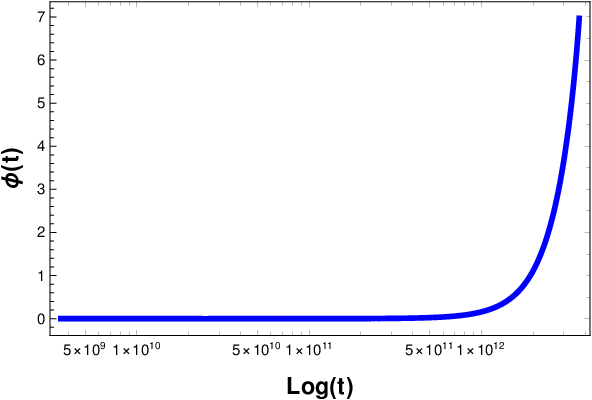
In order to show this in a more transparent way, in Fig. 1 we depict the evolution of , , and in terms of time. As we observe, initially and for a suitable time interval, are small and thus is almost constant, which indeed corresponds to inflation realization, while as time passes, increase and when one of them reaches 1 exponential expansion is not the case anymore ( decreases) and inflation ends. Hence, the imposed initial conditions have been chosen in order for a successful inflation to occur, which requires two conditions: i) the initial to be , and ii) before one of them reaches 1 and inflation ends to have obtained the required “suitable time interval”, namely expansion of 50-70 e-foldings. We mention that such background solutions are quite common for the studied range of the model parameters.



We start our investigation by examining the effect of the non-canonical parameter and the deformed-steepness parameter . Therefore, we fix and at theoretically motivated values and we calculate and for various combinations of and , adjusting suitably only the value of in order to satisfy the observational constraint (2.22), and for the e-folding number taking, as usual, the values 50, 60 and 70. In Table 1 we summarise the obtained observable predictions. Additionally, in order to present the information in a more transparent way that allows comparison with observational data, in Fig. 2 we depict the results of Table 1 on top of the 1 and 2 contours of the Planck 2018 data [78].
| , , | |||
|---|---|---|---|
| 50 | 60 | 70 | |
| 0.0445 | 0.0359 | 0.0299 | |
| 0.9670 | 0.9723 | 0.9761 | |
| , , | |||
|---|---|---|---|
| 50 | 60 | 70 | |
| 0.0341 | 0.0263 | 0.0209 | |
| 0.9649 | 0.9700 | 0.9736 | |
| , , | |||
|---|---|---|---|
| 50 | 60 | 70 | |
| 0.0240 | 0.0174 | 0.0130 | |
| 0.9611 | 0.9659 | 0.9693 | |
| , , | |||
|---|---|---|---|
| 50 | 60 | 70 | |
| 0.0350 | 0.0288 | 0.0244 | |
| 0.9670 | 0.9724 | 0.9763 | |
| , , | |||
|---|---|---|---|
| 50 | 60 | 70 | |
| 0.0318 | 0.0257 | 0.0214 | |
| 0.9666 | 0.9719 | 0.9758 | |
| , , | |||
|---|---|---|---|
| 50 | 60 | 70 | |
| 0.0282 | 0.0224 | 0.0183 | |
| 0.9657 | 0.9710 | 0.9748 | |
| , , | |||
|---|---|---|---|
| 50 | 60 | 70 | |
| 0.0289 | 0.0238 | 0.0202 | |
| 0.9668 | 0.9724 | 0.9762 | |
| , , | |||
|---|---|---|---|
| 50 | 60 | 70 | |
| 0.0268 | 0.0218 | 0.0183 | |
| 0.9660 | 0.9700 | 0.9759 | |
| , , | |||
|---|---|---|---|
| 50 | 60 | 70 | |
| 0.0245 | 0.0197 | 0.0163 | |
| 0.9653 | 0.9714 | 0.9746 | |


A general observation is that the predictions of the scenario at hand lie well inside the 1 region of the Planck 2018 data, without the need to use large values for the non-canonical parameter or the deformed-steepness parameter , which was indeed the main motivation behind the present work. Additionally, the predictions of the scenario are better, compared to the simple non-canonical models, as well as to the simple deformed-steepness models.
Concerning the specific features, we find the following: For any given set of model-parameters, increasing the e-folding values leads to increased and decreased , as is usual in the majority of inflationary scenarios. Now, for a given , as increases both and also increase. On the other hand, for a given , as increases there is no particular tendency for and . However, for larger , such as , the effect of is less significant and the different curves actually coincide. Moreover, as grows, slightly increases, while as grows slightly decreases.
We proceed by investigating the effect on the observables of the parameters and , which determine the scale of non-canonicality and of the potential, respectively, keeping in mind that the scale of inflation in theoretically motivated constructions can be anywhere from just below the unification scale (mostly Grand Unification), to energies as low as the scales within reach of the LHC (see e.g. [79]), with many possibilities in between, that can be linked i.e. to different stages of symmetry breaking. Without loss of generality we fix and and we calculate and for e-folding number being as usual 50, 60 and 70. We first additionally fix and change , and then we fix and change . In all cases we adjust the value of in order to satisfy the observational constraint (2.22). We summarise the obtained observable predictions in Table 2. Moreover, in order to present the results in a more transparent way, in Fig. 3 we depict the results of Table 2 on top of the 1 and 2 contours of the Planck 2018 data [78].
| , , | |||||||||
| 50 | 60 | 70 | 50 | 60 | 70 | 50 | 60 | 70 | |
| 0.0341 | 0.0263 | 0.0209 | 0.0475 | 0.0387 | 0.0325 | 0.0540 | 0.0447 | 0.0382 | |
| 0.9649 | 0.9700 | 0.9736 | 0.9674 | 0.9728 | 0.9766 | 0.9678 | 0.9732 | 0.9769 | |
| , , | |||||||||
| 50 | 60 | 70 | 50 | 60 | 70 | 50 | 60 | 70 | |
| 0.0341 | 0.0263 | 0.0209 | 0.0415 | 0.0332 | 0.0273 | 0.0504 | 0.0414 | 0.0351 | |
| 0.9649 | 0.9700 | 0.9736 | 0.9667 | 0.9720 | 0.9757 | 0.9678 | 0.9731 | 0.9769 | |


The main observation is that the predictions of the scenario lie well inside the 1 region of observational data. Now, for fixed , increasing leads to lower values of and ; moreover, the variation of is much faster than that of . Additionally, for fixed , increasing leads also to lower values of and ; nevertheless the change in is strongly affected by the change in (since appears in powers of four in the equations) that it can easily be led outside the observational contours. This similar tendency behavior was expected, since in the scalar-field equation (2.7) the two parameters and appear multiplied. Nevertheless, this is not a trivial result, since is related to the non-canonicality scale while to the potential scale.
From the above analysis we deduce that non-canonical kinetic terms combined with deformed-steepness potentials can provide inflationary predictions in very good agreement with observations, compared to simple non-canonical models [32, 33, 34, 35, 36, 37, 38, 39, 40, 41, 42, 43, 44, 45, 46, 47, 48, 49] as well as to canonical models with deformed-steepness potentials [61, 62, 63, 64, 65, 66, 67, 68]. An additional significant advantage is that the above combination allows to achieve good predictions without the need to use unnaturally large values for or , or unnaturally tuned values for the non-canonicality and potential scales and , as well as for the potential exponent . In particular, we see that and remain in reasonable sub-Planckian regions, with values that can be easily predicted and accepted from field theoretical point of view. This combination of observational efficiency and theoretical justification is a significant advantage of the scenario at hand.
4 Conclusions
In this work we revisited inflation with non-canonical scalar fields by applying deformed-steepness exponential potentials. Non-canonical kinetic terms can arise straightforwardly in models of supergravity and superstrings, while exponential potentials have remarkable properties, as they greatly facilitate slow roll and result to scaling behaviour at large scales.
As we have shown, the resulting scenario can lead to inflationary observables, and in particular to scalar spectral index of the curvature perturbations and tensor-to-scalar ratio , in remarkable agreement with the observations of Planck 2018, being well inside the 1 region. Apart from observational predictability, a significant additional advantage of the proposed scenario arises from the theoretical point of view. In particular, in order to obtain acceptable observables, in simple non-canonical models one needs to use relatively large non-canonical exponent or ranges of values for the non-canonicality scale , while in canonical models with deformed-steepness potentials relatively large values of the extra exponent need to be imposed, and, hence, these models cannot be well-justified theoretically. On the other hand, in the scenario of the present work the exponents and are small, as well as the non-canonicality and potential scales and remain in reasonable sub-Planckian regions.
We mention here that the motivation for the deformed-steepness parameter of [63] was the improved inflationary observables (specifically ) compared to the simplest slow-roll models. Moreover, the motivation for the extra parameter compared to canonical models is to also improve . Nevertheless, in works with non-minimal kinetic terms but with no deformed-steepness parameter () the improvement of the observables is obtained for very large values (of the order of 100 or 1000 [36]). Hence, the motivation for allowing both and is to be able to obtain improved observables, but with very low, and thus closer to natural, . Although the scenario has extra parameters, the improvement in observables (smaller tensor-to-scalar ratio values), as well as the higher naturalness is worth the price.
Our analysis revealed that, for a given , as increases both and decrease too, while on the other hand, for a given , as increases there is no particular tendency for and . Additionally, for fixed , increasing leads to lower values of and , while for fixed , increasing leads to lower values of and too.
In summary, we showed that revisiting non-canonical inflation models by applying potentials with deformed steepness, increases the observational predictability, bringing the scalar spectral index and the tensor-to-scalar ratio more deeply into the observational contours, offering a better theoretical justification for the required parameters. This combination of observational efficiency and theoretical justification is a significant advantage of the scenario at hand, and hence, non-canonical models with deformed-steepness potential need to be further explored, as additional observational data will be coming forward.
References
- [1] A. A. Starobinsky, A New Type of Isotropic Cosmological Models Without Singularity, Phys. Lett. B 91, 99 (1980).
- [2] D. Kazanas, Dynamics of the Universe and Spontaneous Symmetry Breaking, Astrophys. J. Lett. 241, L59-L63 (1980).
- [3] K. Sato, First Order Phase Transition of a Vacuum and Expansion of the Universe, Mon. Not. Roy. Astron. Soc. 195, 467 (1981).
- [4] A. H. Guth, The Inflationary Universe: A Possible Solution to the Horizon and Flatness Problems, Phys. Rev. D 23, 347 (1981).
- [5] A. D. Linde, A New Inflationary Universe Scenario: A Possible Solution of the Horizon, Flatness, Homogeneity, Isotropy and Primordial Monopole Problems, Phys. Lett. B 108, 389 (1982).
- [6] K. A. Olive, Inflation, Phys. Rept. 190, 307 (1990).
- [7] D. H. Lyth and A. Riotto, Particle physics models of inflation and the cosmological density perturbation, Phys. Rept. 314, 1 (1999) [arXiv:hep-ph/9807278].
- [8] N. Bartolo, E. Komatsu, S. Matarrese and A. Riotto, Non-Gaussianity from inflation: Theory and observations, Phys. Rept. 402, 103 (2004) [arXiv:astro-ph/0406398].
- [9] S. Nojiri and S. D. Odintsov, Unified cosmic history in modified gravity: from F(R) theory to Lorentz non-invariant models, Phys. Rept. 505, 59 (2011) [arXiv:1011.0544].
- [10] J. Martin, C. Ringeval and V. Vennin, Encyclopaedia Inflationaris, Phys. Dark Univ. 5-6, 75-235 (2014) [arXiv:1303.3787].
- [11] Stephen A. Appleby, Richard A. Battye, Alexei A. Starobinsky, Curing singularities in cosmological evolution of F(R) gravity, JCAP 06, 005 (2010) [arXiv:astro-ph.CO/0909.1737].
- [12] S. Nojiri and S. D. Odintsov, Modified gravity with negative and positive powers of the curvature: Unification of the inflation and of the cosmic acceleration, Phys. Rev. D 68, 123512 (2003) [arXiv:hep-th/030728].
- [13] B. M. Carter and I. P. Neupane, Towards inflation and dark energy cosmologies from modified Gauss-Bonnet theory, JCAP 06, 004 (2006) [arXiv:hep-th/0512262].
- [14] R. Ferraro and F. Fiorini, Modified teleparallel gravity: Inflation without inflaton, Phys. Rev. D 75, 084031 (2007) [arXiv:gr-qc/0610067].
- [15] C. Germani and A. Kehagias, New Model of Inflation with Non-minimal Derivative Coupling of Standard Model Higgs Boson to Gravity, Phys. Rev. Lett. 105, 011302 (2010) [arXiv:1003.2635].
- [16] L. Sebastiani, G. Cognola, R. Myrzakulov, S. Odintsov and S. Zerbini, Nearly Starobinsky inflation from modified gravity, Phys. Rev. D 89, no.2, 023518 (2014) [arXiv:1311.0744].
- [17] Ellis, John R. and Nanopoulos, Dimitri V. and Olive, Keith A. and Tamvakis, K., Cosmological Inflation Cries Out for Supersymmetry, Phys. Lett. B 118, 335-339 (1982).
- [18] J.R. Ellis, A.D. Linde and D.V. Nanopoulos, Inflation Can Save the Gravitino, Phys.Lett. B 118, 59-64 (1982).
- [19] G.R. Dvali, Q. Shafi, R.K. Schaefer, Large scale structure and supersymmetric inflation without fine tuning, Phys.Rev.Lett. 73, 1886-1889 (1994) [arXiv:hep-ph/9406319].
- [20] G.G. Ross and S. Sarkar, Successful supersymmetric inflation, Nucl. Phys. B 461, 597-624 (1996) [arXiv:hep-ph/9506283].
- [21] D.V. Nanopoulos, K. A. Olive, M. Srednicki and K. Tamvakis, Primordial Inflation in Simple Supergravity, Phys.Lett. B 123, 41-44 (1983).
- [22] Ewan D. Stewart, Inflation, supergravity and superstrings, Phys.Rev. D 51, 6847-6853 (1995) [arXiv:hep-ph/9405389].
- [23] Edi Halyo, Hybrid inflation from supergravity D-terms, Phys.Lett. B 387, 43-47 (1996) [arXiv:hep-ph/9606423].
- [24] Andrei D. Linde, Antonio Riotto, Hybrid inflation in supergravity, Phys.Rev. D 56, 1841-1844 (1997) [arXiv:hep-ph/9703209].
- [25] Q. Shafi, C. Wetterich, Inflation From Higher Dimensions, Nucl.Phys. B 289, 787-809 (1987).
- [26] Ignatios Antoniadis, C. Bachas, John R. Ellis, Dimitri V. Nanopoulos, Cosmological String Theories and Discrete Inflation, Phys.Lett. B 211, 393-399 (1988).
- [27] G.R. Dvali, S.H.Henry Tye, Brane inflation, Phys.Lett. B 450, 72-82 (1999) [arXiv:hep-ph/9812483].
- [28] Fred C. Adams et al., Natural inflation: Particle physics models, power law spectra for large scale structure, and constraints from COBE, Phys.Lett. D 47, 426-455 (1993) [arXiv:hep-ph/9207245].
- [29] C. Armendariz-Picon, T. Damour and V. F. Mukhanov, k - inflation, Phys. Lett. B 458, 209-218 (1999) [arXiv:hep-th/9904075].
- [30] J. Garriga and V. F. Mukhanov, Perturbations in k-inflation, Phys. Lett. B 458, 219-225 (1999) [arXiv:hep-th/9904176].
- [31] V. F. Mukhanov and A. Vikman, Enhancing the tensor-to-scalar ratio in simple inflation, JCAP 02, 004 (2006) [arXiv:astro-ph/0512066].
- [32] G. Barenboim and W. H. Kinney, Slow roll in simple non-canonical inflation, JCAP 03, 014 (2007) [arXiv:astro-ph/0701343].
- [33] K. Tzirakis and W. H. Kinney, Non-canonical generalizations of slow-roll inflation models, JCAP 01, 028 (2009) [arXiv:0810.0270].
- [34] P. Franche, R. Gwyn, B. Underwood and A. Wissanji, Attractive Lagrangians for Non-Canonical Inflation, Phys. Rev. D 81, 123526 (2010) [arXiv:0912.1857].
- [35] P. Franche, R. Gwyn, B. Underwood and A. Wissanji, Initial Conditions for Non-Canonical Inflation, Phys. Rev. D 82, 063528 (2010) [arXiv:1002.2639].
- [36] S. Unnikrishnan, V. Sahni and A. Toporensky, Refining inflation using non-canonical scalars, JCAP 08, 018 (2012) [arXiv:1205.0786].
- [37] R. Gwyn, M. Rummel and A. Westphal, Relations between canonical and non-canonical inflation, JCAP 12, 010 (2013) [arXiv:1212.4135].
- [38] D. A. Easson and B. A. Powell, The Degeneracy Problem in Non-Canonical Inflation, JCAP 03, 028 (2013) [arXiv:1212.4154].
- [39] X. M. Zhang and j. Y. Zhu, Extension of warm inflation to noncanonical scalar fields, Phys. Rev. D 90, no.12, 123519 (2014) [arXiv:1402.0205].
- [40] R. Gwyn and J. L. Lehners, Non-Canonical Inflation in Supergravity, JHEP 05, 050 (2014) [arXiv:1402.5120].
- [41] M. W. Hossain, R. Myrzakulov, M. Sami and E. N. Saridakis, Variable gravity: A suitable framework for quintessential inflation, Phys. Rev. D 90, no.2, 023512 (2014) [arXiv:1402.6661].
- [42] K. Rezazadeh, K. Karami and P. Karimi, Intermediate inflation from a non-canonical scalar field, JCAP 09, 053 (2015) [arXiv:1411.7302].
- [43] S. Cespedes and A. C. Davis, Non-canonical inflation coupled to matter, JCAP 11, 014 (2015) [arXiv:1506.01244].
- [44] N. K. Stein and W. H. Kinney, Planck Limits on Non-canonical Generalizations of Large-field Inflation Models, JCAP 04, 006 (2017) [arXiv:1609.08959].
- [45] K. Dimopoulos and C. Owen, Quintessential Inflation with -attractors, JCAP 06, 027 (2017) [arXiv:1703.00305].
- [46] A. Mohammadi, K. Saaidi and H. Sheikhahmadi, Constant-roll approach to non-canonical inflation, Phys. Rev. D 100, no.8, 083520 (2019) [arXiv:1803.01715].
- [47] M. Naderi, A. Aghamohammadi, A. Refaei and H. Sheikhahmadi, Intermediate inflation with non-canonical scalar field in the low anisotropy Universe, Mod. Phys. Lett. A 34, no.33, 1950272 (2019) [arXiv:1809.02348].
- [48] A. Y. Kamenshchik, A. Tronconi, T. Vardanyan and G. Venturi, Non-Canonical Inflation and Primordial Black Holes Production, Phys. Lett. B 791, 201-205 (2019) [arXiv:1812.02547].
- [49] T. Q. Do, W. Kao and I. C. Lin, CMB imprints of non-canonical anisotropic inflation, [arXiv:2003.04266].
- [50] N. Bose and A. Majumdar, A k-essence Model Of Inflation, Dark Matter and Dark Energy, Phys. Rev. D 79, 103517 (2009) [arXiv:0812.4131].
- [51] J. De-Santiago and J. L. Cervantes-Cota, Generalizing a Unified Model of Dark Matter, Dark Energy, and Inflation with Non Canonical Kinetic Term, Phys. Rev. D 83, 063502 (2011) [arXiv:1102.1777].
- [52] V. Sahni and A. A. Sen, A new recipe for CDM, Eur. Phys. J. C 77, no.4, 225 (2017) [arXiv:1510.09010].
- [53] S. S. Mishra and V. Sahni, Unifying Dark Matter and Dark Energy with non-Canonical Scalars, [arXiv:1803.09767].
- [54] T. Kobayashi, M. Yamaguchi and J. Yokoyama, G-inflation: Inflation driven by the Galileon field, Phys. Rev. Lett. 105, 231302 (2010) [arXiv:1008.0603].
- [55] C. Burrage, C. de Rham, D. Seery and A. J. Tolley, Galileon inflation, JCAP 01, 014 (2011) [arXiv:1009.2497].
- [56] J. Ohashi and S. Tsujikawa, Potential-driven Galileon inflation, JCAP 10, 035 (2012) [arXiv:1207.4879].
- [57] S. Tsujikawa, The effective field theory of inflation/dark energy and the Horndeski theory, Lect. Notes Phys. 892, 97-136 (2015) [arXiv:1404.2684].
- [58] Alexei A. Starobinsky, Sergey V. Sushkov, Mikhail S. Volkov, The screening Horndeski cosmologies, JCAP 06, 007 (2016) [arXiv:1604.06085].
- [59] L. Sebastiani, S. Myrzakul and R. Myrzakulov, Reconstruction of k-essence inflation in Horndeski gravity, Eur. Phys. J. Plus 132, no.10, 433 (2017) [arXiv:1702.00064].
- [60] G. Koutsoumbas, K. Ntrekis, E. Papantonopoulos and E. N. Saridakis, Unification of Dark Matter - Dark Energy in Generalized Galileon Theories, JCAP 02, 003 (2018) [arXiv:1704.08640].
- [61] C. Q. Geng, M. W. Hossain, R. Myrzakulov, M. Sami and E. N. Saridakis, Quintessential inflation with canonical and noncanonical scalar fields and Planck 2015 results, Phys. Rev. D 92, no.2, 023522 (2015) [arXiv:1502.03597].
- [62] K. Rezazadeh, K. Karami and S. Hashemi, Tachyon inflation with steep potentials, Phys. Rev. D 95, no.10, 103506 (2017) [arXiv:1508.04760].
- [63] C. Q. Geng, C. C. Lee, M. Sami, E. N. Saridakis and A. A. Starobinsky, Observational constraints on successful model of quintessential Inflation, JCAP 06, 011 (2017) [arXiv:1705.01329].
- [64] S. Ahmad, R. Myrzakulov and M. Sami, Relic gravitational waves from Quintessential Inflation, Phys. Rev. D 96, no.6, 063515 (2017) [arXiv:1705.02133].
- [65] A. Agarwal, R. Myrzakulov, M. Sami and N. K. Singh, Quintessential inflation in a thawing realization, Phys. Lett. B 770, 200-208 (2017) [arXiv:1708.00156].
- [66] M. Skugoreva, M. Sami and N. Jaman, Emergence of cosmological scaling behavior in the asymptotic regime, Phys. Rev. D 100, no.4, 043512 (2019) [arXiv:1901.06036].
- [67] S. Das, M. Banerjee and N. Roy, Dynamical System Analysis for Steep Potentials, JCAP 08, 024 (2019) [arXiv:1903.02288].
- [68] G. B. Lima and R. O. Ramos, Unified early and late Universe cosmology through dissipative effects in steep quintessential inflation potential models, Phys. Rev. D 100, no.12, 123529 (2019) [arXiv:1910.05185].
- [69] S. Nojiri, S.D. Odintsov, V.K. Oikonomou, Modified Gravity Theories on a Nutshell: Inflation, Bounce and Late-time Evolution, Phys.Rept. 692 1-104,(2017) [arXiv:1705.11098].
- [70] Sukannya Bhattacharya, Mayukh R. Gangopadhyay, Study in the noncanonical domain of Goldstone inflation, Phys.Rev.D 101, no.2, 023509,(2020) [arXiv:1812.08141].
- [71] Sukannya Bhattacharya, Mayukh R. Gangopadhyay, Indrani Banerjee, Sumanta Chakraborty, Soumitra SenGupta, Phys.Rev.D 99, no.2, 023515,(2019) [arXiv:1806.11327].
- [72] S. Li and A. R. Liddle, Observational constraints on K-inflation models, JCAP 10, 011 (2012) [arXiv:1204.6214].
- [73] S. Unnikrishnan, Can cosmological observations uniquely determine the nature of dark energy ?, Phys. Rev. D 78, 063007 (2008) [arXiv:0805.0578].
- [74] J. E. Lidsey, A. R. Liddle, E. W. Kolb, E. J. Copeland, T. Barreiro and M. Abney, Reconstructing the inflation potential : An overview, Rev. Mod. Phys. 69, 373 (1997) [arXiv:astro-ph/9508078].
- [75] D. I. Kaiser, Primordial spectral indices from generalized Einstein theories, Phys. Rev. D 52, 4295 (1995) [arXiv:astro-ph/9408044].
- [76] M. Sasaki and E. D. Stewart, A General analytic formula for the spectral index of the density perturbations produced during inflation, Prog. Theor. Phys. 95, 71 (1996) [arXiv:astro-ph/9507001].
- [77] R. P. Woodard, Perturbative Quantum Gravity Comes of Age, Int. J. Mod. Phys. D 23, no. 09, 1430020 (2014) [arXiv:1407.4748].
- [78] Y. Akrami et al. [Planck Collaboration], Planck 2018 results. X. Constraints on inflation, [arXiv:1807.06211].
- [79] G. German, A. de la Macorra and M. Mondragon, Low scale supergravity inflation with R symmetry, Phys. Lett. B 494, 311-317 (2000) [arXiv:hep-th/0006200].