Inflation and Reheating in theory formulated in the Palatini formalism
Abstract
A new model for inflation using modified gravity in the Palatini formalism is constructed. Here non-minimal coupling of scalar field with the curvature as a general function is considered. Explicit inflation models for some choices of are developed. By writing an equivalent scalar-tensor action for this model and going over to Einstein frame, slow roll parameters are constructed. There exists a large parameter space for different choices of and potentials which satisfy values of and limits on compatible with Planck 2018 data. Further, we calculate reheating temperature and the number of e-folds at the end of reheating for different values of equation of state parameter for all the constructed models.
1 Introduction
There are mainly two formulations in General Relativity (GR) popularly known as Palatini and Metric formalisms. Palatini formalism or first order formalism treats space-time connections as independent variable[1, 2, 3, 4, 5, 6, 7, 8, 9], whereas in Metric formalism, these connections are not independent but derived from the metric itself. But in GR these two approaches produce same Einstein equation. Hence dynamics are equivalent in both formalisms. This is not true for modified gravity models and models where fields are nonminimally coupled to gravity. In these cases, both formalisms represent different physical situations [1, 2, 3].
Inflation [10, 11, 12, 13, 14, 15, 16] was first developed in the early 1980s to solve problems of standard Big Bang theory like horizon problem, fine-tuning problem etc. Quantum fluctuations also started during the period of inflation which led to the cosmic microwave background(CMB) anisotropy and provided the seed for the formation of large scale structure of the universe. A more popular model for inflation is the Starobinsky model which is a pure gravity theory with an additional term in the Einstein-Hilbert action. An equivalent scalar-tensor theory of Starobinsky model has an additional scalar degree of freedom apart from two tensor degrees of freedom of Einstein-Hilbert action[17, 18, 19]. In Einstein frame, this theory is equivalent to the usual scalar field model with a potential suitable for a valid inflation model which satisfies all the constraints from CMB data.
In a broad sense, the Starobinsky model falls under a general framework of f(R) gravity. The above analysis works best in metric formulation of gravity. However, in the Palatini formalism, no additional propagating degrees of freedom appears in f(R) gravity theory [3]. Because of this, no inflation is possible in this scenario. Hence a scalar field needs to be added to this action to develop an Inflation model in Palatini formulation of gravity. In this line, first work appeared in [20] where nonminimal couplings of scalars are considered. Since then many works related to different inflationary potentials, preheating, reheating, postinflationary phases, dark matter has been done with many variants of action including a term [21, 22, 23, 24, 25, 26, 27, 28, 29, 30, 31, 32, 33, 34, 35, 36, 37, 38, 39, 40, 41, 42, 43, 44, 45, 46, 47, 48, 49, 50, 51, 52, 53, 54, 55, 56, 57, 58, 59, 60, 61, 62, 63, 64, 65, 66]. For an introduction to Palatini inflation models refer to [67] and references therein.
In this work, we formulate a palatini inflation model in theory. In metric formalism inflation model in gravity has been considered earlier in literature [68, 69, 70]. Recently, it has been shown that the appearance of terms like in the one loop effective action for massless, conformally coupled scalar field [71]. Our action is of the form similar to form obtained in [68]. But our approach here is to develop a model of inflation in palatini formalism. We show that such an action provide a favorable inflationary scenario satisfying Planck 2018 data [72].
Reheating [73, 74, 75, 76] is a phenomenon which acts as a transit between Inflation and the radiation dominated era of the universe. There are various models on how the inflaton field loses its energy. Using techniques similar to [77, 78, 79, 80, 81], the number of e-folds and temperature at the end of reheating ( and ) can be written in terms of inflationary observables. Earlier, reheating in Palatini models of inflation has been discussed in these papers. [57, 45, 59]
This paper is organized as follows. In the next section, we introduce the action of our model. Then we express it in terms of equivalent scalar-tensor action in Einstein frame. In section 3, slow roll parameters are defined. Values of and are also calculated numerically and the results are presented. Section 4 is dedicated to the calculations of reheating parameters. At last, in section 5, we summarize our results.
2 The Model
We start with a general action of the form -
| (2.1) |
where is the metric, is its determinant, , is the Ricci scalar defined as in Palatini formalism and is a constant. Here we have chosen Planck mass to be unity. An equivalent action in terms of an auxiliary field can be written as -
| (2.2) |
where . Varying with respect to in equation (2.2), we get if and using this result in equation (2.2), we recover equation (2.1). Rearranging equation (2.2), the action becomes -
| (2.3) |
where . By making a conformal transformation -
| (2.4) |
action is obtained in Einstein frame as -
| (2.5) |
Let us define a new potential as -
| (2.6) |
Now for our choice of [68], the new potential can be written as -
| (2.7) |
Varying equation (2.5) with respect to , we get the constraint equation -
| (2.8) |
Inserting equation (2.8) to equation (2.7), we can eliminate . Then again inserting equation (2.7) to equation (2.5) and rearranging and simplifying, we get -
| (2.9) |
Now the last term can be defined as effective potential in the Einstein frame -
| (2.10) |
In order to bring kinetic part of scalar field into that of canonical form, we introduce a new field as -
| (2.11) |
In terms of , equation (2.9) becomes -
| (2.12) |
Now we are ready to build up our inflation model, with this action. Next, we define the slow-roll parameters to estimate the observables which will decide the fate of our model. Here we have neglected contribution due to the third term of the action to the inflation phase. This is a valid assumption so far as the slow-roll inflation is concerned (see [67] and references therein). In this case then, it is a model of inflation driven by a scalar field with potential 11 1 Background evolution of field for a flat FRW metric with scale factor and hubble parameter is- (2.13) where and and ′ represent derivatives with respect to conformal time and respectively. Under slow-roll approximation, terms proportional to and can be neglected and equation (2.13) reduces to usual FRW equations for minimally coupled field. .
3 Slow-roll parameters and Results
Before analyzing the dynamics of our model, we define slow-roll parameters (mainly and ) which are helpful to decide whether a model can describe inflation or not. They can be written as -
| (3.1) |
The slow roll parameters and must be during inflation phase of expansion. For the potential in equation (2.10), slow roll parameters become -
| (3.2) | |||||
where and are slow-roll parameters for and ′ represents derivative with respect to . Number of e-folds from the time when a mode crosses the horizon to the end of inflation, can be written as (for unit Planck mass) -
| (3.3) |
Inflation ends when and this, in turn, determines the value of . Putting the value of and (taken in between 60 and 70) in (3.3) , value of can be obtained. Putting this value to equations (3) and (3), value of and can be obtained respectively. Scalar spectral index and tensor-to-scalar ratio can then be calculated from the following equations -
| (3.4) |
Now we estimate and for various cases. Here we restrict our analysis only for quadratic and quartic potentials. We choose two values of and and is a dimensionless constant.
Case 1 : and
For this case -
| (3.5) |
As neither nor depend on , so it will lead to constant and for a particular choice of , and . In this case, then it would be difficult to end the inflation and to decide the value of . Therefore we will not discuss this case further here.
Case 2 : and
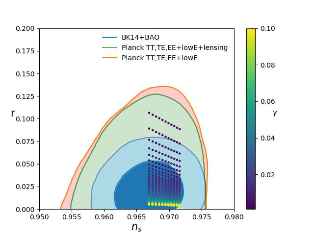
In this case, and depend only on h and for a particular value of . The parameters and fixes the value of the field or In fig. 3, potential vs is plotted. In fig. 3 the relation between vs is plotted. The value of changes discontinuously as changes from negative to positive value. Here positive sign is taken in equation (2.11). Instead if negative sign is taken, all values of ’s will be negative. However, discontinuity of is there for both positive and negative sign. For fig. 3 and fig. 3, the value of parameters , and is chosen. For this particular set, the numerically estimated value of and are and respectively(we take here). Also the result for spectral index and tensor to scalar ratio is shown in fig. 3. Here is changing and , and negative sign is considered in equation (2.11). It clearly shows that there can be large parameter space available which can satisfy Planck constraints.


Case 3 : and
For case 3 and case 4, is taken as . This makes the Lagrangian in (2.1) equivalent to the form plus usual scalar field term. Similar to case 2, the graphs of vs and vs are shown in fig 7 and fig. 7 respectively. Unlike to the previous case, here is continuous for all range of . For fig 7 and fig 7, the value of parameters are , and For this particular value of parameters, we obtain and . The potential in equation (2.10) takes the form -
| (3.6) |
Dividing both numerator and denominator by , we get -
| (3.7) |
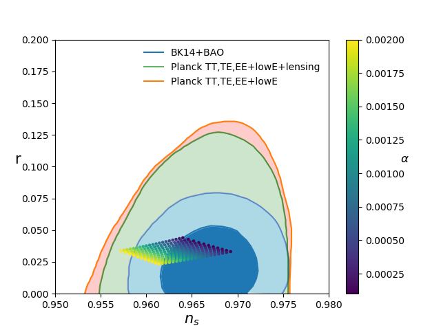
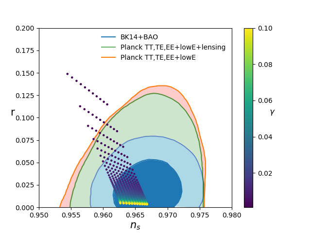
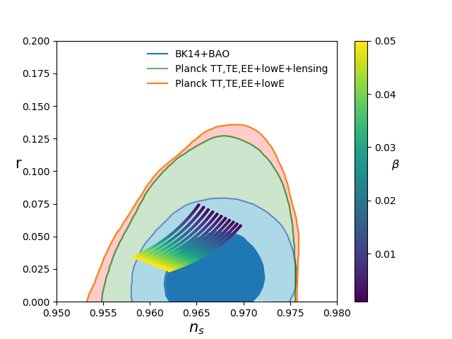
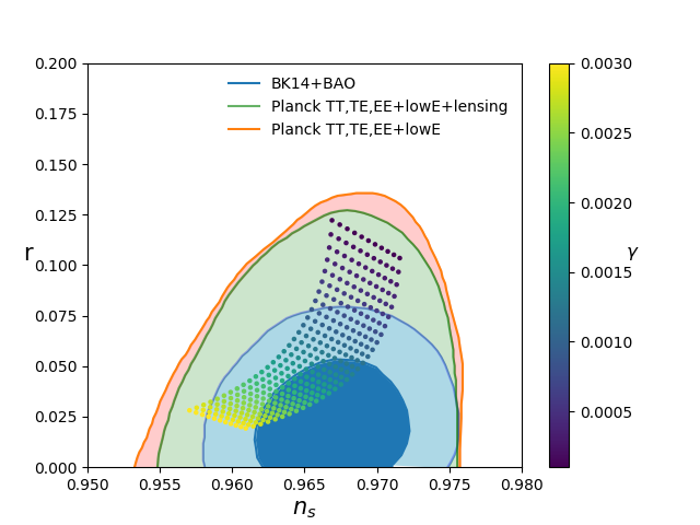
We can clearly observe that as . Hence this potential will not give rise to plateau unlike the results for Lagrangian where is coupled only with [38, 39, 40, 82, 45, 49]. The results for and are shown in fig. 7, 7 and 8. In fig. 7, , and is changing. In fig. 7, , and is changing. And in fig. 8, , and is changing. Here we consider positive sign in equation (2.11). Note that both 7 and 7 look same. This happens because in the expression of and , and always appear in pairs i.e. in the form of or . Similar to case 2, here also a large parameter space available which satisfies Planck constraints on and It is observed from 8 that we can tune the parameters of our model to obtain a very small value for



Case 4 : and
Analogous to case 3, potential graph and vs are shown in fig 10 and fig 10 for , and which give and . Here, potential in equation (2.10) becomes -
| (3.8) |
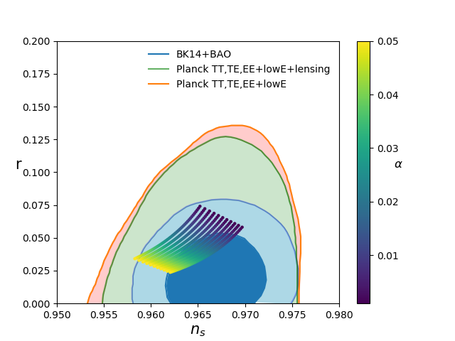
As , . So again no plateau in the potential. The and graphs are plotted in fig. 12, 12 and 13. In fig. 12 , and is changing. In fig. 12 , and is varying. In fig. 13 , and is varying. Here we consider positive sign in equation (2.11). In this case as well, we find a large parameter space available which is compatible with Planck 2018 data.


4 Reheating
In this section our aim is to find the reheating temperature, and number of e-folds at the end of reheating, for our models. Equation of state during reheating is parameterised by a function , which is obtained from -
| (4.1) |
where and represent pressure and density of a particular component. For radiation and matter dominated universe, the value of is and respectively. Here we consider ranging from to during reheating period [79]. We also assume that is constant throughout the reheating period. Mathematically, the number of e-folds at the end of reheating is defined as -
| (4.2) |
where denotes scale factor at the end of reheating and denotes scale factor at the end of inflation. Using continuity equation along with and assuming conservation of energy, one can derive the following equations [79]-
| (4.3) |
| (4.4) |
Here denotes pivot scale of horizon crossing, denotes the potential at the end of inflation, and denotes the number of relativistic species at the end of reheating. Note that in equation (4.3), as increases, decreases. Hence more instant reheating implies more temperature. For , we can not extract any information of from equation (4.4) as both RHS and LHS get canceled out. This happens because when , the boundary between reheating period and the radiation dominated era is indistinguishable. For , equation (4.4) becomes -
| (4.5) |
For , equation (4.4) writes as-
| (4.6) |
| (4.7) |
| (4.8) |
Until now, we have done the model independent calculations. Now we are ready to do the model dependent calculations for our cases except case .
Case 2 : and
For this case, equation (3.3) provides (considering sign before term) -
| (4.9) |
Assuming , we get . Also and for this case is written as-
| (4.10) |
| (4.11) |
Using the above relations, we obtain-
| (4.12) |
| (4.13) |
| (4.14) |
Also can be written as -
| (4.15) |
Equations (4.7) and (4.8) can be expressed in terms of inflationary observable parameter using the above relations. Figure 14 is obtained by varying from to for , and . Here we use . The shaded blue region corresponds to Planck’s value and the shaded red region is obtained from the fact that Big Bang nucleosynthesis temperature should not be less than . All lines meet when which means that instantaneous reheating occurs irrespective of the choices of . Also, the temperature is maximum for instantaneous reheating as expected. For , as any value of would satisfy equation (4.5), hence it will give rise to a vertical line passing through instantaneous reheating point. The graph shows good agreement with Planck’s data for all values of .

Case 3 : and
For case 3, can not be expressed in terms of in a simplified form. Hence we need to take some approximation. Note that in fig. 7, we have taken , and which are favourable by Planck data. Also value is of the . Hence, in the equation (3.6), we can safely neglect term in comparison to and . With this approximation, , , and become -
| (4.16) |
| (4.17) |
| (4.18) |
Using the above expressions, we obtain the following equations -
| (4.19) |
| (4.20) |
| (4.21) |
Substituting , and into equation (4.7) and equation (4.8) and varying from to , we plot and vs in the figure 16. Here we have taken , and . These are the same values using which we obtained figures 7 and 7. It is observed that all values give rise to reheating parameters within known bound. If we change by an order of , we did not find any substantial change in value. This can be seen from figure 16, here is set to and , has same value as in figure 16.

to . Here red, blue, green and orange colour
lines correspond to and
respectively.

to . Here red, blue, green and orange colour
lines correspond to and
respectively.
Case 4 : and
Similar to the case 3, here also we need to take a simplified form of by taking appropriate approximation. Taking hint from the values in figures 10 and 10, along with the fact that value of is of , we can neglect the term in comparison to and in equation (3.8). With this approximation, , and become -
| (4.22) |
| (4.23) |
| (4.24) |
Using these equations, we obtain the following relations -
| (4.25) |
| (4.26) |
| (4.27) |
Now we are ready to obtain and as a function of .

5 Conclusion
Inflation models are constructed in a modified gravity theory in Palatini formalism. Here our modified action contains a general non-minimal coupling of scalar field with and term separately. Unlike metric formalism, Palatini formalism does not introduce a new scalar degree of freedom in our theory. It turns out that term in the action can be translated to a higher order kinetic term and a new potential term for scalar field in an equivalent scalar-tensor set-up in Einstein frame. However, in slow-roll inflation setting we can safely neglect the effect of higher order kinetic term in the action. The modified potential is responsible for the inflation. In this equivalent scalar-tensor theory, we calculate scalar spectral index and tensor to scalar ratio() for four different cases depending on the form of nonminimal coupling and potential of scalar field. We have varied three unknown parameters of our theory to extract the information about and It is observed that in most of the cases we have a large parameter space which can match with the results of Planck 2018 constraints on and Palatini formalism in modified gravity theories may provide a large class of models for Inflation satisfying CMB data. We have studied reheating phenomenon for the models considered in this paper which are compatible with Planck data. Also a more general action with nonminimal coupling of scalar field can be studied to explore the cosmology of very early universe. A dark energy picture of these models is worth investing in future.
Acknowledgments
This work was partially funded by DST (Govt. of India), Grant No. SERB/PHY/2017041.
References
- [1] T. P. Sotiriou, f(R) gravity and scalar-tensor theory, Class. Quant. Grav. 23 (2006) 5117–5128, [gr-qc/0604028].
- [2] T. P. Sotiriou and S. Liberati, Metric-affine f(R) theories of gravity, Annals Phys. 322 (2007) 935–966, [gr-qc/0604006].
- [3] T. P. Sotiriou and V. Faraoni, f(R) Theories Of Gravity, Rev. Mod. Phys. 82 (2010) 451–497, [0805.1726].
- [4] M. Borunda, B. Janssen and M. Bastero-Gil, Palatini versus metric formulation in higher curvature gravity, JCAP 11 (2008) 008, [0804.4440].
- [5] A. De Felice and S. Tsujikawa, f(R) theories, Living Rev. Rel. 13 (2010) 3, [1002.4928].
- [6] G. J. Olmo, Palatini Approach to Modified Gravity: f(R) Theories and Beyond, Int. J. Mod. Phys. D 20 (2011) 413–462, [1101.3864].
- [7] S. Capozziello and M. De Laurentis, Extended Theories of Gravity, Phys. Rept. 509 (2011) 167–321, [1108.6266].
- [8] T. Clifton, P. G. Ferreira, A. Padilla and C. Skordis, Modified Gravity and Cosmology, Phys. Rept. 513 (2012) 1–189, [1106.2476].
- [9] S. Nojiri, S. Odintsov and V. Oikonomou, Modified Gravity Theories on a Nutshell: Inflation, Bounce and Late-time Evolution, Phys. Rept. 692 (2017) 1–104, [1705.11098].
- [10] A. H. Guth, Inflationary universe: A possible solution to the horizon and flatness problems, Phys. Rev. D 23 (Jan, 1981) 347–356.
- [11] A. Starobinsky, A new type of isotropic cosmological models without singularity, Physics Letters B 91 (1980) 99 – 102.
- [12] A. Linde, A new inflationary universe scenario: A possible solution of the horizon, flatness, homogeneity, isotropy and primordial monopole problems, Physics Letters B 108 (1982) 389 – 393.
- [13] A. Linde, Chaotic inflation, Physics Letters B 129 (1983) 177 – 181.
- [14] D. H. Lyth and A. Riotto, Particle physics models of inflation and the cosmological density perturbation, Phys. Rept. 314 (1999) 1–146, [hep-ph/9807278].
- [15] A. Riotto, Inflation and the theory of cosmological perturbations, ICTP Lect. Notes Ser. 14 (2003) 317–413, [hep-ph/0210162].
- [16] D. Baumann, Inflation, in Physics of the large and the small, TASI 09, proceedings of the Theoretical Advanced Study Institute in Elementary Particle Physics, Boulder, Colorado, USA, 1-26 June 2009, pp. 523–686, 2011, 0907.5424, DOI.
- [17] A. A. Starobinsky, A New Type of Isotropic Cosmological Models Without Singularity, Adv. Ser. Astrophys. Cosmol. 3 (1987) 130–133.
- [18] V. F. Mukhanov and G. V. Chibisov, Quantum Fluctuations and a Nonsingular Universe, JETP Lett. 33 (1981) 532–535.
- [19] A. A. Starobinsky, The Perturbation Spectrum Evolving from a Nonsingular Initially De-Sitter Cosmology and the Microwave Background Anisotropy, Sov. Astron. Lett. 9 (1983) 302.
- [20] F. Bauer and D. A. Demir, Inflation with Non-Minimal Coupling: Metric versus Palatini Formulations, Phys. Lett. B 665 (2008) 222–226, [0803.2664].
- [21] T. Koivisto and H. Kurki-Suonio, Cosmological perturbations in the palatini formulation of modified gravity, Class. Quant. Grav. 23 (2006) 2355–2369, [astro-ph/0509422].
- [22] N. Tamanini and C. R. Contaldi, Inflationary Perturbations in Palatini Generalised Gravity, Phys. Rev. D 83 (2011) 044018, [1010.0689].
- [23] F. Bauer and D. A. Demir, Higgs-Palatini Inflation and Unitarity, Phys. Lett. B 698 (2011) 425–429, [1012.2900].
- [24] K. Enqvist, T. Koivisto and G. Rigopoulos, Non-metric chaotic inflation, JCAP 05 (2012) 023, [1107.3739].
- [25] A. Borowiec, M. Kamionka, A. Kurek and M. Szydlowski, Cosmic acceleration from modified gravity with Palatini formalism, JCAP 02 (2012) 027, [1109.3420].
- [26] A. Stachowski, M. Szydł owski and A. Borowiec, Starobinsky cosmological model in Palatini formalism, Eur. Phys. J. C 77 (2017) 406, [1608.03196].
- [27] C. Fu, P. Wu and H. Yu, Inflationary dynamics and preheating of the nonminimally coupled inflaton field in the metric and Palatini formalisms, Phys. Rev. D 96 (2017) 103542, [1801.04089].
- [28] S. Rasanen and P. Wahlman, Higgs inflation with loop corrections in the Palatini formulation, JCAP 11 (2017) 047, [1709.07853].
- [29] T. Tenkanen, Resurrecting Quadratic Inflation with a non-minimal coupling to gravity, JCAP 12 (2017) 001, [1710.02758].
- [30] A. Racioppi, Coleman-Weinberg linear inflation: metric vs. Palatini formulation, JCAP 12 (2017) 041, [1710.04853].
- [31] T. Markkanen, T. Tenkanen, V. Vaskonen and H. Veermäe, Quantum corrections to quartic inflation with a non-minimal coupling: metric vs. Palatini, JCAP 03 (2018) 029, [1712.04874].
- [32] L. Järv, A. Racioppi and T. Tenkanen, Palatini side of inflationary attractors, Phys. Rev. D 97 (2018) 083513, [1712.08471].
- [33] S. Rasanen, Higgs inflation in the Palatini formulation with kinetic terms for the metric, 1811.09514.
- [34] A. Racioppi, New universal attractor in nonminimally coupled gravity: Linear inflation, Phys. Rev. D 97 (2018) 123514, [1801.08810].
- [35] P. Carrilho, D. Mulryne, J. Ronayne and T. Tenkanen, Attractor Behaviour in Multifield Inflation, JCAP 06 (2018) 032, [1804.10489].
- [36] V.-M. Enckell, K. Enqvist, S. Rasanen and E. Tomberg, Higgs inflation at the hilltop, JCAP 06 (2018) 005, [1802.09299].
- [37] F. Bombacigno and G. Montani, Big bounce cosmology for Palatini gravity with a Nieh–Yan term, Eur. Phys. J. C 79 (2019) 405, [1809.07563].
- [38] V.-M. Enckell, K. Enqvist, S. Rasanen and L.-P. Wahlman, Inflation with term in the Palatini formalism, JCAP 1902 (2019) 022, [1810.05536].
- [39] I. Antoniadis, A. Karam, A. Lykkas and K. Tamvakis, Palatini inflation in models with an term, JCAP 11 (2018) 028, [1810.10418].
- [40] I. Antoniadis, A. Karam, A. Lykkas, T. Pappas and K. Tamvakis, Rescuing Quartic and Natural Inflation in the Palatini Formalism, JCAP 03 (2019) 005, [1812.00847].
- [41] S. Rasanen and E. Tomberg, Planck scale black hole dark matter from Higgs inflation, JCAP 01 (2019) 038, [1810.12608].
- [42] J. P. B. Almeida, N. Bernal, J. Rubio and T. Tenkanen, Hidden Inflaton Dark Matter, JCAP 03 (2019) 012, [1811.09640].
- [43] T. Takahashi and T. Tenkanen, Towards distinguishing variants of non-minimal inflation, JCAP 04 (2019) 035, [1812.08492].
- [44] K. Kannike, A. Kubarski, L. Marzola and A. Racioppi, A minimal model of inflation and dark radiation, Phys. Lett. B 792 (2019) 74–80, [1810.12689].
- [45] T. Tenkanen, Minimal Higgs inflation with an term in Palatini gravity, Phys. Rev. D 99 (2019) 063528, [1901.01794].
- [46] K. Shimada, K. Aoki and K.-i. Maeda, Metric-affine Gravity and Inflation, Phys. Rev. D 99 (2019) 104020, [1812.03420].
- [47] J. Wu, G. Li, T. Harko and S.-D. Liang, Palatini formulation of gravity theory, and its cosmological implications, Eur. Phys. J. C 78 (2018) 430, [1805.07419].
- [48] A. Kozak and A. Borowiec, Palatini frames in scalar–tensor theories of gravity, Eur. Phys. J. C 79 (2019) 335, [1808.05598].
- [49] R. Jinno, K. Kaneta, K.-y. Oda and S. C. Park, Hillclimbing inflation in metric and Palatini formulations, Phys. Lett. B 791 (2019) 396–402, [1812.11077].
- [50] A. Edery and Y. Nakayama, Palatini formulation of pure gravity yields Einstein gravity with no massless scalar, Phys. Rev. D 99 (2019) 124018, [1902.07876].
- [51] J. Rubio and E. S. Tomberg, Preheating in Palatini Higgs inflation, JCAP 04 (2019) 021, [1902.10148].
- [52] R. Jinno, M. Kubota, K.-y. Oda and S. C. Park, Higgs inflation in metric and Palatini formalisms: Required suppression of higher dimensional operators, JCAP 03 (2020) 063, [1904.05699].
- [53] M. Giovannini, Post-inflationary phases stiffer than radiation and Palatini formulation, Class. Quant. Grav. 36 (2019) 235017, [1905.06182].
- [54] T. Tenkanen and L. Visinelli, Axion dark matter from Higgs inflation with an intermediate , JCAP 08 (2019) 033, [1906.11837].
- [55] N. Bostan, Quadratic, Higgs and hilltop potentials in the Palatini gravity, 1908.09674.
- [56] T. Tenkanen, Trans-Planckian censorship, inflation, and dark matter, Phys. Rev. D 101 (2020) 063517, [1910.00521].
- [57] I. D. Gialamas and A. Lahanas, Reheating in Palatini inflationary models, Phys. Rev. D 101 (2020) 084007, [1911.11513].
- [58] M. Shaposhnikov, A. Shkerin and S. Zell, Quantum Effects in Palatini Higgs Inflation, 2002.07105.
- [59] A. Lloyd-Stubbs and J. McDonald, Sub-Planckian Inflation in the Palatini Formulation of Gravity with an term, 2002.08324.
- [60] P. M. Sá, Unified description of dark energy and dark matter within the generalized hybrid metric-Palatini theory of gravity, 2002.09446.
- [61] I. Antoniadis, A. Lykkas and K. Tamvakis, Constant-roll in the Palatini- models, JCAP 04 (2020) 033, [2002.12681].
- [62] D. Ghilencea, Palatini quadratic gravity: spontaneous breaking of gauged scale symmetry and inflation, 2003.08516.
- [63] T. Takahashi, T. Tenkanen and S. Yokoyama, Violation of slow-roll in non-minimal inflation, 2003.10203.
- [64] A. Racioppi, Non-Minimal (Self-)Running Inflation: Metric vs. Palatini Formulation, 1912.10038.
- [65] D. D. Canko, I. D. Gialamas and G. P. Kodaxis, A simple deformation of Starobinsky inflationary model, Eur. Phys. J. C 80 (2020) 458, [1901.06296].
- [66] R. Myrzakulov, L. Sebastiani and S. Vagnozzi, Inflation in -theories and mimetic gravity scenario, Eur. Phys. J. C 75 (2015) 444, [1504.07984].
- [67] T. Tenkanen, Tracing the high energy theory of gravity: an introduction to Palatini inflation, Gen. Rel. Grav. 52 (2020) 33, [2001.10135].
- [68] T. Rador, f(R) Gravities a la Brans-Dicke, Phys. Lett. B 652 (2007) 228–232, [hep-th/0702081].
- [69] A. de la Cruz-Dombriz, E. Elizalde, S. D. Odintsov and D. Sáez-Gómez, Spotting deviations from R2 inflation, JCAP 05 (2016) 060, [1603.05537].
- [70] J. Mathew, J. P. Johnson and S. Shankaranarayanan, Inflation with in Jordan frame, Gen. Rel. Grav. 50 (2018) 90, [1705.07945].
- [71] D. Glavan, S. Miao, T. Prokopec and R. Woodard, One-loop Graviton Corrections to Conformal Scalars on de Sitter, 2007.10395.
- [72] Planck collaboration, N. Aghanim et al., Planck 2018 results. VI. Cosmological parameters, 1807.06209.
- [73] D. Boyanovsky, H. de Vega and R. Holman, Erice lectures on inflationary reheating, in International School of Astrophysics, D. Chalonge: 5th Course: Current Topics in Astrofundamental Physics, pp. 183–270, 9, 1996, hep-ph/9701304.
- [74] B. A. Bassett, S. Tsujikawa and D. Wands, Inflation dynamics and reheating, Rev. Mod. Phys. 78 (2006) 537–589, [astro-ph/0507632].
- [75] R. Allahverdi, R. Brandenberger, F.-Y. Cyr-Racine and A. Mazumdar, Reheating in Inflationary Cosmology: Theory and Applications, Ann. Rev. Nucl. Part. Sci. 60 (2010) 27–51, [1001.2600].
- [76] M. A. Amin, M. P. Hertzberg, D. I. Kaiser and J. Karouby, Nonperturbative Dynamics Of Reheating After Inflation: A Review, Int. J. Mod. Phys. D 24 (2014) 1530003, [1410.3808].
- [77] L. Dai, M. Kamionkowski and J. Wang, Reheating constraints to inflationary models, Phys. Rev. Lett. 113 (2014) 041302, [1404.6704].
- [78] J. B. Munoz and M. Kamionkowski, Equation-of-State Parameter for Reheating, Phys. Rev. D 91 (2015) 043521, [1412.0656].
- [79] J. L. Cook, E. Dimastrogiovanni, D. A. Easson and L. M. Krauss, Reheating predictions in single field inflation, JCAP 04 (2015) 047, [1502.04673].
- [80] M. Drewes, J. U. Kang and U. R. Mun, CMB constraints on the inflaton couplings and reheating temperature in -attractor inflation, JHEP 11 (2017) 072, [1708.01197].
- [81] A. Nautiyal, Reheating constraints on Tachyon Inflation, Phys. Rev. D 98 (2018) 103531, [1806.03081].
- [82] T. Tenkanen and E. Tomberg, Initial conditions for plateau inflation: a case study, JCAP 04 (2020) 050, [2002.02420].