Kinetic theory for spin-1/2 particles in ultra-strong magnetic fields

Quantum kinetic descriptions of plasmas are typically of most interest for high densities and modest temperature Haas 2011. For this purpose, typically the the starting point is the Wigner-Moyal equation Haas 2011; Shukla and Eliasson 2011; Daligault 2014; Materdey and Seyler 2003; Yang and Yao 1991; Misra et al. 2017, or various generalizations thereof also accounting for physics associated with the electron spin, such as the magnetic dipole force Zamanian et al. 2010a; Andreev 2017, spin magnetization Zamanian et al. 2010a; Andreev and Trukhanova 2018 and spin-orbit interaction Andreev and Trukhanova 2018. Both weakly Asenjo et al. 2012; Manfredi et al. 2019 and strongly Ekman et al. 2017; Ekman et al. 2019 relativistic treatments have been presented in the recent literature.

Certain quantum phenomena depend strongly on the magnitude of the electromagnetic field, however, rather than on the density and temperature parameters. Phenomena such as radiation reaction (reviewed in, e.g., Ref. Burton and Noble 2014) and pair-creation fall into this category.¹¹ 1 While the classical radiation reaction, where the response is a smooth function of the orbit, is a useful approximation as long as the emitted spectrum is soft (dominated by photons with energies well below $mc^{2}$), the description based on QED (see e.g. Ilderton and Torgrimsson 2013; Cole et al. 2018), containing discrete probabilistic contributions due to the emission of high energy quanta, is more generally applicable. Another field-dependent phenomenon is Landau quantization Eliezer et al. 2005, which becomes prominent whenever the Zeeman energy due to the magnetic field is comparable to or larger than the thermal energy, or the Fermi energy, in the case of degenerate electrons.

In the atmospheres of pulsars and magnetars Harding and Lai 2006, the electron motion may become relativistic, and the magnetic field strength can be ultra-strong, i.e., the Zeeman energy may be comparable to or even larger than the electron rest mass energy Uzdensky and Rightley 2014. Further information about pulsar properties can be gained through the emission profiles, see, e.g., Refs Stinebring et al. 1984; Rankin 1990; Han et al. 1998. Theoretical studies of wave propagation relevant for strongly magnetized objects have been made both with kinetic Melrose and Weise 2009 and hydrodynamic Asenjo et al. 2011; Zamanian et al. 2010b models. However, most previous theoretical studies starting from the Dirac equation (see also Ekman et al. 2017; Manfredi et al. 2019) have been limited to cases where the magnetic field strength is well below the critical field $B_{cr}=m^{2}c^{2}/\left|q\right|\hbar$.

Our objective in this work is to derive a fully relativistic kinetic model of spin-1/2 particles, applicable for ultra-strong magnetic fields, i.e. with

relaxing the conditions given in previous works. Assuming that the electric field is low enough to avoid pair creation (i.e., below the critical electric field $E_{cr}=m^{2}c^{3}/\left|q\right|\hbar$), we can use the Foldy-Wouthuysen transformation Foldy and Wouthuysen 1950; Silenko 2008 to separate particle states from antiparticle states in the Dirac equation. Moreover, we limit ourselves to the case where the characteristic spatial scale length of the fields is much longer than the Compton length $L_{c}=\hbar/mc$.

Making a Wigner transformation of the density matrix, our approach results in an evolution equation for a $2\times 2$ Wigner matrix, where the four components encode information regarding the spin states. However, the off-diagonal elements of the matrix is associated with the spin-precession dynamics which is too rapid to be resolved by the theory. Thus a further reduction is made, where only the diagonal components representing the spin-up and the spin-down states relative to the magnetic field remain.

Together with Maxwell’s equations, we obtain a closed system describing the plasma dynamics. A novel feature of the model is the energy expression, where the usual gamma factor from classical relativistic theory is replaced by an operator in phase space, also depending on the magnetic field. Interestingly, the Landau-quantized states in a constant magnetic field turn out to be eigenfunctions of the energy-operator of this theory, which is helpful when computing the thermodynamic background state for the Wigner matrix. To demonstrate the usefulness of the theory, we compute the dispersion relation for Langmuir waves propagating parallel to an external magnetic field. Finally, the consequences of the theory and applications to astrophysics are discussed

To derive our theory for ultra-strong magnetic fields, we will take the Dirac Hamiltonian

as our starting point. Here $m$ is the mass, $\hat{\mathcal{E}}=q\phi(\hat{\mathbf{r}})$, and $\hat{\mathcal{O}}=\bm{\alpha}\cdot\hat{\bm{\pi}}$, and $\bm{\alpha}$ and $\beta$ are the Dirac matrices. Furthermore $\hat{\mathbf{p}}$ is the canonical momentum, $\hat{\bm{\pi}}=\hat{\mathbf{p}}-q\mathbf{A}(\hat{\mathbf{r}},t)$, $q$ is the charge, and $\phi$ and $\mathbf{A}$ are, respectively, the scalar and vector potentials. From now one we use units such that $c=1$.

In their seminal paper Foldy and Wouthuysen Foldy and Wouthuysen 1950 found a way to decouple the upper and lower two components of the four-spinor. For the general case, this can be done up to a given order in a suitably chosen expansion parameter. In Ref. Foldy and Wouthuysen 1950 this parameter was $1/m$, meaning that the expansion is valid for sufficiently small energies. In this paper we will use the results of Refs. Silenko 2003; Silenko 2008 where a modified Foldy-Wouthuysen transformation was developed for the case where the expansion parameter is instead the scale-length of the fields. This transformation hence makes it possible to take into account arbitrarily strong fields as long as we are only concerned with variations on sufficiently long scale-lengths.

The goal of a Foldy-Wouthuysen transformation is to obtain a Hamiltonian where the upper and lower pairs of components of the four-spinor are decoupled in the regime of interest. An operator is called odd if it couples the upper and the lower pairs of components of the four-spinor, and even if it does not. The odd and even terms of the Hamiltonian Eq. 2 are $\hat{\mathcal{E}}$ and $\hat{\mathcal{O}}$, respectively, satisfying $[\beta,\hat{\mathcal{E}}]=0$ and $\{\beta,\hat{\mathcal{O}}\}=0$.

In Silenko 2003, Silenko found a unitary transformation of the Hamiltonian operator

where

where $\hat{\epsilon}=\sqrt{m^{2}+\hat{\mathcal{O}}^{2}}$. Furthermore, using the Dirac Hamiltonian $\hat{H}$ in Eq. 3, one obtains

where

where $\hat{T}=\sqrt{2\hat{\epsilon}(m+\hat{\epsilon})}$ and $\hat{\mathcal{F}}=\hat{\mathcal{E}}-i\hbar\partial_{t}$. The Hamiltonian $H^{\prime}$ still has odd terms, the anti-commutators in $\hat{\mathcal{O}}^{\prime}$ are linear in $\hat{\mathcal{O}}$, i.e. linear in $\bm{\alpha}$. However, the odd term $\hat{\mathcal{O}}^{\prime}$ in $H^{\prime}$ should be small compared to $\hat{\epsilon}$, after choosing an expansion parameter. Since we are interested in the effects of an ultra-strong magnetic field, our small expansion parameters will be the electric field strength $E/E_{\text{cr}}$(such that pair production is negligible) and the inverse scale-length of the fields $L_{c}/L$, but we will make no assumption on the magnetic field strength.

Thus a second transformation can be preformed with the following operator

Since $\hat{\mathcal{O}}^{\prime}$ is small, only the major corrections are taken into account. Finally, the transformed Hamiltonian is

This Hamiltonian has no odd terms, so we are done with the transformation of the Dirac Hamiltonian. Until now, we have presented the Foldy-Wouthuysen transformation derived in Ref. Silenko 2008. Our approach now is to calculate the commutators occurring in Eq. 5 to all orders in the magnetic field. In doing this we will expand some of them in a series using Ref. Transtrum and Van Huele 2005, see the Appendix for more details. After the calculation, the Hamiltonian $H^{\prime}$ in Eq. 5 becomes

where

where $\mu_{B}=q\hbar/2m$ is the Bohr magneton and

Note that we kept all orders of the magnetic field. However we only kept up to first order of the combination of $\hbar$ with $E$ and $\nabla_{r}$. In the expression for $\hat{H}^{\prime}$ there are still some odd operators, but since $\hat{\mathcal{O}}^{\prime}$ is linear in $\mu_{B}E$ and $\mu_{B}\partial_{t}B$, they should be smaller than $\hat{\epsilon}$. Thus it is fine to only include the minor correction of the second transformation in Eq. 7. Thus the Hamiltonian $\hat{H}_{FW}$ after the second transformation will have the same structure as in Eq. 8. However, the anti-commutator in $\hat{H}_{FW}$ in Eq. 8 is proportional to the square of $\hat{\mathcal{O}}^{\prime}$. Since we only kept up to first order of $E$ and $\partial_{t}B$, we keep only the first two terms of $\hat{H}_{FW}$

where $\hat{\epsilon}=\sqrt{m^{2}+\hat{\bm{\pi}}^{2}-2\mu_{B}m\hat{\bm{\Sigma}}\cdot\mathbf{B}}$. Taking the limit of weak $B$-field, i.e. keeping up to first order in $\mu_{B}B/m$, we recover the Hamiltonian in Silenko 2008. The Hamiltonian in Eq. 12 includes the spin orbit interaction, see Ekman et al. 2017 for more details, but since $E\ll B$, it is negligible compared to the magnetic interaction. We will therefore neglect the spin-orbit interaction from now on, as the main idea of this paper is to study the effects of a strong magnetic field on the dynamics of a plasma. The transformed Hamiltonian is now

This Hamiltonian includes all orders of $\mu_{B}B/m$ and is fully relativistic, hence is suitable to be used in deriving a kinetic equation for plasma in an environment where the magnetic field is of the order of the critical field $B_{\text{cr}}$. Note that all operators in both Eq. 12 and Eq. 13 are even, thus we will let $\beta\rightarrow 1$ and $\hat{\bm{\Sigma}}\rightarrow\bm{\sigma}$ from now on.

Now we want to derive a kinetic equation using the Hamiltonian Eq. 13. To do that, we start with the evolution equation for the density matrix $\hat{\rho}_{\alpha\beta}$ which is given by the Von Neumann equation

Our goal now is to transform this equation into a kinetic equation for the Wigner quasi-distribution function. Considering the gauge-invariant Wigner function derived by Stratonovich Stratonovich 1956

We express Eq. 14 in terms of $\rho(\mathbf{r},\mathbf{r}^{\prime})$ and use the identities Stratonovich 1956

These identities can be utilized for a function $F$ that only depends on $\hat{\bm{\pi}}$. However, our Hamiltonian in Eq. 13 depends on both $\mathbf{B}(\hat{\mathbf{r}})$ and $\hat{\bm{\pi}}$, thus we divide the magnetic field as

where $\mathbf{B}_{0}$ is a constant strong magnetic field and $\delta\mathbf{B}(\hat{\mathbf{r}})$ is a varying magnetic field. Furthermore, a Taylor series around $\mathbf{B}=\mathbf{B}_{0}$ can be done, see Ref. Kumar 1965 for more details. However, the Taylor series gets more complicated for the higher order terms, thus a restriction on $\delta\mathbf{B}(\hat{\mathbf{r}})$ needs to be done. Considering the case where $\mu_{B}\delta B/m\ll 1$, note that we did consider $\mu_{B}E/m\ll 1$ in the previous section, the Hamiltonian becomes

While this Hamiltonian does not contain $\delta\mathbf{B}$ explicitly, as will be seen below, the perturbed magnetic field will still be contained in the Lorentz force. Using this Hamiltonian and keeping up to first order in $\nabla_{r}$ as we did in the derivation of the Hamiltonian, the kinetic equation is

where

Note that $\epsilon^{\prime}$ is a function of $\bm{\sigma}$ and that the momentum derivatives act on everything to the right of the operator. Thus, in the second and fourth terms of Eq. 20 $1/\epsilon^{\prime}$ acts also on $\mathbf{p}$. In order to get a scalar theory, we can Taylor-expand $\epsilon^{\prime}$ around $\bm{\sigma}$

where $I$ is the identity matrix and

Next, we note that if initially $W_{\alpha\beta}$ has no off-diagonal elements, let us say that $W_{11}=W_{+}$, $W_{22}=W_{-}$, the evolution Eq. 20 for $W_{+}$ and $W_{-}$ will decouple into separate equations for the spin-up and spin-down populations, as defined relative to $\mathbf{B}_{0}$. While limiting ourselves to such initial conditions may seem unwarranted, the only thing left out by this restriction is the spin precession dynamics. However, since the time-scale for spin-precession is the inverse Compton frequency, we note that the present theory, based on the assumption $\partial/\partial t\ll c/L_{c}$, is not designed to resolve the spin precession dynamics anyway. Hence, from now on, we will be using the above representation for $W_{\alpha\beta}$, in which case Eq. 20 decouples into the scalar equations for $W_{+}$ and $W_{-}$ as follows:

The kinetic equation in Eq. 24 is our main result in this work. The new effects of this kinetic equation are hiding in $\epsilon^{\prime}_{\pm}$. Firstly, we have all orders of the spin magnetic moment, compared to previous models Ekman et al. 2017; Manfredi et al. 2019 where only the first order correction is included. Moreover, we have momentum derivatives in $\epsilon^{\prime}$, which turn to be energy operators, see Section V for more details.

Equation 24 describes the dynamics of an ensemble of spin-1/2 particles in an ultra-strong magnetic field in the mean-field approximation. In this approximation, the electric and magnetic fields are generated by the sources via

where $\rho_{f}$ and $j_{f}$ are the free charge and current density respectively

Under the assumptions we have made, the bound sources arising from the spin are negligible, but these can be and have been included in other models, e.g. Refs. Zamanian et al. 2010a; Manfredi et al. 2019

To check the validity of the derived model, we derive the conservation law of energy and the mass continuity. Starting with the mass continuity, the number density of spin-up (spin-down) particles $n_{\pm}$ can be given by $n_{\pm}=\int d^{3}p\,W_{\pm}$. To show that this quantity is conserved we take the time derivative of it and use Eq. 24. Since $\epsilon^{\prime}$ is independent of $\mathbf{r}$, it is trivial to show that

The number densities are separately conserved because transitions between spin-up and spin-down states require absorption or emission of quanta with energies on the order of $m$.

Moving to the conservation of energy, the total energy density is

We want now to show that the energy is conserved, taking the time derivative of $E_{\text{tot}}$, and using Maxwell’s equations together with the kinetic equation, we get

where $\mathbf{K}$ is the energy flux

This is precisely what one would expect: the Poynting vector for the fields, and the kinetic energy flux for the particles as required in a relativistic theory. Since we have neglected polarization and magnetization, there is no Abraham-Minkowski dilemma in this model; see Ref. Ekman et al. 2019 and references therein for a related discussion.

In principle we can compute the time-indpendent solutions for $W$ in a constant magnetic field $\mathbf{B}=B_{0}\mathbf{\hat{z}}$ by solving the Dirac-equation for this geometry, making a sum over different particle states, and then perform the Foldy-Wouthuysen and Wigner transformations of Section III. Except for the Foldy-Wouthuysen transformation, this was done in a covariant approach in Ref. Sheng et al. 2018. However, here we will take a shorter route to arrive at the same results. Noting that for a constant magnetic field, both the Dirac equation and the Pauli equation results in electrons obeying a quantum harmonic oscillator equation, we can make a trivial generalization of the Pauli case (Zamanian et al. 2010a). Both for the Pauli and the Dirac equations, the spatial dependence of the wavefunction in Cartesian coordinates can be expressed as a Hermite polynomial times a Gaussian function Melrose and Parle 1983 only the energy eigenvalues for the Landau quantized states are different. Specifically, applying the Dirac theory, the energy of the Landau quantized states become

where $n=0,1,2,\ldots$ corresponds to the different Landau levels for the perpendicular contribution to the kinetic energy, the index $\pm$ represents the contribution from the two spin states, and the term proportional to $p_{z}^{2}$ gives the continuous dependence on the parallell kinetic energy. Since the Pauli and Dirac equations for individual particle states have the same spatial dependence for the wave function, we can adopt the expression for the Wigner function from Ref. Zamanian et al. 2010a (based on the Pauli equation) with some relatively minor adjustments.

1. 1.

   Contrary to Ref. Zamanian et al. 2010a, we have made no Q-transform to introduce an independent spin variable, and thus the spin-dependence of Ref. Zamanian et al. 2010a reduces to $W_{\pm}$.

2. 2.

   The Wigner function of Ref. Zamanian et al. 2010a must be expressed in terms of the momentum, i.e., $m(v_{x}^{2}+v_{y}^{2})/2\rightarrow(p_{x}^{2}+p_{y}^{2})/2m$.

3. 3.

   The non-relativistic energy of Ref. Zamanian et al. 2010a is replaced by the relativistic expression Eq. 32 of the Dirac theory.

4. 4.

   The normalization of the Wigner function must be adopted to fit the present case.

With these changes, the background Wigner function $W_{\pm}^{TB}$ for the case of electrons in thermodynamic equilibrium can be written

where

$n_{0}=n_{0+}+n_{0-}=\int(W_{+T}+W_{-T})d^{3}p$ is the electron number density of the plasma, $\mu_{c}$ is the chemical potential, $T$ is the temperature, and $L_{n}$ denotes the Laguerre polynomial of order $n$.

That the factor $\phi_{n}(p_{\perp})$ gives us the proper Wigner function for the Landau quantized eigenstates can be confirmed by an independent check. Since the expression Eq. 33 contains no dependence on the azimuthal angle in momentum space, we can write

when $\epsilon^{\prime}_{\pm}$ acts on $\phi_{n}(p_{\perp})$. Computing $\epsilon^{\prime}_{\pm}\phi_{n}(p_{\perp})$ by Taylor-expanding the square root to infinite order, using the properties of the Laguerre polynomials, and then converting the sum back to a square-root, it is straightforward to verify the relation

where $\omega_{ce}=\frac{|qB_{0}|}{m}$ is the electron cyclotron frequency, confirming that $\phi_{n}(p_{\perp})$ generates the proper energy eigenvalues for the perpendicular kinetic energy and the spin degrees of freedom.

While Eq. 33 gives the thermodynamic equilibrium expression $W_{\pm}^{TB}$, we note that the plasma background state is not necessarily in thermodynamic equilibrium. Making use of the property Eq. 36, we note that the most general time-independent solution $W_{0\pm}$ to Eq. 24 of physical significance can be written in the form

where $g_{n\pm}(p_{z})$ is a function that is normalizable, but otherwise arbitrary, and the number of particles in each Landau quantized eigenstate $n_{n,\pm}$ obeys the condition

Naturally, the expressions for $W_{0\pm}$ and $W_{\pm}^{TB}$ presented here are of most significance for relativistically strong magnetic fields, when Landau quantization is pronounced. As a consequence, the above formulas will reduce to more well-known expressions when the limit $\hbar\omega_{ce}/m\ll 1$ is taken. Specifically, Eq. 33 will become a relativistically degenerate Fermi-Dirac distribution in case we let $T=0$ and $\mu_{c}=E_{F}\gg\hbar\omega_{ce}$, where $E_{F}$ is the Fermi energy. Alternatively, for $k_{B}T\gg E_{F}$ and $k_{B}T\gg\hbar\omega_{ce}$, Eq. 33 reduces to a Synge-Juttner distribution.

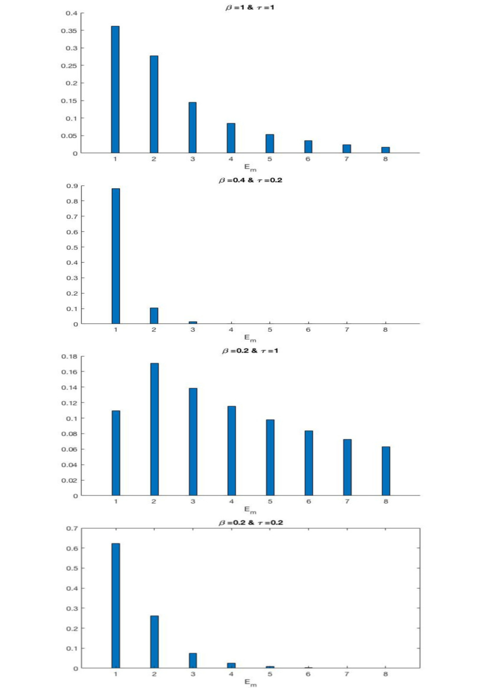
To give a concrete illustration, in Fig. 1 we have made a bar chart for the normalized number density $n_{0n\pm}/n_{0}$ in the different energy states for a few values of the temperature and magnetic field, under the assumption that the density is low enough for the system to be non-degenerate, i.e. assuming $T\gg T_{F}$.

As will be demonstrated in the next section, to a large degree the electrons behave as a multi-species system, where each particle species has its own rest mass, as given by Eq. 32 but with $p_{z}=0$. This is because the separation between Landau levels is on the order of the rest mass, and all excitation quanta with energies of that order have been neglected. If we define the effective number density of each ”species” (discrete energy-state) as

we see that $n_{0n\pm}$ essentially will be determined by the Boltzmann factors of Eq. 33. However, for the cases where our model Eq. 24 is of most interest, the magnetic field $B_{0}$ is strong enough to make relativistic Landau quantization prominent. Thus, in the next section and for the remainder of this paper, we will consider background distributions $W_{0\pm}$ where simplifications based on $\hbar\omega_{ce}/m\ll 1$ do not apply.

The operator in the square root in Eq. 24 gives the impression that it is very technical and complex to apply the model in studying, e.g., waves in plasma. In this section we consider electrostatic waves in a homogeneous plasma by using Eq. 24. We consider the wave vector $\mathbf{k}=k\mathbf{e}_{z}$ and express the momentum $\mathbf{p}$ in cylindrical coordinates $p_{\perp}$, $\varphi_{p}$, and $p_{z}$. To linearize Eq. 24, we separate variables according to $W_{\pm}=W_{0\pm}(p_{\perp},p_{z})+W_{1\pm}(z,p_{\perp},p_{z},t)$, $\mathbf{E}=E_{1}\mathbf{e}_{z}$ and $\mathbf{B}=B_{0}\mathbf{e}_{z}$, where the subscripts $0$ and $1$ denote unperturbed and perturbed quantities respectively. Moreover, the perturbed quantities follow the wave plane ansatz according to $W_{1\pm}=\tilde{W}_{1\pm}e^{ikz-i\omega t}$. Equation 24 is now

The unperturbed Wigner function $W_{0\pm}$ is given by the thermal background Wigner function in Eq. 33. Since the operators in $\epsilon^{\prime}_{\pm}$ have been shown to be energy eigenvalues when acting on $W_{0\pm}$; we act on both sides by $\left(\omega-kp_{z}/\epsilon^{\prime}_{\pm}\right)^{-1}$, such that the perturbed distribution function becomes

where in the second equality we used that $W_{0\pm}$ is a sum of eigenfunctions of $\epsilon^{\prime}_{\pm}$, and the summation is over the Landau levels indexed by $n$. Using Poisson’s equation, the dielectric tensor for the electrostatic case is

Note that if we set $\hbar$ to zero in $E_{n\pm}$ in the dielectric tensor, then the denominator in the the second term of the dielectric tensor is the same as for the relativistic Vlasov equation Alexandrov et al. 1984.

The background distribution $W_{0n\pm}$ will be divided into its eigenstates depending on the temperature and the magnetic field, see Fig. 1. As a result, the dispersion relation Eq. 42 is that of a relativistic multi-species plasma where each species has its own rest mass, $E_{n\pm}$.

In the present paper we have derived a kinetic model for plasmas immersed in a relativistically strong magnetic field, i.e., with a field strength of the order of the critical field. Based on a Foldy-Woythausen transformation and a Wigner transformation, an evolution equation for the spin-up and spin-down components $W_{\pm}$ has been found. Besides having two components, the main difference to a classical relativistic model is that the gamma-factor in that theory is replaced by an operator containing momentum derivatives. Since our theory is formulated in phase space, we stress that such operators are fundamentally different from the operators of Hilbert space, and to the best of our knowledge, this effect has not been seen in any previous quantum kinetic models. An immediate effect of the energy being an operator, comes when studying the background Wigner function. Classically, or in less advanced quantum mechanical models, the evolution equation does not predict the detailed momentum dependence for a given Landau level. Thus the background expression has been put in by hand, and one has to return to the starting point of the theory (e.g., the Pauli or Dirac equations for single particles) to find proper expressions. Here, however, the eigenvalue equation $\varepsilon^{\prime}W_{0}=E_{n,\pm}W_{0}$ determines the background state for a given Landau level (bar a constant for the number density), and there is no need to go outside the kinetic theory itself to find proper initial conditions.

To avoid some technical difficulties related to the operator orderings, we have here divided the magnetic field into an ultra-strong but constant part ($B_{0}\mathbf{\hat{z}}$) and a fluctuating part $\delta\mathbf{B}$. This approach allows for the treatment of large classes of problems in magnetar atmospheres, for example linear and nonlinear wave propagating in homogeneous backgrounds, even up to relativistic wave amplitudes, as long as the flutuating part fulfills $\mu_{B}\left|\delta\mathbf{B}\right|\ll m$.

Of course, a full modeling of the magnetar surroundings, covering the dipole nature of the background source field, is beyond the scope of such a theory. Moreover, in order to focus on the physics due to ultra-strong magnetic fields, the present theory excludes effects such as the magnetic dipole force, the spin magnetization, and the spin-orbit interaction included in some previous models Asenjo et al. 2012; Manfredi et al. 2019, which can be justified for the long scale lengths and moderate frequencies that we focus on here. In this context, however, it should be noted that omission of the spin-orbit interaction is closely related to a correction term of the free current density (see e.g. Eq. (21) of Ref. Asenjo et al. 2012). While the additional term kept by Ref. Asenjo et al. 2012 is a small correction for the conditions studied in this paper, it can contribute with currents perpendicular to $\mathbf{B}_{0}$ that may be of importance for certain problems, specifically for geometries where the (otherwise larger) parallel currents vanish. This and other possible extensions of the current theory is a project for future research.

To illustrate the usefulness of the present theory, we have computed the dispersion relation for Langmuir waves in a strong magnetic field for a relativistic temperature. To a large extent, we find that the electrons behave as if they are divided into different species. More concretely, each Landau level of the background plasma contributes to the susceptibility with a term similar to the classical relativistic expression, but with its own effective mass $m_{n\pm}=m\left(1+(2n+1\pm 1)\hbar\omega_{ce}/m\right)^{1/2}$. We expect this result to generalize to some other problems, but not be completely general, as for certain problems, the difference between the standard gamma factor and the energy expression of the current theory will be apparent. A more complete study of the effects due to ultra-strong magnetic fields is a project for future research.

References

- Haas (2011) F. Haas, Quantum plasmas: An hydrodynamic approach (Springer, New York, 2011).
- Shukla and Eliasson (2011) P. K. Shukla and B. Eliasson, Rev. Mod. Phys. 83, 885 (2011).
- Daligault (2014) J. Daligault, Phys. Plasmas 21, 040701 (2014).
- Materdey and Seyler (2003) T. B. Materdey and C. E. Seyler, Int. J. Mod. Phys. B 17, 4555 (2003).
- Yang and Yao (1991) B.-J. Yang and S.-G. Yao, Phys. Rev A 43, 1983 (1991).
- Misra et al. (2017) A. P. Misra, D. Chatterjee, and G. Brodin, Phys. Rev. E 96, 053209 (2017).
- Zamanian et al. (2010a) J. Zamanian, M. Marklund, and G. Brodin, New. J. Phys. 12, 043019 (2010a).
- Andreev (2017) P. A. Andreev, Phys. Plasmas 24, 022114 (2017).
- Andreev and Trukhanova (2018) P. A. Andreev and M. I. Trukhanova, J. Plasma Phys. 84 (2018).
- Asenjo et al. (2012) F. A. Asenjo, J. Zamanian, M. Marklund, G. Brodin, and P. Johansson, New. J. Phys. 14, 073042 (2012).
- Manfredi et al. (2019) G. Manfredi, P.-A. Hervieux, and J. Hurst, Rev. Mod. Plasma Phys. 3, 13 (2019).
- Ekman et al. (2017) R. Ekman, F. A. Asenjo, and J. Zamanian, Phys. Rev. E 96, 023207 (2017).
- Ekman et al. (2019) R. Ekman, H. Al-Naseri, J. Zamanian, and G. Brodin, Phys. Rev. E 100, 023201 (2019).
- Burton and Noble (2014) D. A. Burton and A. Noble, Contemp. Phys. 55, 110 (2014).
- (15) While the classical radiation reaction, where the response is a smooth function of the orbit, is a useful approximation as long as the emitted spectrum is soft (dominated by photons with energies well below ), the description based on QED (see e.g. Ilderton and Torgrimsson 2013; Cole et al. 2018), containing discrete probabilistic contributions due to the emission of high energy quanta, is more generally applicable.
- Eliezer et al. (2005) S. Eliezer, P. Norreys, J. T. Mendonça, and K. Lancaster, Phys. Plasmas 12, 052115 (2005).
- Harding and Lai (2006) A. K. Harding and D. Lai, Rep. Prog. Phys. 69, 2631 (2006).
- Uzdensky and Rightley (2014) D. A. Uzdensky and S. Rightley, Rep. Prog. Phys. 77, 036902 (2014).
- Stinebring et al. (1984) D. R. Stinebring, J. M. Cordes, J. M. Rankin, J. M. Weisberg, and V. Boriakoff, Astrophys. J. Supp. Ser. 55, 247 (1984).
- Rankin (1990) J. M. Rankin, Astrophys. J. 352, 247 (1990).
- Han et al. (1998) J. Han, R. Manchester, R. Xu, and G. Qiao, Mon. Not. R. Astron. Soc. 300, 373 (1998).
- Melrose and Weise (2009) D. B. Melrose and J. I. Weise, J. Phys. A 42, 345502 (2009).
- Asenjo et al. (2011) F. A. Asenjo, V. Muñoz, J. A. Valdivia, and S. M. Mahajan, Phys. Plasmas 18, 012107 (2011).
- Zamanian et al. (2010b) J. Zamanian, M. Stefan, M. Marklund, and G. Brodin, Physics of Plasmas 17, 102109 (2010b).
- Foldy and Wouthuysen (1950) L. L. Foldy and S. A. Wouthuysen, Phys. Rev. 78, 29 (1950).
- Silenko (2008) A. J. Silenko, Phys. Rev. A 77 (2008), 10.1103/physreva.77.012116.
- Silenko (2003) A. J. Silenko, Journal of Mathematical Physics 44, 2952 (2003), https://aip.scitation.org/doi/pdf/10.1063/1.1579991 .
- Transtrum and Van Huele (2005) M. K. Transtrum and J.-F. S. Van Huele, J. Math. Phys. 46, 063510 (2005).
- Stratonovich (1956) R. L. Stratonovich, Sov. Phys. D 1, 414 (1956), sov. Phys. Dokl. 1, 414 (1956).
- Kumar (1965) K. Kumar, Journal of Mathematical Physics 6, 1923 (1965), https://doi.org/10.1063/1.1704741 .
- Sheng et al. (2018) X.-L. Sheng, D. H. Rischke, D. Vasak, and Q. Wang, Eur. Phys. J. A 54, 21 (2018).
- Melrose and Parle (1983) D. B. Melrose and A. J. Parle, Aust. J. Phys. 36, 755 (1983).
- Alexandrov et al. (1984) A. F. Alexandrov, L. S. Bogdankevich, and A. A. Rukhadze, Principles of Plasma Electrodynamics (Springer-Verlag Berlin Heidelberg, 1984).
- Ilderton and Torgrimsson (2013) A. Ilderton and G. Torgrimsson, Phys. Lett. B 725, 481 (2013).
- Cole et al. (2018) J. M. Cole, K. T. Behm, E. Gerstmayr, T. G. Blackburn, J. C. Wood, C. D. Baird, M. J. Duff, C. Harvey, A. Ilderton, A. S. Joglekar, K. Krushelnick, S. Kuschel, M. Marklund, P. McKenna, C. D. Murphy, K. Poder, C. P. Ridgers, G. M. Samarin, G. Sarri, D. R. Symes, A. G. R. Thomas, J. Warwick, M. Zepf, Z. Najmudin, and S. P. D. Mangles, Phys. Rev. X 8, 011020 (2018).