跳到论文正文
W Papers独立论文阅读器 arXiv:2005.13686 论文正文 计算阅读时间 · 0%
引用这篇论文根据当前论文元数据生成,正式投稿前建议核对。


License: arXiv.org perpetual non-exclusive license
arXiv:2005.13686v1 [math.CO] 27 May 2020

Sorting probability of Catalan posets

Swee Hong Chan Swee Hong ChanDepartment of Mathematics, UCLA, Los Angeles, CA 90095. Email address: sweehong@math.ucla.edu , Igor Pak Igor PakDepartment of Mathematics, UCLA, Los Angeles, CA 90095. Email address: pak@math.ucla.edu and Greta Panova Greta PanovaDepartment of Mathematics, USC, Los Angeles, CA 90089. Email address: gpanova@usc.edu
Date: August 11, 2026
Abstract.

We show that the sorting probability of the Catalan poset PnP_{n} satisfies δ(Pn)=O(n−5/4)\delta(P_{n})=O\bigl(n^{-5/4}\bigr).

Key words and phrases: 
1/3–2/3 conjecture, Catalan numbers, Catalan posets, linear extension, sorting probability
2010 Mathematics Subject Classification
05A16, 06A07, 60C05

1. Introduction

The sorting probability of a poset PP, see below, is an interesting measure of independence of linear extensions of PP. Originally introduced in connection with sorting under partial information by Kislitsyn (1968) and Fredman (1975), it came to prominence as the subject of the celebrated 13\frac{1}{3}\hskip 1.70709pt–23\,\hskip 1.70709pt\frac{2}{3} Conjecture, see [Tro]. The conjecture received further acclaim in 1980s after a remarkable breakthrough by Kahn and Saks [KS], but remains open in full generality. We refer to [CPP, §\lx@sectionsign1.3] for a recent overview of the literature and further references.

In this paper we study the sorting probability δ⁡(Pn)\delta(P_{n}) of a Catalan poset PnP_{n} on 2​n2n elements, which is defined as a product of a chain with 2 elements and with nn elements: Pn:=C2×CnP_{n}:=C_{2}\times C_{n}. The name comes from the fact that the number of linear extensions of PnP_{n} is the Catalan number:

e⁡(Pn)=Cat​(n):=1n+1​(2​nn).e(P_{n})\,=\,{\text{\rm Cat}}(n)\,:=\,\frac{1}{n+1}\binom{2n}{n}.

With over numerous combinatorial interpretations and countless literature, Catalan numbers are extremely well studied, see e.g. [S1, S2]. It is thus remarkable that δ⁡(Pn)\delta(P_{n}) has been out of reach until now.

Formally, for a finite poset P=(X,≺)P=(X,\prec), let ℒP\mathcal{L}_{P} denote the set of linear extensions of PP, and let e⁡(P):=|ℒP|e(P):=|\mathcal{L}_{P}|. The sorting probability δ⁡(P)\delta(P) is defined as

δ(P):=minx,y∈X|P[L(x)≤L(y)]−P[L(y)≤L(x)]|,\delta(P)\hskip 1.70709pt:=\hskip 1.70709pt\min_{x,y\in X}\,\bigl|\hskip 0.85355pt{\text{\bf P}}\hskip 0.85355pt[L(x)\leq L(y)]\hskip 0.85355pt-\hskip 0.85355pt{\text{\bf P}}\hskip 0.85355pt[L(y)\leq L(x)\hskip 0.85355pt]\hskip 0.85355pt\bigr|\hskip 1.70709pt,

where L∈ℒPL\in\mathcal{L}_{P} is a uniform linear extension of PP. The 13\frac{1}{3}\hskip 1.70709pt–23\,\hskip 1.70709pt\frac{2}{3} Conjecture mentioned above, claims that δ⁡(P)≤13\delta(P)\leq\frac{1}{3} for all finite posets PP.

Theorem 1.

For the Catalan poset PnP_{n}, we have δ(Pn)=O(n−5/4)\delta(P_{n})=O\bigl(n^{-5/4}\bigr).

Until recently, there were very few results in this direction. First, it was shown by Linial, that δ⁡(Pn)≤13\delta(P_{n})\leq\frac{1}{3}, and in fact this holds for all posets of width two [Lin]. For indecomposable posets PP of width two, this general bound was slightly improved by Sah to δ⁡(P)<0.3225\delta(P)<0.3225 [Sah]. In an online discussion about for Catalan posets, the second author improved this bound to δ⁡(Pn)<0.2995\delta(P_{n})<0.2995, by comparing x=(1,17)x=(1,17), y=(2,3)y=(2,3) and taking nn large enough [P2]. In a different direction, Olson and Sagan showed in [OS], that δ⁡(Pλ)≤13\delta(P_{\lambda})\leq\frac{1}{3}, for all Young diagrams λ⊢n\lambda\vdash n, s.t. λ≠(n)\lambda\neq(n), (1n)(1^{n}).

In our recent paper [CPP], we showed that δ(Pn)=O(n−1/2)\delta(P_{n})=O\bigl(n^{-1/2}\bigr), giving the first bound that δ⁡(Pn)→0\delta(P_{n})\to 0 as n→∞n\to\infty. Thus Theorem 1 is a substantial improvement over this result. More generally, we showed that δ(Pλ)=O(n−1/2)\delta(P_{\lambda})=O\bigl(n^{-1/2}\bigr), for all partitions λ⊢n\lambda\vdash n with bounded length ℓ=ℓ⁡(λ)\ell=\ell(\lambda), and such that λℓ=Ω⁡(n)\lambda_{\ell}=\Omega(n). The tools in [CPP] rely on technical results in Algebraic Combinatorics. Here we present a more direct computation giving better bounds.

Figure 1. Catalan poset P4P_{4}, linear extension L∈ℒP4L\in\mathcal{L}_{P_{4}}, Young diagram λ=(4,4)\lambda=(4,4), the corresponding standard Young tableau A∈SYT⁡(λ)A\in\operatorname{{\rm SYT}}(\lambda), and Dyck path γ:(0,0)→(8,0)\gamma:(0,0)\to(8,0).

We have several motivations for studying the Catalan posets. On the one hand, they are a natural special case of general Young diagram posets PλP_{\lambda}, and Theorem 1 is perhaps an indication how sharp the general bounds in [CPP] are. On the other hand, they are closely related to the behavior of Brownian excursion, via the standard bijection from standard Young tableaux AA of shape (n,n)(n,n) to Dyck paths γ:(0,0)→(2​n,0)\gamma:(0,0)\to(2n,0), see Figure 1.

Curiously, the sorting probability has a natural probabilistic interpretation in terms of Dyck paths:

P[L(1,a)<L(2,b)]=P[γ passes above (a+b−1,a−b)].{\text{\bf P}}\hskip 0.85355pt\bigl[\hskip 0.85355ptL(1,a)<L(2,b)\hskip 0.85355pt\bigr]\,=\,{\text{\bf P}}\hskip 0.85355pt\bigl[\hskip 0.85355pt\text{$\gamma$ passes above $(a+b-1,a-b)$}\hskip 0.85355pt\bigr]\hskip 0.85355pt.

For example, for A∈SYT⁡(4,4)A\in\operatorname{{\rm SYT}}(4,4) as in the figure, let a=5a=5 and b=2b=2. Then we have A⁡(1,5)<A⁡(2,2)A(1,5)<A(2,2), and the corresponding path γ\gamma is above point p=(5,2)p=(5,2). Unfortunately the standard probabilistic tools for the Brownian excursion are too weak to establish Theorem 1, but they do give the right heuristic idea of how to approach the problem (see §\lx@sectionsign5.1). Thus we resort to a direct asymptotic analysis of the sorting probabilities.

Notation.

We write C1​(ε),C2​(ε),…C_{1}(\varepsilon),C_{2}(\varepsilon),\ldots to denote (effectively computable) positive constants that depend on a fixed parameter ε>0\varepsilon>0, but not on nn. Similarly, we write C1,C2,…C_{1},C_{2},\ldots to denote (effectively computable) absolute constants that do not depend on ε\varepsilon. In the paper, we identify PnP_{n} with Young diagram (n,n)(n,n), and linear extensions ℒPn\mathcal{L}_{P_{n}} with standard Young tableaux SYT⁡(n,n)\operatorname{{\rm SYT}}(n,n), see Figure 1. Here we use the matrix coordinates, so e.g. L⁡(2,3)=7L(2,3)=7, for LL as in the figure.

2. Sorting probability via lattice paths

Throughout the paper, let  I=[n10,9​n10]I=\bigl[\frac{n}{10},\hskip 0.85355pt\frac{9n}{10}\bigr]  and  J=[n10,10​n]J=\bigl[\frac{\sqrt{n}}{10},\hskip 0.85355pt10\hskip 0.85355pt\sqrt{n}\bigr]. Our approach to proving Theorem 1 is to carefully analyze the sorting probability function Rn​(h,z):I×J→[0,1]R_{n}(h,z):I\times J\to[0,1], defined as follows:

(2.1) Rn(h,z):=P[L(2,h−z)<L(1,h)],whereh∈I,z∈J.R_{n}(h,z)\,:=\,{\text{\bf P}}\hskip 0.85355pt\bigl[\hskip 1.70709ptL(2,h-z)\hskip 0.85355pt<\hskip 0.85355ptL(1,h)\hskip 0.85355pt\bigr],\ \ \text{where}\ \ h\in I,\ z\in J\hskip 0.85355pt.

Consider the lattice paths γ\gamma in ℕ2\mathbb{N}^{2} from (0,0)(0,0) to (n,n)(n,n), which move up and to the right and do not go below (Southeast) of the main diagonal (0,0)−−(n,n)(0,0)--(n,n). Denote by Cat​(n){\text{\it Cat}}(n) the set of such paths. Our intuition comes from the following combinatorial interpretation already mentioned in the introduction.

Proposition 2.

The sorting probability function Rn​(h,z)R_{n}(h,z) is equal to the probability of a lattice path γ∈Cat​(n)\gamma\in{\text{\it Cat}}(n) to pass Southeast (SE) of the point (h−z−12,h−12)(h-z-\frac{1}{2},h-\frac{1}{2}).

Proof.

This follows from the bijection between lattice paths γ∈Cat​(n)\gamma\in{\text{\it Cat}}(n) and linear extensions L∈ℒPnL\in\mathcal{L}_{P_{n}} via standard Young tableaux A∈SYT⁡(n,n)A\in\operatorname{{\rm SYT}}(n,n), as shown in Figure 1. Formally, let up-steps correspond to a square in the first row, and right-steps to squares in the second row. The details are straightforward. ∎

The next two lemmas describe the local behavior of the sorting probability function Rn​(h,z)R_{n}(h,z), in essence estimating discrete partial derivatives in both directions. These lemmas are key to the proof of Theorem 1. We prove the theorem in Section 3 and the lemmas in Section 4.

To simplify the notation, we extend this function to all real numbers: Rn​(h,z):=Rn​(⌊h⌋,⌊z⌋)R_{n}(h,z):=R_{n}\bigl(\lfloor h\rfloor,\lfloor z\rfloor\bigr).

Lemma 3.

For all  h∈Ih\in I  and  z∈Jz\in J, the sorting probability function satisfies:

(2.2) Rn​(h,n/10)≤14andRn​(h,10​n)≥34,R_{n}\left(h,\sqrt{n}/10\right)\,\leq\,\frac{1}{4}\,\quad\text{and}\quad R_{n}(h,10\sqrt{n})\,\geq\,\frac{3}{4}\hskip 1.70709pt,

and

(2.3) C1n≤Rn​(h,z+1)−Rn​(h,z)≤C2n,\frac{C_{1}}{\sqrt{n}}\,\leq\,R_{n}(h,z+1)-R_{n}(h,z)\,\leq\,\frac{C_{2}}{\sqrt{n}}\hskip 1.70709pt,

where C1,C2>0C_{1},\hskip 0.85355ptC_{2}>0 are universal constants, and nn is large enough.

In other words, the function Rn​(h,⋅)R_{n}(h,\cdot) is increasing and passing over 1/21/2 at some point in the interval JJ.

Lemma 4.

For all  h∈[n10,n+z+12]⊂Ih\in\bigl[\frac{n}{10},\frac{n+z+1}{2}\bigr]\subset I  and  z∈Jz\in J, the sorting probability function satisfies:

(2.4) Rn​(h,z)=Rn​(n+z−h,z),R_{n}(h,z)\hskip 1.70709pt=\hskip 1.70709ptR_{n}(n+z-h,z)\hskip 1.70709pt,

and

(2.5) C3​n−2​h+zn2≤Rn​(h,z)−Rn​(h+1,z)≤C4​n−2​h+zn2,C_{3}\hskip 1.70709pt\frac{n-2h+z}{n^{2}}\,\leq\,R_{n}(h,z)\hskip 1.70709pt-\hskip 1.70709ptR_{n}(h+1,z)\,\leq\,C_{4}\hskip 1.70709pt\frac{n-2h+z}{n^{2}}\hskip 1.70709pt,

where C3,C4>0C_{3},\hskip 0.85355ptC_{4}>0 are universal constants, and nn is large enough.

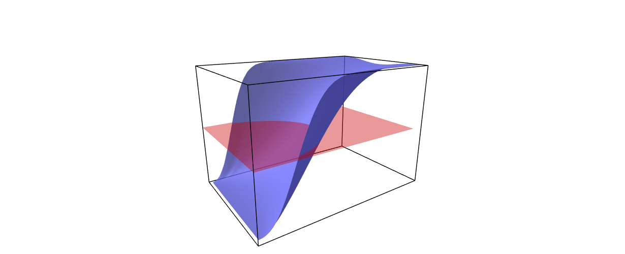
In other words, the function Rn​(⋅,z)R_{n}(\cdot,z) is symmetric, bimodal, and attains its minimum value at h=⌊n+z2⌋h=\lfloor\frac{n+z}{2}\rfloor. See Figure 2 and 5 for an illustration.
Refer to caption
Refer to caption
Figure 2. Left: Graph of the function S⁡(r,t)S(r,t) defined in §\lx@sectionsign5.1, which coincides with the limit surface of the sorting probability Rn​(h,z)R_{n}(h,z) when n→∞n\to\infty. We also draw the red plane at height  12\frac{1}{2}  to indicate positions of the best sorting pairs  x=(1,h)x=(1,h)  and  y=(1,h−z)y=(1,h-z). Right: The intersection between the plane and the surface on the left picture when n=1000n=1000. The plot is the function z=f⁡(h)z=f(h) that minimizes  |Rn​(h,z)−12|\bigl|R_{n}(h,z)-\frac{1}{2}\bigr|  for  h∈[0,n]h\in[0,n].

In fact, the symmetry follows from the central symmetry of the Catalan poset PnP_{n}:

P[L(2,b)<L(1,a)]=P[L(2,n−a)<L(1,n−b)],{\text{\bf P}}\hskip 0.85355pt\bigl[\hskip 1.70709ptL(2,b)\hskip 0.85355pt<\hskip 0.85355ptL(1,a)\hskip 0.85355pt\bigr]\,=\,{\text{\bf P}}\hskip 0.85355pt\bigl[\hskip 1.70709ptL(2,n-a)\hskip 0.85355pt<\hskip 0.85355ptL(1,n-b)\hskip 0.85355pt\bigr],

which proves (2.4).

3. Proof of Theorem 1

By Lemma 3, there exists z∈Jz\in J, so that

(3.1) 12−C2n≤Rn​(n/2,z)≤12.\frac{1}{2}\hskip 1.70709pt-\hskip 1.70709pt\frac{C_{2}}{\sqrt{n}}\ \leq\ R_{n}\bigl(n/2,z\bigr)\ \leq\ \frac{1}{2}\hskip 1.70709pt.

Let h0:=n/2−K​n3/4h_{0}:=n/2-K\hskip 0.85355ptn^{3/4}, where the constant K>0K>0 will be determined later. We have:

Rn​(h0,z)\displaystyle R_{n}(h_{0},z)\ =Rn​(n/2,z)+∑k=0⌊K​n3/4⌋Rn​(h0+k,z)−Rn​(h0+k+1,z)\displaystyle=\ R_{n}\bigl(n/2,z\bigr)\hskip 1.70709pt+\hskip 1.70709pt\sum_{k=0}^{\lfloor K\hskip 0.85355ptn^{3/4}\rfloor}\hskip 1.70709ptR_{n}(h_{0}+k,z)\hskip 1.70709pt-\hskip 1.70709ptR_{n}(h_{0}+k+1,z)
≥(2.5)Rn(n/2,z)+C3∑k=0⌊K​n3/4⌋|k−z|n2\displaystyle\geq_{\eqref{eq:R h-derivative}}\ R_{n}\bigl(n/2,z\bigr)\,+\,C_{3}\sum_{k=0}^{\lfloor K\hskip 0.85355ptn^{3/4}\rfloor}\hskip 1.70709pt\frac{|k-z|}{n^{2}}
≥Rn​(n/2,z)+C3​(K​n3/4)24​n2\displaystyle\geq\quad\ R_{n}\bigl(n/2,z\bigr)\,+\,C_{3}\frac{\bigl(K\hskip 1.70709ptn^{3/4}\bigr)^{2}}{4\hskip 1.70709ptn^{2}}
≥(3.1)12−C2n+C3​K24​n.\displaystyle\geq_{\eqref{eq:not tight}}\ \frac{1}{2}\,-\,\frac{C_{2}}{\sqrt{n}}\,+\,\frac{C_{3}\hskip 0.85355ptK^{2}}{4\sqrt{n}}\hskip 1.70709pt.

Taking K:=2​C2C3K:=2\sqrt{\frac{C_{2}}{C_{3}}}, we get

(3.2) Rn​(h0,z)≥12.R_{n}(h_{0},z)\ \geq\ \frac{1}{2}.

It then follows from (3.1) and (3.2), that

Rn​(n/2,z)≤12≤Rn​(h0,z).R_{n}\bigl(n/2,z\bigr)\,\leq\,\frac{1}{2}\,\leq\,R_{n}\bigl(h_{0},z\bigr).

Hence, there exists an integer h1∈[h0,n/2]h_{1}\in\left[h_{0},n/2\right], such that Rn​(h1+1,z)≤12≤Rn​(h1,z)R_{n}(h_{1}+1,z)\leq\frac{1}{2}\leq R_{n}(h_{1},z). We conclude:

12−Rn(h1+1,z)≤Rn(h1,z)−Rn(h1+1,z)≤(2.5)C42​K​n3/4+10​nn2=O(n−5/4).\displaystyle\frac{1}{2}\,-\,R_{n}(h_{1}+1,z)\ \leq\ R_{n}(h_{1},z)\hskip 1.70709pt-\hskip 1.70709ptR_{n}(h_{1}+1,z)\ \leq_{\eqref{eq:R h-derivative}}\ C_{4}\hskip 1.70709pt\frac{2Kn^{3/4}\hskip 0.85355pt+\hskip 0.85355pt10\sqrt{n}}{n^{2}}\ =\ O\bigl(n^{-5/4}\bigr).

This completes the proof of the theorem. □\square

Example 5.

The construction in the proof is quite delicate, as it is fundamentally discrete rather than continuous. In Figure 3, we show the graph of Rn​(h,z)R_{n}(h,z) with n=1000n=1000 and two values: z=33z=33 and z=34z=34. In the former case, the function intersects 12\hskip 0.85355pt\frac{1}{2}, and h1=439h_{1}=439 as in the proof. In the latter case, the function is always above 12\hskip 0.85355pt\frac{1}{2}.

Refer to caption
Refer to caption
Figure 3. Functions  R1000​(h,33)R_{1000}(h,33)  and  R1000​(h,34)R_{1000}(h,34).

4. Proof of lemmas

4.1. Preliminaries

For 0≤a≤b0\leq a\leq b, denote by f⁡(a,b)f(a,b) the number of paths γ:(0,0)→(a,b)\gamma:(0,0)\to(a,b) above diagonal y=xy=x.

Lemma 6 (The ballot theorem, see e.g. [Fel, §\lx@sectionsignIII.1]).

For 0≤a≤b0\leq a\leq b,

f⁡(a,b)=(a+ba)−(a+ba−1)=(a+ba)​b−a+1b+1.f(a,b)\ =\ \binom{a+b}{a}-\binom{a+b}{a-1}\ =\ \binom{a+b}{a}\frac{b-a+1}{b+1}.

Let pn​(a,b)p_{n}(a,b) be the probability that the lattice path γ∈Cat​(n)\gamma\in{\text{\it Cat}}(n) passes through the point (a,b)(a,b). By definition,

pn​(a,b)=f⁡(a,b)⋅f⁡(n−b,n−a)Cat​(n).p_{n}(a,b)\,=\,\frac{f(a,b)\cdot f(n-b,n-a)}{{\text{\rm Cat}}(n)}\hskip 1.70709pt.
Lemma 7 ([MP2, Thm 3.3]).

Fix ε,K>0\varepsilon,K>0. We have:

(4.1) pn(h−z,h)≤C1​(ε)⋅(z+1)2n3/2e−z2/n,p_{n}(h-z,h)\,\leq\,\frac{C_{1}(\varepsilon)\cdot(z+1)^{2}}{n^{3/2}}\,e^{-z^{2}/n}\hskip 0.85355pt,

for  ε​n≤h≤(1−ε)​n\varepsilon\hskip 0.85355ptn\hskip 0.85355pt\leq\hskip 0.85355pth\hskip 0.85355pt\leq\hskip 0.85355pt(1-\varepsilon)\hskip 0.85355ptn, and 0≤z<h0\leq z<h, and C1​(ε)C_{1}(\varepsilon) a constant independent of nn. Furthermore,

(4.2) C2​(ε,K)​(z+1)2n3/2≤pn​(h−z,h)≤C3​(ε,K)​(z+1)2n3/2for1≤z≤K​n,C_{2}(\varepsilon,K)\hskip 1.70709pt\frac{(z+1)^{2}}{n^{3/2}}\,\leq\,p_{n}(h-z,h)\,\leq\,C_{3}(\varepsilon,K)\hskip 1.70709pt\frac{(z+1)^{2}}{n^{3/2}}\quad\text{for}\quad 1\hskip 1.70709pt\leq z\hskip 1.70709pt\leq\hskip 1.70709ptK\hskip 0.85355pt\sqrt{n}\hskip 1.70709pt,

where h,zh,\hskip 0.85355ptz as above, and C2​(ε,K)C_{2}(\varepsilon,K), C3​(ε,K)>0C_{3}(\varepsilon,K)>0 are constants independent of nn.

In fact, when n→∞n\to\infty, the constants in the theorem are computed explicitly in [MP2], but only the upper and lower bounds are needed in the proof of Lemmas 3 and 4.

Let qn​(a,b)q_{n}(a,b) denote the probability that the lattice path γ∈Cat​(n)\gamma\in{\text{\it Cat}}(n) passes through both (a,b−1)(a,b-1) and (a,b)(a,b). Similarly, let rn​(a,b)r_{n}(a,b) denote the probability that the lattice path γ∈Cat​(n)\gamma\in{\text{\it Cat}}(n) passes through points (a,b−1)(a,b-1), (a,b)(a,b) and (a,b+1)(a,b+1). From Lemma 7, we immediately have:

(4.3) rn(h−z,h)≤qn(h−z,h)≤pn(h−z,h)≤C1​(ε)⋅(z+1)2n3/2e−z2/nr_{n}(h-z,h)\hskip 1.70709pt\leq\hskip 1.70709ptq_{n}(h-z,h)\hskip 1.70709pt\leq\hskip 1.70709ptp_{n}(h-z,h)\hskip 1.70709pt\leq\hskip 1.70709pt\frac{C_{1}(\varepsilon)\cdot(z+1)^{2}}{n^{3/2}}\,e^{-z^{2}/n}\hskip 0.85355pt\hskip 1.70709pt

This immediately gives the upper bound in

(4.4) C4​(ε,K)​(z+1)2n3/2≤rn​(h−z,h)≤qn​(h−z,h)≤C3​(ε,K)​(z+1)2n3/2for​ 1≤z≤K​n,C_{4}(\varepsilon,K)\hskip 1.70709pt\frac{(z+1)^{2}}{n^{3/2}}\hskip 1.70709pt\leq\hskip 1.70709ptr_{n}(h-z,h)\hskip 1.70709pt\leq\hskip 1.70709ptq_{n}(h-z,h)\hskip 1.70709pt\leq\hskip 1.70709ptC_{3}(\varepsilon,K)\hskip 1.70709pt\frac{(z+1)^{2}}{n^{3/2}}\quad\text{for}\ \ 1\hskip 1.70709pt\leq z\hskip 1.70709pt\leq\hskip 1.70709ptK\hskip 0.85355pt\sqrt{n}\hskip 1.70709pt,

The lower bound in (4.4) follows from

rn​(a,b)=f⁡(a,b−1)⋅f⁡(n−b−1,n−a)Cat​(n)=pn​(a,b)​(n−b)​(b−a)​(b−a+2)​(b+1)(2​n−a−b)​(b−a+1)2​(a+b).r_{n}(a,b)=\frac{f(a,b-1)\cdot f(n-b-1,n-a)}{{\text{\rm Cat}}(n)}\,=\,p_{n}(a,b)\hskip 1.70709pt\frac{(n-b)(b-a)(b-a+2)(b+1)}{(2n-a-b)(b-a+1)^{2}(a+b)}\hskip 1.70709pt.

Indeed, for b=hb=h and a=h−z=b−o⁡(b)a=h-z=b-o(b), one can take C4​(ε,K)=C2​(ε,K)/5C_{4}(\varepsilon,K)=C_{2}(\varepsilon,K)/5 for h>ε​nh>\varepsilon n large enough.

4.2. Proof of Lemma 3

By Proposition 2, the sorting probability function Rn​(h,z)R_{n}(h,z) is the probability that the vertical step at height hh of a random lattice path γ∈Cat​(n)\gamma\in{\text{\it Cat}}(n) happens at x≥h−zx\geq h-z. This gives:

(4.5) Rn​(h,z)=∑k=1zqn​(h−k,h).R_{n}(h,z)\,=\,\sum_{k=1}^{z}\hskip 1.70709ptq_{n}(h-k,h)\hskip 0.85355pt.

Since qn​(h−k,h)≥0q_{n}(h-k,h)\geq 0, it then follows that Rn​(h,⋅)R_{n}(h,\cdot) is an increasing function for every hh.

Now set ε=110\varepsilon=\frac{1}{10}, K=10K=10, and let ε​n≤h≤(1−ε)​n\varepsilon\hskip 0.85355ptn\leq h\leq(1-\varepsilon)\hskip 0.85355ptn. We have:

Rn​(h,n/10)\displaystyle R_{n}\bigl(h,\sqrt{n}/10\bigr)\ =∑k=1n/10qn​(h−k,h)≤∑k=1n/10(4.4)⁡C3​(ε,K)​(k+1)2n3/2\displaystyle=\ \sum_{k=1}^{\sqrt{n}/10}\hskip 1.70709ptq_{n}(h-k,h)\ \leq_{\eqref{eq:visit edge 2}}\ \sum_{k=1}^{\sqrt{n}/10}\hskip 1.70709ptC_{3}(\varepsilon,K)\frac{(k+1)^{2}}{n^{3/2}}
≤C3​(ε,K)​(n/10)3n3/2=C3​(ε,K)1000.\displaystyle\leq\,C_{3}(\varepsilon,K)\hskip 1.70709pt\frac{\bigl(\sqrt{n}/10\bigr)^{3}}{n^{3/2}}\ =\ \frac{C_{3}(\varepsilon,K)}{1000}\hskip 1.70709pt.

A direct computer calculation shows that

C3​(110,10)1000<14.\frac{C_{3}\bigl(\frac{1}{10},10\bigr)}{1000}\hskip 1.70709pt<\hskip 1.70709pt\frac{1}{4}\hskip 1.70709pt.

This proves the first inequality in (2.2).

On the other hand, we have:

Rn​(h,K​n)\displaystyle R_{n}\left(h,{K\sqrt{n}}\right)\, =∑k=1K​nqn​(h−k,h)= 1−∑k>K​nqn​(h−k,h)\displaystyle=\ \sum_{k=1}^{{K\sqrt{n}}}\hskip 1.70709ptq_{n}(h-k,h)\ =\ 1\hskip 1.70709pt-\hskip 1.70709pt\sum_{k>{K\sqrt{n}}}q_{n}(h-k,h)
≥(4.3) 1−C1(ε)∑k>K​n(z+1)2n3/2e−z2/n\displaystyle\geq_{\eqref{eq:visit edge 1}}\ 1\hskip 1.70709pt-\hskip 1.70709ptC_{1}(\varepsilon)\hskip 1.70709pt\sum_{k>{K\sqrt{n}}}\hskip 1.70709pt\frac{(z+1)^{2}}{n^{3/2}}\hskip 1.70709pte^{-z^{2}/n}
≳ 1−C1​(ε)​∫K∞x2​e−x2​𝑑x.\displaystyle\gtrsim\quad\ 1\hskip 1.70709pt-\hskip 1.70709ptC_{1}(\varepsilon)\hskip 1.70709pt\int_{K}^{\infty}\hskip 1.70709ptx^{2}\hskip 0.85355pte^{-x^{2}}\hskip 1.70709ptdx\hskip 0.85355pt.

A direct computer calculation shows that for ε=110\varepsilon=\frac{1}{10} and K=10K=10, we have:

C1​(0.1)​∫10∞x2​e−x2​𝑑x<14.C_{1}\bigl(0.1\bigr)\,\int_{10}^{\infty}\hskip 1.70709ptx^{2}\hskip 0.85355pte^{-x^{2}}\,dx\,<\,\frac{1}{4}\hskip 1.70709pt.

This proves the second inequality in (2.2).

For (2.3), let h∈Ih\in I, z∈Jz\in J be as in the lemma. We have:

Rn(h,z+1)−Rn(h,z)=(4.5)qn(h−(z+1),h)\displaystyle R_{n}(h,z+1)\hskip 1.70709pt-\hskip 1.70709ptR_{n}(h,z)\ =_{\eqref{eq:sum q}}\ q_{n}(h-(z+1),h)

and the bounds now follow from (4.2). This completes the proof of the Lemma 3. □\square

4.3. Bimodality

The following lemma is used in the proof of Lemma 4 in the next section.

Lemma 8.

Let h∈[1,n−1]h\in[1,n-1]and z∈[1,h−1]z\in[1,h-1]. Then Rn​(h,z)>Rn​(h+1,z)R_{n}(h,z)>R_{n}(h+1,z) if and only if h≤12​(n+z)h\leq\frac{1}{2}(n+z)\hskip 0.85355pt.

Proof.

Let A=(h−z+1/2,h+1/2)A=(h-z+1/2,h+1/2) and B=(h−z−1/2,h−1/2)B=(h-z-1/2,h-1/2) be two points in the plane. By Proposition 2, the sorting probabilities Rn​(h+1,z)R_{n}(h+1,z) and Rn​(h,z)R_{n}(h,z) are probabilities that the lattice path γ∈Cat​(n)\gamma\in{\text{\it Cat}}(n) passes to SE of the points AA and BB, respectively. Denote by N1N_{1} and N2N_{2}, respectively, the numbers of these paths. Then we have:

Rn​(h,z)−Rn​(h+1,z)=1Cat​(n)​(N2−N1).R_{n}(h,z)\hskip 1.70709pt-\hskip 1.70709ptR_{n}(h+1,z)\,=\,\frac{1}{{\text{\rm Cat}}(n)}\hskip 1.70709pt\bigl(N_{2}\hskip 1.70709pt-\hskip 1.70709ptN_{1}\bigr).

Let x:=h+1−zx:=h+1-z. Denote by M1M_{1} and M2M_{2} the number of paths γ∈Cat​(n)\gamma\in{\text{\it Cat}}(n) which contain segments (x−2,h)→(x,h)(x-2,h)\to(x,h) and (x−1,h−1)→(x−1,h+1)(x-1,h-1)\to(x-1,h+1) , respectively. Note that N2−N1N_{2}-N_{1} is exactly the difference between the numbers of paths passing below point AA but above BB, and the paths passing left of AA but right of BB. Thus, N2−N1=M2−M1N_{2}-N_{1}=M_{2}-M_{1}.

Figure 4. The two types of paths in the proof of Lemma 8, with M1M_{1} counting blue paths and M2M_{2} red paths.

We have:

M1\displaystyle M_{1} =f⁡(x−2,h)​f​(n−h,n−x)=(x+h−2x−2)​(2​n−x−hn−h)​(h−x+3)​(h−x+1)(h+1)​(n−x+1),\displaystyle=\,f(x-2,h)\hskip 1.70709ptf(n-h,n-x)\,=\,\binom{x+h-2}{x-2}\binom{2n-x-h}{n-h}\frac{(h-x+3)(h-x+1)}{(h+1)(n-x+1)}\hskip 1.70709pt,
M2\displaystyle M_{2} =f⁡(x−1,h−1)​f​(n−h−1,n−x+1)=(x+h−2x−1)​(2​n−x−hn−h−1)​(h−x+3)​(h−x+1)h⁡(n−x+2)\displaystyle=\,f(x-1,h-1)\hskip 1.70709ptf(n-h-1,n-x+1)\,=\,\binom{x+h-2}{x-1}\binom{2n-x-h}{n-h-1}\frac{(h-x+3)(h-x+1)}{h(n-x+2)}

and therefore:

M2−M1=(x+h−2x−1)​(2​n−x−hn−h−1)​(h−x+1)​(h−x+2)​(h−x+3)​(n−x−h+1)h⁡(h+1)​(n−h)​(n−x+2).\displaystyle M_{2}\hskip 1.70709pt-\hskip 1.70709ptM_{1}\,=\,\binom{x+h-2}{x-1}\binom{2n-x-h}{n-h-1}\frac{(h-x+1)(h-x+2)(h-x+3)(n-x-h+1)}{h(h+1)(n-h)(n-x+2)}.

The last expression is ≥0\geq 0 if and only if h+x≤n+1h+x\leq n+1, and the result follows. ∎

4.4. Proof of Lemma 4

Equation (2.4) is proved earlier. For (2.5), from the proof of Lemma 8 we have:

Rn​(h,z)−Rn​(h+1,z)=M2Cat​(n)​(z+1)​(n−2​h+z)(h+1)​(n−h)=rn​(h−z,z)​(z+1)​(n−2​h+z)(h+1)​(n−h).R_{n}(h,z)\hskip 1.70709pt-\hskip 1.70709ptR_{n}(h+1,z)\,=\,\frac{M_{2}}{{\text{\rm Cat}}(n)}\hskip 1.70709pt\frac{(z+1)(n-2h+z)}{(h+1)(n-h)}\,=\,r_{n}(h-z,z)\hskip 1.70709pt\frac{(z+1)(n-2h+z)}{(h+1)(n-h)}\hskip 1.70709pt.

Since z∈Jz\in J, we have:

rn(h−z,z)=(4.2)Θ(1n).r_{n}(h-z,z)\,=_{\eqref{eq:visit vertex 2}}\,\Theta\left(\frac{1}{\sqrt{n}}\right).

On the other hand, since h∈Ih\in I and z∈Jz\in J, we have:

(z+1)​(n−2​h+z)(h+1)​(n−h)=Θ⁡(nn2​(n−2​h+z)).\frac{(z+1)(n-2h+z)}{(h+1)(n-h)}\,=\,\Theta\left(\frac{\sqrt{n}}{n^{2}}\hskip 1.70709pt\bigl(n-2h+z\bigr)\right).

Combining these two asymptotics, we conclude:

Rn​(h,z)−Rn​(h+1,z)=Θ⁡(n−2​h+zn2).R_{n}(h,z)\hskip 1.70709pt-\hskip 1.70709ptR_{n}(h+1,z)\,=\,\Theta\left(\frac{n-2h+z}{n^{2}}\right).

This proves (2.5) and completes the proof of Lemma 4. □\square

5. Final remarks and open problems

5.1.

The sorting probability function Rn​(h,z)R_{n}(h,z) is the discrete version of the continuous function

S(t,r):=P[B0+(t)≥r],S(t,r)\,:=\,{\text{\bf P}}\hskip 0.85355pt\bigl[B_{0}^{+}(t)\geq r\bigr]\hskip 0.85355pt,

where B0+B_{0}^{+} is the Brownian excursion on [0,1][0,1], defined as the standard Brownian motion conditioned on the event B0+​(0)=B0+​(1)=0B_{0}^{+}(0)=B_{0}^{+}(1)=0 and B0+​(t)>0B_{0}^{+}(t)>0, for all t∈(0,1)t\in(0,1). It has the following explicit density formula (see e.g., [IM, Pit]):

S⁡(t,r)=22​π​t3​(1−t3)​∫0rx2​exp⁡(−x22​t​(1−t))​𝑑x,S(t,r)\ =\ \frac{2}{\sqrt{2\pi\hskip 0.85355ptt^{3}\hskip 0.85355pt(1-t^{3})}}\hskip 0.85355pt\int_{0}^{r}x^{2}\hskip 0.85355pt\exp\left(\frac{-x^{2}}{2t\hskip 0.85355pt(1-t)}\right)\,dx\hskip 0.85355pt,

see Figure 2. It is shown by Kaigh [Kai] that Rn​(h,z)R_{n}(h,z) converges to S⁡(hn,z2​n)S\left(\frac{h}{n},\frac{z}{\sqrt{2n}}\right) as n→∞n\to\infty. Unfortunately, the error terms of this convergence are too weak to imply Theorem 1. See Figure 5 for a plot comparing functions SS and R200R_{200} side by side, and note that these graphs appear nearly identical on this scale.

Refer to caption
Refer to caption
Figure 5. Left:  The plot of  Rn​(t​n,n/2)R_{n}(tn,\sqrt{n}/2), where  t∈(0,1)t\in(0,1)  and n=200n=200. Right:  The plot of the probability  1−S⁡(t,r)1-S(t,r), where  t∈(0,1)t\in(0,1)  and  r=2/4r=\sqrt{2}/4.

5.2.

Lemma 7 proved in [MP2] is one of many results in the context of the limit shape of pattern avoiding permutations, see e.g. [Kit] for an extensive overview of pattern avoidance. Many strongly related results are obtained in this direction, too many to list. Let us single out papers [AM, MP1] which are independent of [MP2], but cover the same pattern avoidance problem which translates into asymptotics of Dyck paths. Let us also mention two followup papers [HRS1, HRS2] which rederives and extends results in [MP1, MP2] via Brownian excursions.

5.3.

In answering the second author’s question [P2], Richard Stanley found the following curious limit formulas:

(5.1) limn→∞𝔼⁡[L⁡(1,k−1)]= 2​k−k​(2​kk)4k−1,limn→∞𝔼⁡[L⁡(2,k)]= 2​k+k​(2​kk)4k−1,\lim_{n\to\infty}\hskip 1.70709pt\mathbb{E}\bigl[L(1,k-1)\bigr]\,=\,2k\hskip 1.70709pt-\hskip 1.70709pt\frac{k\binom{2k}{k}}{4^{k-1}}\,,\quad\lim_{n\to\infty}\hskip 1.70709pt\mathbb{E}\bigl[L(2,k)\bigr]\,=\,2k\hskip 1.70709pt+\hskip 1.70709pt\frac{k\binom{2k}{k}}{4^{k-1}}\,,

where the expectation is over random L∈ℒ⁡(Pn)L\in\mathcal{L}(P_{n}). The limits for probabilities 𝐏[L(1,a)<(2,b)]\mathbf{P}\bigl[L(1,a)<(2,b)\bigr] for fixed a>b≥1a>b\geq 1 also exist, but much less elegant. Stanley asked whether there are elegant expectation formulas similar to (5.1), for other partitions λ=n​α\lambda=n\alpha.

In principle, using the technology in [KS, Saks], one can use (5.1) to show that δ⁡(Pn)<1e+ε\delta(P_{n})<\frac{1}{e}+\varepsilon for all ε>0\varepsilon>0 and nn large enough. Note that in [CPP] we already showed that δ⁡(Pλ)=O⁡(1/n)\delta(P_{\lambda})=O(1/\sqrt{n}) for the general TVK case λ=n​α\lambda=n\alpha.

5.4.

It would be interesting to see how tight Theorem 1 is. Let

(5.2) α:=lim infn→∞log⁡δ⁡(Pn)log⁡nandβ:=lim supn→∞log⁡δ⁡(Pn)log⁡n.\alpha\,:=\,\liminf_{n\to\infty}\hskip 1.70709pt\frac{\log\delta(P_{n})}{\log n}\quad\text{and}\quad\beta\,:=\,\limsup_{n\to\infty}\hskip 1.70709pt\frac{\log\delta(P_{n})}{\log n}\,.

We conjecture that

(5.3) −∞<α<β=−54.-\infty\,<\,\alpha\,<\,\beta\,=\,-\frac{5}{4}\,.

In other words, we believe that our upper bound is asymptotically tight. On the other hand, we believe that the lower bound is substantially smaller, but still polynomial. This has to do with the fact that lim inf\liminf depends on number theoretic properties of nn governing the position of 12\frac{1}{2} in the interval [R⁡(h+1,z),R⁡(h,z)]\bigl[R(h+1,z),\hskip 0.85355ptR(h,z)\bigr]. At the moment, we cannot even prove that δ⁡(Pn)>0\delta(P_{n})>0 for all n≥3n\geq 3. Finally, most speculatively, we conjecture that

(5.4) δ(Pn)=o(n−5/4).\delta(P_{n})\hskip 1.70709pt=\hskip 1.70709pto\bigl(n^{-5/4}\bigr)\hskip 0.85355pt.

We refer to [CPP, §\lx@sectionsign12-13] for further discussions and conjectures on the sorting probability.

5.5.

Our computer calculations show that the sorting probability δ⁡(Pn)\delta(P_{n}) has an erratic behavior, but seem to fit well Theorem 1 and the conjectures above. The first graph in Figure 6 shows that δ⁡(n)​n5/4\delta(n)\hskip 0.85355ptn^{5/4} is always less than 33, but frequently greater than 11, and greater than 13\frac{1}{3} at least half the time. While this may seem to point against (5.4), we believe it holds since a simple regression does indicate a very slow trend downwards.

Similarly, the second graph in Figure 6 shows that logn⁡δ⁡(n)\log_{n}\delta(n) is frequently smaller than −54-\frac{5}{4}, but is never too small, suggesting that −3<α<32-3<\alpha<\frac{3}{2} , in the notation of (5.2). Perhaps, going far beyond n=1000n=1000 would give further evidence in support or against the conjectures above. See the full sequences δ⁡(Pn)​Cat​(n)\delta(P_{n})\hskip 0.85355pt{\text{\rm Cat}}(n) and 12​(1−δ⁡(Pn))​Cat​(n)\frac{1}{2}(1-\delta(P_{n}))\hskip 0.85355pt{\text{\rm Cat}}(n) at [OEIS, A335212] and [OEIS, A335213], respectively.

Refer to caption
Refer to caption
Figure 6. Graphs of  δ⁡(Pn)​n5/4\delta(P_{n})\hskip 1.70709ptn^{5/4}  and  logn⁡δ⁡(Pn)\log_{n}\delta(P_{n}), for  3≤n≤10003\leq n\leq 1000.

5.6.

By the proof of Lemma 8, the integer N2−N1≥0N_{2}-N_{1}\geq 0 for h≤12​(n+z)h\leq\frac{1}{2}(n+z). This is a fundamentally combinatorial statement about the difference in the number of certain lattice paths, somewhat similar in nature to the super Catalan numbers, see e.g. [P1, §\lx@sectionsign4.5] for the references. It would be interesting to find an explicit combinatorial interpretation for (N2−N1)(N_{2}-N_{1}).

Acknowledgements

We are grateful to Sam Hopkins, Han Lyu and Richard Stanley for interesting discussions and useful comments, and to MathOverflow for providing a convenient platform for such discussions. The last two authors were partially supported by the NSF.

References

  • [AM] M. Atapour and N. Madras, Large deviations and ratio limit theorems for pattern-avoiding permutations, Combin. Probab. Comput. 23 (2014), 161–200.
  • [CPP] S. H. Chan, I. Pak and G. Panova, Sorting probability for large Young diagrams, arXiv:2005.08390, 38 pp.
  • [Fel] W. Feller, An introduction to probability theory and its applications, Vol. I (third ed.), John Wiley, New York, 1968, 509 pp.
  • [HRS1] C. Hoffman, D. Rizzolo and E. Slivken, Pattern-avoiding permutations and Brownian excursion Part I: shapes and fluctuations, Random Structures Algorithms 50 (2017), 394–419.
  • [HRS2] C. Hoffman, D. Rizzolo and E. Slivken, Pattern-avoiding permutations and Brownian excursion Part II: fixed points, Probab. Theory Related Fields 169 (2017), 377–424.
  • [IM] K. Itô and H. McKean, Diffusion processes and their sample paths, Springer, Berlin, 1974, 321 pp.
  • [KS] J. Kahn and M. Saks, Balancing poset extensions, Order 1 (1984), 113–126.
  • [Kai] W. D. Kaigh, An invariance principle for random walk conditioned by a late return to zero, Ann. Probab. 4 (1976), 115–121.
  • [Kit] S. Kitaev, Patterns in permutations and words, Springer, Heidelberg, 2011, 494 pp.
  • [Lin] N. Linial, The information-theoretic bound is good for merging, SIAM J. Comput. 13 (1984), 795–801.
  • [MP1] N. Madras and L. Pehlivan, Structure of random 312-avoiding permutations, Random Structures Algorithms 49 (2016), 599–631.
  • [MP2] S. Miner and I. Pak, The shape of random pattern-avoiding permutation, Adv. Appl. Math. 55 (2014), 86–130.
  • [OS] E. J. Olson and B. E. Sagan, On the 13\frac{1}{3}–23\frac{2}{3} conjecture, Order 35 (2018), 581–596.
  • [P1] I. Pak, Complexity problems in enumerative combinatorics, arXiv:1803.06636, 31 pp., an expanded version of the paper in Proc. ICM Rio de Janeiro, Vol. 3, 2018, 3139–3166.
  • [P2] I. Pak, Coincidences between average Catalan tableaux, MathOverflow, Question 331579 (May 15, 2019), https://tinyurl.com/ybhvh4hv.
  • [Pit] J. Pitman, Combinatorial stochastic processes, Springer, Berlin, 2006, 256 pp.
  • [Sah] A. Sah, Improving the 13\frac{1}{3}–23\frac{2}{3} conjecture for width two posets, 20 pp.; arXiv:1811.01500.
  • [Saks] M. Saks, Balancing linear extensions of ordered sets, Order 2 (1985), 327–330.
  • [OEIS] N. J. A. Sloane, The Online Encyclopedia of Integer Sequences, oeis.org.
  • [S1] R. P. Stanley, Enumerative Combinatorics, vol. 1 (second ed.) and vol. 2, Cambridge Univ. Press, 2012 and 1999.
  • [S2] R. P. Stanley, Catalan numbers, Cambridge Univ. Press, 2015, 215 pp.
  • [Tro] W. T. Trotter, Partially ordered sets, in Handbook of combinatorics, Vol. 1, Elsevier, Amsterdam, 1995, 433–480.