Performance analysis and optimization of power systems with spatially correlated noise

The electrical grid is witnessing major changes in its planning and operation, mainly driven by economic and environmental concerns [1]. A better understanding of today’s deployment of renewable resources in power systems will necessarily go through the analysis of the ramifications of the integration of power electronics on grid stability. During the gradual retirement of synchronous machines and its replacement by DC/AC converters in closed loop with efficient controllers, designed to emulate the electro-mechanical interaction inherently present in synchronous machines, mixed power generation seems to be inevitable, and the operation of DC/AC converters is conducted in a first step in the presence of synchronous machines [2].

In this context, Stochastic Differential Equations (SDEs) have gained more and more attention in the literature of power systems, motivated by its potential applications in modeling disturbances ubiquitous in real-life power grid [3]. A systematic and generic approach on how to model power systems as continuous-time SDEs subject to independent Wiener processes was developed in [3]. Gaussian processes have been adopted to model power fluctuations in [4]. In [5], the performance and stability analysis of low-inertia power grid were considered with both additive and multiplicative noises which model stochastic inertia behavior. Examples included also non-Gaussian disturbance for wind power uncertainty [6].

To assess the effect of disturbances on the system stability, different approaches have been adopted. We distinguish two main avenues, related to convergence properties of the SDE solution. First, strong convergence, i.e., with respect to a particular stochastic process trajectory, has been studied extensively in the literature that ranges from stability in probability, almost sure (exponential) synchronization [7], transient stability probability, such as the probability of frequency synchronization or voltage collapse [3]. Second, weak convergence, i.e., with respect to statistical properties of the solution, has also attracted interest in the analysis of power systems performance. A variety of recent considerations in the literature deals with weak convergence via quantitative understanding of the disturbance-to-output behavior. One possibility is $\mathcal{H}_{\infty}$ norm [8], primarily concerned with peaks in the frequency response following an event and the location of the worst case disturbance. Step response notions like, frequency nadir defined as the worst frequency drop, and the rate of change of frequency (RoCoF) as the maximal slope of frequency change during transients, are also common metrics in the study of the effect of disturbances on frequency stability.

While Linear Quadratic Regulator (LQR) formulations [9] remain sensitive to the choice of the time horizon apparent in the objective function [10], one attractive approach goes by $\mathcal{H}_{2}$ norm calculation [11, 12, 13]. $\mathcal{H}_{2}$ norm indicates root mean square or average sensitivity of the system performance to disturbances and is derived from a generalized Lyapunov equation [5]. For this, $\mathcal{H}_{2}$ norm approach has been leveraged, at many occasions in the form of an input-to-output measure, e.g. for the total resistive losses incurred in returning a power network of identical generators with resistive and inductive lines, to a synchronous state [12], common local and inter-area oscillations [11], and inertia and damping allocation, with specified capacity and budget constraints for DC/AC converters [13, 10].

Most of the analytical results consider homogeneous power system networks, where all the machines or generation units are identical and with uncorrelated white noise of unit variance. Only recently, heterogeneous inertia and damping are considered, within a stochastic setting in [14] under mild restrictions, which consist in machine dynamics proportional to nominal rating and fixed damping to inertia ratio of all the machines. In a second occasion, two differently parameterized behaviors (grid-forming and grid-following) of closed-loop DC/AC converters have been investigated and compared with simulative examples in [10], for optimal inertia and damping allocation, but not simultaneously. In [15], the stability of a mixed-generation comprising synchronous machines together with DC/AC converter based on model reduction, was considered but in a deterministic setup that does not include stochastic disturbances.

Compared to the existing literature, the contributions of this paper can be summarized as follows. We first derive an SDE model of heterogeneous power networks, extending previous models to more realistic setups, where parametric heterogeneity and spatial noise correlation with random initial conditions, enter the picture. For this, the generation units (which can be thought of as, either synchronous machines or closed-loop DC/AC converters, or both) have non-uniform inertia and damping. The normally distributed and spatially correlated noise models the practical setup, where a generation unit is affected by its neighbor’s noise and hence propagated according to graph Laplacian, e.g. cascaded failures, network outage, and voltage collapse [16]. Our second main result consists in the derivation of bounds on the $\mathcal{H}_{2}$ norm of the heterogeneous power system, based on a closed-form of the norm of the homogeneous power system model. We then demonstrate its utility by formulating and extending important optimization scenarios in design and control of power system networks.

In fact, in a mixed-generation framework, where the interplay between DC/AC converters in closed-loop with a machine emulating controller (e.g., droop [17] and matching control [18], virtual synchronous machines [19]) and synchronous machines is investigated, we pose possible scenarios for performance optimization, with respect to the derived $\mathcal{H}_{2}$ norm. We formulate an optimal susceptance problem to specify the optimal susceptances in a mixed generation (DC/AC converters and or synchronous machines). We additionally present an optimal node-edge assignment problem for an optimal pairing of generation units that improves the system performance in the $\mathcal{H}_{2}$ norm sense. Finally, we extend the inertia and damping allocation problem from [13] of DC/AC converters, subject to operational and budget constraints. We validate our analytical results for optimal damping and inertia, on adapted setup from Kundur’s four-machine two-area system [16].

The remainder of this paper unfurls as follows. Section II formulates and derives the heterogeneous SDE power systems model, starting from the classical swing equation. In Section III, we determine a closed form of system $\mathcal{H}_{2}$ norm, and interpret its dependence on network parameters. In Section IV, we formulate possible optimization scenarios with respect to system norm accounting for optimal susceptances and network topology, as well as an extension of inertia and damping allocation for proper deployment of DC/AC converters in the presence of synchronous machines. Finally, Section V validates our results by numerical simulations of an adapted Kundur’s 4-machine 2-area system.

We consider a heterogeneous power systems model, defined by a graph ${G}=(\mathcal{V},\mathcal{E})$ of an undirected network, where $\mathcal{V}$ is the set of $n$ heterogeneous generation units (i.e., buses), where inductive load with constant susceptance is considered and absorbed in the lines (e.g. after Kron reduction [20]). Let $\mathcal{E}$ be the set of $m$ edges (purely inductive lines) with weight susceptance $b_{e}>0,\,e\in\mathcal{E}$. We denote by $\mathcal{B}\in\real^{n\times m}$ the incidence matrix of the graph ${G}$, and by $\mathcal{N}_{i}$ the neighbor set of the $i$-th generation unit (DC/AC converter in closed-loop with droop control or synchronous machines). The voltage magnitude $V_{i}$ at the $i$-th bus is assumed to be constant and equal to one per unit. Under the approximation of quasi-stationary steady state, the swing equation of the $i$-th generation with inertial constant $m_{i}>0$, damping coefficient $d_{i}>0$, and (virtual) voltage phase angle $\theta_{i}\in\real$ describes the $i$-th node dynamics as follows,

where $P_{m,i}\in\real$ is constant mechanical power, and $P_{e,i}=\sum_{j\in\mathcal{N}_{i}}b_{ij}V_{i}V_{j}\sin(\theta_{i}-\theta_{j})=\sum_{j\in\mathcal{N}_{i}}b_{ij}\sin(\theta_{i}-\theta_{j})$ is the electrical power injected from $i$-th generation into the neighbor set $\mathcal{N}_{i}$ and vice versa. The disturbance $\eta_{i}(t),\,t>0$ stands for load fluctuations in renewable generation for DC/AC converters, or generator outages for synchronous machines.

The graph G is described by the weighted Laplacian matrix $L=\mathcal{B}\,\Gamma\,\mathcal{B}^{\top}\in\real^{n\times n}$, in function of $\Gamma=\text{diag}(b_{e})_{e\in\mathcal{E}}\in\real^{m\times m}$, with eigenvalues of a non-decreasing order $\lambda_{1}(L)=0<\lambda_{2}(L)\leq\dots\leq\lambda_{n}(L)$. Let $\mathrm{d}w_{i}(t)$ be the increment of the $i$- th standard Wiener process $w_{i}(t)$ that results in the disturbance $\eta_{i}(t)=\frac{\mathrm{d}w_{i}(t)}{\mathrm{d}t}$. The disturbance $\eta_{i}(t)$, resulting from the process $w_{i}(t)$ at node $i$ is correlated to the disturbance $\eta_{j}(t)$, resulting from $w_{j}(t)$, for node $j\in\mathcal{N}_{i}$ with given covariance matrix $Q=\Sigma\Sigma^{\top},\;\Sigma=\gamma^{1/2}L^{1/2}$, where $\gamma>~0$ models the intensity of the noise diffusion. For more general noise diffusion functions, see [7]. For identical and uncorrelated noise, the disturbance in (1) corresponds to that adopted in [12, 13].

Let $\omega^{*}>0$ be synchronous frequency and $\theta^{*}\in\real^{n}$ be the angles at steady state. After a linearization around a stable (i.e., synchronous) operating point $[\theta^{*\top},\omega^{*}\mathds{1}^{\top}_{n}]^{\top}$, the electrical power can be approximated by $P_{e,i}\approx\sum_{j\in\mathcal{N}_{i}}b_{ij}(\theta_{i}-\theta_{j})$, and we obtain the small-signal power systems model described by the following linear SDE,

where we define the angles vector $\theta=\begin{bmatrix}\theta_{1}\dots\theta_{n}\end{bmatrix}^{\top}\in\real^{n}$, frequency vector $\omega=\begin{bmatrix}\omega_{1}\dots\omega_{n}\end{bmatrix}^{\top}\in\real^{n}$, and standard Wiener process increments vector $\mathrm{d}{W}=\left[\begin{smallmatrix}\mathrm{d}w_{1}\dots\mathrm{d}w_{n}\end{smallmatrix}\right]^{\top}\in\real^{n}$. The vector ${P}_{m}=\begin{bmatrix}{P}_{m,1}\dots{P}_{m,n}\end{bmatrix}^{\top}\in\real^{n}$ represents constant (mechanical) input that can be lumped into the increments $\mathrm{d}W$ as in [21]. The matrices $M,D\in\real^{n\times n}$, are positive diagonal matrices whose entries are the non-uniform inertia and damping values, each denoted by $m_{i}$ and $d_{i}$ for $i=1\dots n$. The identity matrix $I$ is defined with appropriate dimensions.

The output $y\in\real^{2n}$ represents phase cohesiveness and frequency drift. The vector $\begin{bmatrix}\theta_{0}^{\top}&\omega_{0}^{\top}\end{bmatrix}^{\top}$ lumps the initial states that are normally distributed random variables with mean vector $\xi_{0}=\mathds{E}[\begin{bmatrix}\theta^{\top}_{0}&\omega^{\top}_{0}\end{bmatrix}^{\top}]$, and covariance matrix $Q_{0}=\Sigma_{0}\Sigma_{0}^{\top}$, where $\mathds{E}[\cdot]$ denotes the expectation operator. Moreover, we assume that the initial conditions are independent of the Wiener processes.

The linearized Swing dynamics in (2) describe both synchronous machines, and DC/AC converters, through machine emulation controllers, whose prominent feature is to endow DC/AC converters with dynamics of synchronous machines [18].

We derive bounds on the system $\mathcal{H}_{2}$-norm for the power system model (2) based on insights provided by the norm of the homogeneous power system and in particular, its dependence on key network parameters: inertia, damping and noise diffusion. The $\mathcal{H}_{2}$ norm of system (2) is expressed as a function of the controllability Gramian $P$ by,

where we denote $y(t)=C\,X(t)$ with $X=\begin{bmatrix}\theta^{\top}&\omega^{\top}\end{bmatrix}^{\top}$ and $C=\begin{bmatrix}L&0\\ 0&I\end{bmatrix}$. This implies that, the system $\mathcal{H}_{2}$ norm is the trace of the controllability Gramian $P$ weighted by the output matrix $C$ and satisfying $AP+A^{\top}P=-R\,R^{\top}$, where

Motivated by the recently examined heterogeneous power system models [2] that consider a mixed-generation model, partitioned into DC/AC converters in closed-loop with a controller (e.g. droop control [17]) and synchronous machines (with eventually a governor control), we consider optimization problems that minimize the system $\mathcal{H}_{2}$ norm in (3) for the proper deployment of mixed generation units (DC/AC converters in the presence of synchronous machines).

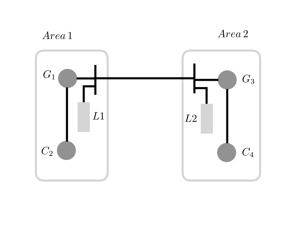
We adopt the linearized MATLAB model of Kundur’s four-machine two-area system, depicted in Figure 1, with parameters (in p.u.) from [16] and adapt it to our setup. In particular, we replace $G_{2}$ by DC/AC converter $C_{1}$ and $G_{4}$ by DC/AC converter $C_{2}$, both in closed-loop with matching control (known to have droop control properties [18]), index each machine by its area number (1 or 2), set the lines to be purely inductive, integrate continuous correlated noise with intensity $\gamma=0.05$. The initial conditions are uncorrelated and normally distributed with mean $\xi_{0}=\begin{bmatrix}93.077,69.3918,56.5361,45.6552\end{bmatrix}^{\top}$ and variance $\Sigma_{0}=\left[\begin{smallmatrix}\sqrt{0.07}\,I_{2}&0\\ 0&\sqrt{0.01}\,I_{2}\end{smallmatrix}\right]$. The assumption on negative total machines power is satisfied with $\overline{P}=-P^{*}_{G1}-P^{*}_{G2}=0.7778+0.798889=1.5767$, due to the presence of the load $L_{1}$ and $L_{2}$. This corresponds to a nominal operation for the synchronous machines $G_{1}$ and $G_{3}$ as given by [16].

We search for the optimal inertia $m_{C,i}$ (in [MW $s^{2}$/rad]) and the optimal damping $d_{C,i}$ (in [MW s/rad]), minimizing (15), with $n=4$ and $n_{C}=2$. The upper bounds on inertia and damping are given by $\overline{M_{i}}=\frac{|P_{max,i}|}{\max_{t\geq 0}|\dot{\omega}_{i}(t)|}$ and $\overline{D_{i}}=\frac{|P_{max,i}|}{\max_{t\geq 0}|\omega_{i}(t)|}$, as in [10], where we denote by $P_{max,i}$ the maximal power of the $i$-th converter. The minimal values are chosen, so that $\underline{M}_{1}=\underline{D}_{1}=10$ and $\underline{M}_{2}=\underline{D}_{2}=5$, where $m_{C,1}+m_{C,2}=120,\,d_{C,1}+d_{C,2}=40$ (in SI). By solving (15) using the algorithm from [13] and MATLAB function $\tt{fmincon}$, we arrive at the optimal inertia and damping values: $m^{*}_{C,1}=50.00139,\,m^{*}_{C,2}=69.9987$ and $d_{C,1}^{*}=5.0001$ and $d_{C,2}^{*}=34.9999$. This amounts to the $\mathcal{H}_{2}$ -norm value of $0.1630$. If we instead allocate the damping and inertia uniformly according to $\hat{m}_{C,1}=\hat{m}_{C,2}=60$ and $\hat{d}_{C,1}=\hat{d}_{C,2}=20$, then the $\mathcal{H}_{2}$ norm is $0.3217$, which agrees with our predictions from Section IV-B.

Figures 2 and 3 show the frequency response in simulations at each of the generation units, under spatially correlated noise as in (2). Frequency transients infer power system losses incurred by the generation units to return to synchrony. A synchronization at the individual areas (1 and 2) is observed at all the plots, followed by a synchronization at all generation units at the steady state frequency $\omega^{*}=1$ p.u. By comparing the subplots in Figures 2 and 3, representing the frequencies at the converters $\omega_{C,1}$ and $\omega_{C,2}$ (plotted against the frequency of the machines $\omega_{G,1}$ in Area 1 and $\omega_{G,2}$ in Area 2), the optimal allocation of inertia and damping $(m^{*}_{C,1},d^{*}_{C,1})$ at the converters $C_{1}$ and $(m^{*}_{C,2},d^{*}_{C,2})$ at the converters $C_{2}$, resulting from solving (15), allows for significantly better transients for both converters, that uniform damping and inertia gains $(\hat{m}_{C,1},\hat{d}_{C,1})=(\hat{m}_{C,2},\hat{d}_{C,2})$ does not achieve.

Starting from an SDE model for heterogeneous power networks with non-uniform inertia and damping and subject to correlated noise with random initial conditions, we examined the overall network performance by finding bounds on $\mathcal{H}_{2}$ norm. Then, for the mixed-power generation setup consisting of DC/AC converters in closed-loop with droop control and synchronous machines, we formulated different scenarios for performance optimization under the derived bounds on $\mathcal{H}_{2}$ norm. Our simulations showcase our findings for the optimal inertia and damping allocation. Future directions include the investigation of network performance for more detailed models, and the study of (approximation) solutions to the proposed optimization schemes.

The authors would like to thank Dr. Emma Tegling for the insightful comments and discussions.

References

- [1] T. Ackermann, T. Prevost, V. Vittal, A. J. Roscoe, J. Matevosyan, and N. Miller, “Paving the way: A future without inertia is closer than you think,” IEEE Power and Energy Magazine, vol. 15, no. 6, pp. 61–69, 2017.
- [2] U. Markovic, O. Stanojev, E. Vrettos, P. Aristidou, and G. Hug, “Understanding stability of low-inertia systems,” 2019.
- [3] F. Milano and R. Zárate-Miñano, “A systematic method to model power systems as stochastic differential algebraic equations,” IEEE Transactions on Power Systems, vol. 28, no. 4, pp. 4537–4544, 2013.
- [4] D. Podolsky and K. Turitsyn, “Random load fluctuations and collapse probability of a power system operating near codimension 1 saddle-node bifurcation,” in 2013 IEEE Power & Energy Society General Meeting. IEEE, 2013, pp. 1–5.
- [5] Y. Guo and T. H. Summers, “A performance and stability analysis of low-inertia power grids with stochastic system inertia,” arXiv preprint arXiv:1903.00635, 2019.
- [6] X. Chen, J. Lin, F. Liu, and Y. Song, “Optimal control of AGC systems considering non-gaussian wind power uncertainty,” IEEE Transactions on Power Systems, 2019.
- [7] G. Russo, F. Wirth, and R. Shorten, “On synchronization in continuous-time networks of nonlinear nodes with state-dependent and degenerate noise diffusion,” IEEE Transactions on Automatic Control, vol. 64, no. 1, pp. 389–395, 2018.
- [8] G. Weiss, Q.-C. Zhong, T. C. Green, and J. Liang, “H/sup/spl infin//repetitive control of DC-AC converters in microgrids,” IEEE Transactions on Power Electronics, vol. 19, no. 1, pp. 219–230, 2004.
- [9] U. Markovic, Z. Chu, P. Aristidou, and G. Hug, “LQR-based adaptive virtual synchronous machine for power systems with high inverter penetration,” IEEE Transactions on Sustainable Energy, vol. 10, no. 3, pp. 1501–1512, 2018.
- [10] B. K. Poolla, D. Groß, and F. Dörfler, “Placement and implementation of grid-forming and grid-following virtual inertia and fast frequency response,” IEEE Transactions on Power Systems, vol. 34, no. 4, pp. 3035–3046, 2019.
- [11] X. Wu, F. Dörfler, and M. R. Jovanović, “Input-output analysis and decentralized optimal control of inter-area oscillations in power systems,” IEEE Transactions on Power Systems, vol. 31, no. 3, pp. 2434–2444, 2015.
- [12] E. Tegling, B. Bamieh, and D. F. Gayme, “The price of synchrony: Evaluating the resistive losses in synchronizing power networks,” IEEE Transactions on Control of Network Systems, vol. 2, no. 3, pp. 254–266, 2015.
- [13] B. K. Poolla, S. Bolognani, and F. Dörfler, “Optimal placement of virtual inertia in power grids,” IEEE Transactions on Automatic Control, vol. 62, no. 12, pp. 6209–6220, 2017.
- [14] F. Paganini and E. Mallada, “Global analysis of synchronization performance for power systems: bridging the theory-practice gap,” IEEE Transactions on Automatic Control, 2019.
- [15] S. Curi, D. Groß, and F. Dörfler, “Control of low-inertia power grids: A model reduction approach,” in 2017 IEEE 56th Annual Conference on Decision and Control (CDC). IEEE, 2017, pp. 5708–5713.
- [16] P. Kundur, N. J. Balu, and M. G. Lauby, Power system stability and control. McGraw-hill New York, 1994, vol. 7.
- [17] J. W. Simpson-Porco, F. Dörfler, and F. Bullo, “Synchronization and power sharing for droop-controlled inverters in islanded microgrids,” Automatica, vol. 49, no. 9, pp. 2603–2611, 2013.
- [18] C. Arghir, T. Jouini, and F. Dörfler, “Grid-forming control for power converters based on matching of synchronous machines,” Automatica, vol. 95, pp. 273–282, 2018.
- [19] H. Bevrani and J. Raisch, “On virtual inertia application in power grid frequency control,” Energy Procedia, vol. 141, pp. 681–688, 2017.
- [20] F. Dorfler and F. Bullo, “Kron reduction of graphs with applications to electrical networks,” IEEE Transactions on Circuits and Systems I: Regular Papers, vol. 60, no. 1, pp. 150–163, 2012.
- [21] B. Bamieh and D. F. Gayme, “The price of synchrony: Resistive losses due to phase synchronization in power networks,” in 2013 American Control Conference. IEEE, 2013, pp. 5815–5820.
- [22] T. H. Summers, F. L. Cortesi, and J. Lygeros, “On submodularity and controllability in complex dynamical networks,” IEEE Transactions on Control of Network Systems, vol. 3, no. 1, pp. 91–101, 2015.
- [23] M. H. de Badyn and M. Mesbahi, “Growing controllable networks via whiskering and submodular optimization,” in 2016 IEEE 55th Conference on Decision and Control (CDC). IEEE, 2016, pp. 867–872.