Light- and strange-quark mass dependence of the meson revisited
Abstract
Recent lattice data on -scattering phase shifts in the vector-isovector channel, pseudoscalar meson masses and decay constants for strange-quark masses smaller or equal to the physical value allow us to study the strangeness dependence of these observables for the first time. We perform a global analysis on two kind of lattice trajectories depending on whether the sum of quark masses or the strange-quark mass is kept fixed to the physical point. The quark mass dependence of these observables is extracted from unitarized coupled-channel one-loop Chiral Perturbation Theory. This analysis guides new predictions on the meson properties over trajectories where the strange-quark mass is lighter than the physical mass, as well as on the SU(3) symmetric line. As a result, the light- and strange-quark mass dependence of the meson parameters are discussed and precise values of the Low Energy Constants present in unitarized one-loop Chiral Perturbation Theory are given. Finally, the current discrepancy between two- and three-flavor lattice results for the meson is studied.
pacs
13.75.Lb 11.30.Rd, 12.38.Gc, 14.40.-nI Introduction
The meson is the lightest vector meson in the hadron spectrum and one of the most studied hadrons in the literature. It is one of the best examples of a resonance well described within the quark model. Its phase shift fits well into a simple Breit-Wigner (BW) parameterization up to small corrections Pisut and Roos 1968; Lafferty 1993 and it is usually considered as the prototype of narrow resonance in the light-quark sector. It also dominates the scattering amplitude in the decaying almost exclusively to two pions Tanabashi et al. 2018 channel below 1 GeV,11 1 Where and refer to isospin and angular momentum, respectively. decaying almost exclusively to two pions Tanabashi et al. 2018. The -meson mass and width are well known from experiment; the Particle Data Group (PDG) quotes for their BW values and , respectively Tanabashi et al. 201822 2 These values correspond to the average value for the charged meson seen in decays and collisions. From the theory side, the most precise determination of its pole parameters comes from the Roy-equation analysis of scattering Ananthanarayan et al. 2001; Colangelo et al. 2001; Garcia-Martin et al. 2011a; Garcia-Martin et al. 2011b; Pelaez et al. 2019. The contribution of the is also important for the hadronic total cross section Aubert et al. 2009; Babusci et al. 2013; Ablikim et al. 2016, which explains applications that go well beyond low-energy meson physics, ranging from the hadronic-vacuum polarization and the light-by-light contributions to the anomalous magnetic moment of the muon (see, for instance, Eidelman and Jegerlehner 1995; Jegerlehner and Nyffeler 2009; Colangelo et al. 2017; Colangelo et al. 2019) to the electromagnetic and tensor-nucleon form factors Belushkin et al. 2007; Lorenz et al. 2015; Hoferichter et al. 2016a; Hoferichter et al. 2019. Furthermore, it also plays a crucial role in the analysis of heavy meson decays Kang et al. 2014; Niecknig and Kubis 2015 and in the restoration of chiral symmetry at high temperatures Pisarski 1995; Harada and Yamawaki 2001; Rapp et al. 2010; Gomez Nicola et al. 2013a; Gomez Nicola et al. 2013b; Gómez Nicola and Ruiz de Elvira 2016; Gomez Nicola and Ruiz de Elvira 2018; Gómez Nicola and Ruiz De Elvira 2018; Gómez Nicola et al. 2019.
Although, the -meson properties fit well within the naive quark-model picture, its nature in terms of QCD degrees of freedom is still under discussion Hu et al. 2016. Nevertheless, at low energies QCD becomes non perturbative, what hinders the study of hadron composition in terms of the fundamental QCD degrees of freedom. LatticeQCD simulations attempt to tackle this problem, however, several challenges are met when dealing with hadron scattering processes Briceño et al. 2018; Mohler 2015. In this regard, the and expansions ’t Hooft 1974; Witten 1979; Cohen et al. 201433 3 and stand for the quark mass and number of colors, respectively. provide model independent predictions to identify different kinds or hadrons. These parameters can be used to study whether the response of resonance properties to a change on or compares well with the behavior expected for different QCD configurations. For instance, by studying the dependence of the -meson properties, it was found that it also has a small non- component Pelaez and Rios 2006; Ruiz de Elvira et al. 2011; Guo et al. 2012a; Guo et al. 2012b; Ledwig et al. 2014. In addition, the analysis of the quark-mass dependence of the parameters by means of the generalization of the Feynman-Hellmann theorem for resonances suggests that it requires non-negligible corrections beyond the quark model Ruiz de Elvira et al. 2017. In this way, the extraction of the light- and strange-quark mass dependence of the -meson parameters from LatticeQCD simulations provides a powerful tool to confront quark-model predictions.
At low energies, Chiral Perturbation Theory (ChPT) Weinberg 1979; Gasser and Leutwyler 1984; Gasser and Leutwyler 1985 is the Effective Field Theory (EFT) that controls the quark-mass dependence of hadronic observables. ChPT encodes the interactions of the pseudo-Goldstone bosons of the spontaneous chiral symmetry breaking, and hence, it is capable to describe the quark-mass dependence of the light-pseudoscalar meson masses and decay constants at low energies, being these completely inherited from QCD Gasser and Leutwyler 1984; Gasser and Leutwyler 1985. Nevertheless, ChPT is constructed as an expansion in quark masses and momenta and hence it is only valid below a certain scale. Therefore, ChPT does not provide direct information about resonance properties. On the contrary, unitarized Chiral Perturbation Theories (UChPTs) Truong 1988; Dobado et al. 1990; Dobado and Pelaez 1993; Dobado and Pelaez 1997; Nieves and Ruiz Arriola 1999; Oller et al. 1999; Nieves and Ruiz Arriola 2000; Gomez Nicola and Pelaez 2002 are based on imposing exact unitarity while matching ChPT at low energies. Thus, the region of validity of the chiral expansion is extended, allowing one to generate poles on unphysical Riemann sheets in the complex-energy plane and to access resonance properties. In particular, the Inverse Amplitude Method (IAM) Truong 1988; Dobado et al. 1990; Dobado and Pelaez 1993; Dobado and Pelaez 1997 generates the resonance from scattering and provides a tool to study the light- and strange-quark mass dependence of the -meson properties, while reproducing the chiral series at low energies. Thus, in this work we utilize the IAM to investigate the quark mass dependence of the -meson pole parameters, such as its mass, width and couplings to the and channels. The analysis of these properties requires the determination of the Low Energy Constants (LECs) involved in the pseudoscalar meson masses, decay constants and meson-meson scattering. A chiral trajectory specifies the way in which the light- and strange-quark masses vary. In UChPT, the behavior of resonance properties over chiral trajectories is controlled by chiral symmetry and unitarity. It is desired to determine LECs which provide a full description of the resonance properties on chiral trajectories where and/or vary. These kind of predictions of an EFT can be tested by lattice QCD simulations.
LatticeQCD (LQCD) is the only known tool to extract non-perturbative information from QCD. It is the instrument to determine the low-energy parameters of the chiral Lagrangian that govern the quark mass dependence of resonance properties, hence, rendering evidence of the EFT predictions. In recent simulations, lattice data on scattering have been extracted for several pion masses for two light flavors () Aoki et al. 2007; Gockeler et al. 2008; Feng et al. 2011; Lang et al. 2011; Pelissier and Alexandru 2013; Bali et al. 2016; Guo et al. 2016; Erben et al. 2020; Fischer et al. 2020 and including also the strange quark () Wilson et al. 2015; Dudek et al. 2013; Bulava et al. 2016; Feng et al. 2015; Alexandrou et al. 2017; Fu and Wang 2016; Metivet 2015. See also Werner et al. 2020; Miller et al. 2020 for recent simulations. Surprisingly, results for the mass in simulations are at odds with experimental predictions. Namely, the simulation with the lightest pion mass MeV by the RQCD Collaboration Bali et al. 2016 predicts a -meson mass around MeV below the physical value Bali et al. 2016. Other simulations also show disagreement with the closest pion-mass result for . For example, the GWU simulation at MeV Guo et al. 2016 gives a -meson mass around MeV lighter than the Hadron Spectrum (HadSpec) outcome of the simulation for MeV Wilson et al. 2015. It has been argued in recent analyses Guo et al. 2016; Hu et al. 2016 with the UChPT model of Oller et al. 1999, that this difference can be explained through the effect of loops in the reaction, where the kaon is off-shell. This effect has been shown to be consistent among the simulations Hu et al. 2016. Moreover, while the error ellipses of lattice data analyses do overlap, hence showing consistency among the simulations, the same cannot be stated for the results, where one finds inconsistencies among lattice simulations Hu et al. 2016.
The light-quark mass dependence on decay constants has also been studied in LQCD simulations in Bruno et al. 2017; Blum et al. 2016; Bazavov et al. 2010a; Bazavov et al. 2010b; Aubin et al. 2008; Noaki et al. 2009; Aoki et al. 2009; Baron et al. 2010. However, almost no attention has been paid in the past to their strange–quark-mass dependence, nor of the phase shift. Most of these simulations have been performed with a strange-quark mass kept fixed at the physical point, .44 4 The superscript “0” stands for physical point from now on. A reflection of this can be found in the Flag Review Aoki et al. 2019; the averaged LEC values from different fits to decay constants with ChPT do not represent a global analysis of data and they do not track other trajectories rather than those with roughly . In addition, these LECs do not describe the meson-meson interaction at the energies where the meson begins to resonate. The only exception up to recently was a simulation of the pion decay constant done by MILC over the trajectory Bazavov et al. 2010a. Thus, in spite of the great advance of lattice simulations, data out of the chiral trajectory are still scarce, even though the response of hadron properties to different chiral trajectories could elucidate their strangeness nature, in particular, and dynamical nature, in general. A larger amount of highly precise data on a variety of chiral trajectories are necessary to shed light on the composition of hadrons.
Recently, the CLS Collaboration generated ensembles on different chiral trajectories with , (where and denotes a constant), in large volumes Andersen et al. 2019; Bruno et al. 2017. Moreover, this constant varies a little with the inverse gauge coupling, , of the simulation, which characterizes the set of ensembles generated. These trajectories are of particular interest since the hadron response along the trajectory will manifest as a consequence of both, variations in the light and strange quarks. These recent lattice simulations motivate the present analysis by investigating them in combination with the simulations over trajectories. This provides a good ground to study the strange-quark mass dependence of decay constants and the phase shift, which we intend to do here. Of course, new LQCD simulations over trajectories with larger variations on these constants or for different values of the strange-quark mass in the trajectories would improve the analysis presented here.
The study of hadron properties ( meson) we conduct here needs to emphasize the role of pseudoscalar decay constants, which are strongly connected to the coupling of vector mesons to pions. This is supported by the assumption of dominance of vector mesons in the pion-photon coupling, the so-called Vector Meson Dominance (VMD) Sakurai 1969, which connects the size of the pion decay constant () and the coupling () in the EFT Birse 1996. In this context, the large experimentally observed decay width of the meson is directly connected to its coupling to two pions, which explains why the -meson phase shift and -meson properties are tightly related to the size of . In this sense, these two observables should always be determined together in lattice simulations. Beyond that, the quark mass dependence of pseudoscalar decay constants fixes the chiral trajectories in the lattice and hence, they can be used to set the lattice scale by letting them go to the physical point.
The analysis we perform here will be useful to further check the KSFR relation Riazuddin and Fayyazuddin 1966, which under VMD states that in the SU(3) limit where . While, it is common that in previous lattice/experimental data analyses of -meson phase shift the -meson mass increases monotonically with , so that the KSFR relation is fulfilled Hanhart et al. 2008; Pelaez and Rios 2010; Nebreda and Pelaez. 2010; Guo et al. 2016; Hu et al. 2017, this behavior was not observed in the recent data of Andersen et al. 2019. Whether this is a consequence of the lightness of the strange-quark mass used in these simulations or not will also be checked in the present analysis.
In conclusion, we analyze here the lattice data on -meson phase shifts in of Dudek et al. 2013; Wilson et al. 2015; Bulava et al. 2016; Andersen et al. 2019, in combination with decay constant lattice data from Bruno et al. 2017; Blum et al. 2016; Bazavov et al. 2010a; Bazavov et al. 2010b; Aubin et al. 2008. Moreover, the lattice data of Feng et al. 2015; Alexandrou et al. 2017; Noaki et al. 2009; Aoki et al. 2009 are also considered in separated analyses.
Let us make some initial remarks. Experimental phase-shift data on scattering in the channel were successfully reproduced using the IAM Gomez Nicola and Pelaez 2002; Hanhart et al. 2008; Pelaez and Rios 2010; Nebreda and Pelaez. 2010. Here, the LECs are extracted by performing a fit to lattice phase-shift data instead, taking into account the covariance matrix for energy levels, similarly as in Hu et al. 2017. The main differences with the work of Hu et al. 2017 are:
- 1.
A global fit to lattice data on two distinct chiral trajectories, and , is done instead of considering trajectories only over simulations.55 5 Here, or , where only data on are included in the latter Bazavov et al. 2010a. As mentioned previously, this includes data from Andersen et al. 2019; Bruno et al. 2017 for and from Dudek et al. 2013; Wilson et al. 2015; Bulava et al. 2016; Blum et al. 2016; Bazavov et al. 2010a; Bazavov et al. 2010b; Aubin et al. 2008 for .
- 2.
We perform a simultaneous fit of phase shift and decay constant lattice data. Note that in Hu et al. 2017, only phase-shift data were analyzed, while the quark mass behavior of pseudoscalar decay constants was fixed with the LECs obtained in the fit done in Nebreda and Pelaez. 2010, which only included lattice data on .
- 3.
The theoretical framework used here is the IAM in coupled channels Gomez Nicola and Pelaez 2002 instead of the simplified UChPT model considered in Oller et al. 1999, which was taken into account in Hu et al. 2017. This is, we include here one-loop diagrams not just in the channel, but also in the and channels, hence, consistently with chiral symmetry at low energies.
- 4.
For the CLS data in Andersen et al. 2019; Bruno et al. 2017 the systematic error in the lattice spacing is taken into account in the final fit by using the bootstrap method, assuming that the lattice spacing is normally distributed with the standard deviation associated to the lattice error.
Although in the present analysis we only include lattice data, this work can be considered as complementary to the previous and analyses done in Hanhart et al. 2008; Pelaez and Rios 2010; Guo et al. 2016; Hu et al. 2016 and Nebreda and Pelaez. 2010; Hu et al. 2017, respectively, or to the recent two-loop IAM study in Niehus et al. 2020. If the strange-quark mass has no effect on the -meson properties extracted from the lattice simulations, then, the disagreement among and lattice results will be due to the scale setting or other finite volume effects, such as the lattice spacing or the box size. Thus, we study in detail in which particular quark-mass regime the -meson properties in the simulation are sensitive to both, the strange- and light -, -quark masses.
This paper is organized as follows. In section II we explain the formalism considered. In section III, we show the results of a global analysis on decay constants over several chiral trajectories. Section IV provides the results of the combined fit both to phase shift and decay constant lattice data. In particular, we first analyze in IV.1 lattice data over trajectories, while the same analyses for the data are shown in section IV.2. Following this, we present our final results on a global fit on both trajectories in section V. Finally, the main conclusions are presented in section VI.
II Theoretical framework
II.1 Chiral Perturbation Theory
At low energies QCD interactions become non-perturbative and EFTs provide the proper framework to perform systematic calculations. The basic premise of EFTs is that the dynamics at low energies (or large distances) do not depend on the details of the dynamics at high energies (or short distances). As a result, low-energy hadron physics can be described using an effective Lagrangian containing only a few degrees of freedom, hence, ignoring those present at higher energy scales.
Chiral perturbation theory is the low-energy EFT of QCD. It is built as the most general expansion in terms of derivatives and quark masses Gasser and Leutwyler 1984; Gasser and Leutwyler 1985 compatible with QCD symmetries, which relevant degrees of freedom at low energies are the pseudo Nambu–Goldstone bosons (NGB) of the chiral symmetry spontaneous breakdown, i.e., pion, kaon and eta mesons.
At leading order (LO) in this expansion, the chiral Lagrangian reads
| (1) |
where coincides with the pion decay constant in the chiral limit and , with a constant to be related with the quark condensate and is the three-flavor quark-mass matrix, where exact isospin symmetry is assumed. The matrix collects the contribution of pions, kaons and etas, with
By expanding the LO chiral Lagrangian in powers of , one can identify the mass field terms obtained with the pseudo NGB fields, which yields a relation between meson and quark masses
| (5) |
The constant is related with the quark condensate value in the chiral limit,
| (6) |
with , leading to the well known Gell–Mann–Oakes-Renner formula Gell-Mann et al. 1968, i.e., even though both and are scale dependent quantities, and hence, they are not observables, their product is scale independent.
At higher orders, all terms in the Lagrangian come multiplied by LECs, which contain information about higher energy scales. In addition, they absorb the divergences which appear in the chiral expansion, so that, the theory is renormalizable order by order. Unfortunately, the LECs cannot be determined perturbatively from QCD. While the LECs which multiply energy-dependent terms can be extracted quite well from dispersion theory Bijnens and Jemos 2012; Bijnens and Ecker 2014; Hoferichter et al. 2015a; Siemens et al. 2017, Lattice QCD provides in principle a model independent way to determine the values of LECs which fix the quark mass dependence Leutwyler 2015; Aoki et al. 2019.
The NLO Lagrangian was first derived in Gasser and Leutwyler 1984 for two flavors. The effect of the strange quark was studied in Gasser and Leutwyler 1985. Omitting field tensor and vacuum terms, the SU(3) NLO ChPT Lagrangian reads
| (7) |
In Eq. (II.1), , and multiply massless terms and hence they also contribute in the chiral limit. and accompany terms depending linearly on the quark masses and they contribute to the renormalization of the NGB wave functions and decay constants. Lastly, , and come together with quadratic terms on the quark mass. These only contribute to the renormalization of the NGB masses and have a minor role in the determination of the meson properties.
One-loop correction to the pion, kaon and eta NGB masses read Gasser and Leutwyler 1985
| (8) | ||||
| (9) |
| (10) |
with
| (11) |
The superscript denotes renormalized LECs, which carry the dependence on the regularization scale Gasser and Leutwyler 1985. This scale dependence cancels exactly in the calculation of any observable. In the following, we will identify the physical NGB masses with the one-loop ChPT prediction above. Nevertheless, note that the quark mass dependence is always expressed in terms of the leading order NGB masses.
In addition, while at LO the NGB decay constant is independent of the quark mass, one-loop corrections in the pseudoscalar decay constants lead to
| (12) | ||||
| (13) | ||||
| (14) |
which are also identified with the physical quantities.
II.2 Meson-meson scattering in ChPT
The scattering of NGB meson is computed in ChPT as an expansion in momenta and meson masses. Denoting as the scattering amplitude of the NGB process with defined isospin , one has the generic form
| (15) |
where , and are the usual Mandelstam variables and , where means either meson momenta or masses. The LO amplitude is obtained at tree level from the Lagrangian. The NLO contribution contains one-loop diagrams from plus tree-level contribution from involving LECs.
The scattering amplitude at one-loop order in ChPT was computed first in Gasser and Leutwyler 1984 in a two-flavor formalism and in Gasser and Leutwyler 1985 for three flavors. The and scattering amplitudes were evaluated in Bernard et al. 1991a; Bernard et al. 1991b and Bernard et al. 1991c, respectively. The one-loop expressions for the SU(3) pseudo NGB reactions used here can be found in Gomez Nicola and Pelaez 2002. The SU(2) and SU(3) two-loop scattering amplitudes were obtained in Knecht et al. 1995; Bijnens et al. 1996 and Bijnens et al. 2004a, respectively. The two-loop amplitude was determined in Bijnens et al. 2004b. Recently, first three-loop calculations have been explored in Bijnens et al. 2019.
Using the normalization conventions given in Gomez Nicola et al. 2010; Ruiz de Elvira and Ruiz Arriola 2018, the -channel partial-wave projection of the amplitude is defined as
| (16) |
where is a normalization factor equal to if all the particles are identical and otherwise. The Mandelstam variables and are defined by the kinematics of the corresponding process and , being the scattering angle in the center-of-mass frame.
Being an expansion in momenta and masses, it is clear that ChPT cannot satisfy unitarity, which in the elastic case implies the relation
| (17) |
where and is the momentum in the center-of-mass frame. In the following, we only consider the channel and the superscript index will be suppressed to ease the notation. Nevertheless, ChPT satisfies elastic unitarity perturbatively. For instance, defining as
| (18) |
the chiral series of the partial-wave amplitude, with and the tree-level and one-loop ChPT partial-wave amplitudes, in the elastic case one finds the relations
| , | (19) |
which implies that the unitarity bound in Eq. (17) is increasingly violated in ChPT at larger energy values. In practice, it implies that the chiral series is limited to scattering momenta around 200 MeV above threshold. Furthermore, the ChPT series does not converge equally well in all parts of the low-energy region. This is particularly evident in the scalar-isoscalar channel where strong pion-pion rescattering effects slow the convergence of the chiral series Meißner 1991. Finally, at increasingly large momenta, several partial-waves become resonant. Resonances are non-perturbative effects and, as such, they cannot be reproduced within the ChPT power expansion. Furthermore, they usually saturate the unitarity bound in Eq. (17), which implies that elastic unitarity can be violated in the resonance region.
II.3 Unitarity and analyticity
Below the four-pion production threshold, located at , scattering is purely elastic and, consequently, it can be described in terms of its phase shift. Above this energy, there are possible intermediate processes such as , with or , which, in principle, have to be taken into account. In our case of interest, the -wave -scattering partial wave, inelasticities are completely negligible below the threshold and very small below 1.4 GeV Protopopescu et al. 1973; Hyams et al. 1973; Grayer et al. 1974; Estabrooks and Martin 1974; Garcia-Martin et al. 2011a; Pelaez et al. 2019; Navarro Pérez et al. 2015. Thus, in this work elastic scattering is assumed to occur below the threshold and above only the and channels are considered.
The unitarity condition for the -matrix, , implies that, for two-coupled channels, it can be parameterized in terms of only three independent parameters. It is customary to choose them as the and phase shifts, denoted as as and , respectively, and the inelasticity . Thus, the S-matrix is expressed as
| (20) |
The -matrix elements of the scattering amplitude are related to -matrix elements as,
| (21) |
with
and . The relation between the - and -matrix, Eq. (21), allows one to derive the following unitarity condition for the -matrix elements
| (24) |
or
| (25) |
in matrix form, being
| (26) |
Eq. (25) implies the coupled-channel unitarity relation
| (27) |
is fulfilled. The phase space definition, Eq. (II.3), ensures that in the elastic case, i.e., below the threshold, elastic unitarity is satisfied. In the one channel case, Eq. (27) simplifies to
| (28) |
The unitarity conditions in Eqs. (27) and (28) imply that the inverse of the imaginary part of an scattering amplitude in the physical region is completely fixed by unitarity. The strong relation between unitarity and resonances has motivated the development of several ChPT inspired methods based on imposing exact unitarity. Some of them are the so-called -matrix method Gupta 1977 and the chiral unitarity approach. The latter was considered first in Oller and Oset 1997; Oller et al. 1999 to describe and scattering in the scalar-isoscalar channel, leading to fairly precise determinations of the and resonance properties. There are also more involved unitarization methods. For example, the Bethe-Salpeter (BS) equations were solved for scattering in Nieves and Ruiz Arriola 1999; Nieves and Ruiz Arriola 2000, both in the on-shell and off-shell schemes, while the N/D method was employed in Oller and Oset 1999 providing also results for the rest of lightest scalars, namely the and . However, none of them generates the pole in the scattering wave.
The energy-dependence of an scattering amplitude is also strongly constrained by analyticity. Analyticity is based on the Mandelstam hypothesis Mandelstam 1959, i.e., the assumption that an scattering amplitude is represented by a complex function that presents no further singularities than those required by general principles such as unitarity and crossing symmetry. In this way, poles in the real axis are associated with bound states (absent in low-energy meson-meson scattering) and production thresholds give rise to cuts. Cuts are a consequence of the unitarity condition given in Eq. (25), which, together with the Schwartz-reflection principle, imply that an scattering amplitude must have a cut where unitarity demands its imaginary part to be non-zero. It occurs due to both, direct and crossed channels, leading to a right- (RHC) and left-hand cut (LHC), respectively.
Once analyticity is established, Cauchy’s integral formula allows one to construct a representation that relates the amplitude at an arbitrary point in the complex plane to an integral over its imaginary part along the right- and left-hand cuts, the so called dispersion relations. The convergence of the dispersive integral often requires subtractions, which introduce a certain number of a priori undetermined constants. The Froissart–Martin bound Froissart 1961; Martin 1963 guarantees that at most two subtractions are needed to ensure the convergence at infinity, but one subtraction is enough for the scattering amplitude in the vector-isovector channel. Thus, a once-subtracted dispersion relation for scattering reads
| (29) |
where the first and second integrals stand for the RHC and LHC contributions, respectively. The subtraction constants involve the evaluation of the amplitude at , so that, they can be pinned down by matching to ChPT in the regime where the chiral expansion is expected to show better convergence properties. However, while the value of in the physical RHC is constrained from unitarity, the LHC contribution is in principle unknown. On the one hand, most UChPT methods differ in the way the LHC is treated. While the -matrix and chiral unitarity approach models simply neglect the LHC contribution, the BS and N/D methods approximate it with ChPT. On the other hand, Roy–Steiner equations Roy 1971; Hite and Steiner 1973 solve this problem exactly using crossing symmetry. They provide a representation involving only the physical region, but which, at the same time, intertwines all partial-waves with different isospin and angular momentum. Although, Roy–Steiner-equation solutions allow for high-precision descriptions of different scattering processes at low energies Ananthanarayan et al. 2001; Colangelo et al. 2001; Garcia-Martin et al. 2011a; Buettiker et al. 2004; Hoferichter et al. 2016b, and provide the proper framework to extract resonance pole parameters Caprini et al. 2006; Descotes-Genon and Moussallam 2006; Garcia-Martin et al. 2011b; Masjuan et al. 2014; Caprini et al. 2016; Peláez et al. 2017, or to evaluate an scattering amplitude in an unphysical region Hoferichter et al. 2015b; Hoferichter et al. 2016c; Ruiz de Elvira et al. 2018, their analysis requires experimental information for the high-energy contribution and higher partial waves. Thus, they are in principle inappropriate for the analysis of lattice data at different quark masses. In this article, we follow the IAM, which will be outlined in the next section II.4.
II.4 Elastic Inverse Amplitude Method
The Inverse Amplitude Method exploits the relation between a dispersion relation for the inverse of an scattering amplitude and the ChPT amplitude at a given order. At NLO in the chiral expansion, taking into account that ChPT amplitudes grow as when , one needs three subtractions to ensure the convergence at high energies. Thus, a thrice-subtracted dispersion relation for a elastic ChPT -scattering partial wave reads
| (30) |
where we have used Eq. (II.2) to fix the absorptive part of in the physical region. Note that Eq. (II.4) is strongly related to a thrice subtracted dispersion relation for the function ,
| (31) |
so that in an elastic approximation the RHC contribution coincides exactly with that of . The subtraction constants require the evaluation of the scattering amplitude and its derivatives at , the kinematic region where ChPT provides a reliable description. Thus, using ChPT at NLO one gets
| (32) | ||||
Being the RHC exactly fixed from unitarity, and once the subtraction constants are estimated using ChPT, the only remaining unknown information in Eq. (II.4) is the LHC. The left-hand cut might indeed play a relevant role below threshold, but it is expected that its contribution should be less important as one moves into the physical region. Thus, for a qualitative description it is sufficient to approximate the left-hand cut using ChPT. At NLO, one finds
| (33) |
Inserting Eqs. (32) and (33) in Eq. II.4 one obtains
| (34) |
which stands for the well-known equation of the IAM method. The IAM was derived first in Truong 1988; Dobado et al. 1990 using only unitarity for scattering. Its derivation from a dispersion relation and application thereafter to scattering was investigated in Dobado and Pelaez 1993; Dobado and Pelaez 1997, whereas the remaining IAM meson-meson scattering processes were studied in Gomez Nicola and Pelaez 2002 to one loop. The two-loop version of the IAM was derived in Nieves et al. 2002 and its generalization to include the effect of Adler zeros was obtained in Gomez Nicola et al. 2008.
The IAM provides a simple algebraic equation that ensures elastic unitarity while at low energies reproduces the chiral expansion. This fact implies that the IAM can be used to describe the resonance region below 1 GeV, i.e., well beyond the applicability range of ChPT. Furthermore, it is based on a dispersion relation, hence, its use in the complex plane is justified, providing a simple tool to study resonance properties. The main difference between the IAM and the on-shell BS or N/D method, is that, in the IAM only the absorptive part of the left-hand contribution is expanded at low energies. It implies that the left-hand cut energy dependence is still controlled by a dispersion relation instead of being fully given by ChPT. In addition, the IAM generates not only scalar but also vector resonances Oller et al. 1999, without involving new additional parameters rather than the ChPT LECs. Hence, it reproduces at low energies the quark mass dependence predicted by ChPT.
Nevertheless, it has also several caveats. While the RHC is solved exactly using elastic unitarity, the LHC is approximated using ChPT. The direct consequence of this fact is that the IAM breaks crossing symmetry. Besides, while the IAM provides higher order ChPT contributions needed to fulfill unitarity, some of the leading order logarithms from higher-order loop graphs appear with the wrong coefficients Gasser and Meißner 1991.
In addition, it is worth mentioning that the IAM describes experimental data, including resonance pole parameters, of meson-meson scattering in the region below 1 GeV only within a 10%-15% accuracy Gomez Nicola and Pelaez 2002; Pelaez 2004. This small difference highlights the relevance of the LHC in the physical region below 1 GeV.
Clearly, leaving the LECs as free parameters to be adjusted to data instead of being fixed to the ChPT values improves the description of the experimental data. Indeed, and scattering experimental data were described in Gomez Nicola and Pelaez 2002; Nebreda and Pelaez. 2010 using the IAM with LEC values compatible with pure ChPT determinations. Small LECs changes are indeed expected since the IAM includes contributions that go beyond the pure chiral expansion at a given order. However, it is important to remark that while ChPT is a natural theory in the sense that its predictions are linear in LECs changes, the IAM as well as other UChPT models are strongly dependent on precise LECs determinations. Small changes on the LEC values might produce large effects on the phase-shift and pole parameter predictions.
Finally, let us remark that the dispersive derivation of the IAM only constrains its energy dependence, and hence, it is not clear whether it provides the correct quark-mass dependence. While the IAM reproduces the ChPT series at low energies, thus, ensuring that it provides the quark-mass dependence predicted from QCD close to the chiral limit, it also introduces higher-order contributions that spoil the chiral series at higher energies and for heavier quark masses. Thus, high quality lattice data for different light- and strange-quark masses are key to ensure that the chiral extrapolation performed within the IAM is well consistent with QCD.
II.5 Coupled channel formalism
The generalization of the inverse amplitude method to coupled channels should be in principle straightforward if one assumes the factorization of the RHC and LHC contribution for the different channels involved. In this case, we can define the matrix version of the function in Eq. (II.4) as , where stands for the ChPT matrix (see Eq. (26)). Similarly as in Eq. (II.4), a thrice-subtracted dispersion relation for reads
| (35) |
where and stand for the corresponding right- and left-hand cut branching points, respectively. The numerator of the RHC contribution corresponds to the matrix version of Eq. (II.2), i.e.,
| (36) |
and hence, the right-hand cut of G(s) coincides with that of the matrix . The subtraction constants can be evaluated using ChPT. By means of expanding as
| (37) |
one recovers the equivalent version of Eq. (32) in matrix form. However, the problem now is the evaluation of the left-hand cut. Although the RHC branching point is common for all the elements of the T-matrix, the LHCs of the various channels do differ. Namely, while the scattering LHC starts at , the LHC for the partial wave opens at . In this way, proceeding as we did for the elastic IAM, i.e., taking the perturbative expansion in Eq. (37) for the absorptive part of along the LHC, one is indeed mixing the LHCs of all T-matrix elements. This translates into a violation of the factorization hypothesis, which produces spurious left-hand cuts breaking unitarity Iagolnitzer et al. 1973; Badalian et al. 1982; Guerrero and Oller 1999; Gomez Nicola and Pelaez 2002; Ledwig et al. 2014. As a summary, the analogous of Eq. (34) cannot be derived in coupled-channels using a dispersion relation.
Alternatively, one can still exploit unitarity in order to derive a coupled channel version of Eq. (34) valid in the real axis. Taking into account Eq. (27), , one can write
| (38) |
Now, can be approximated once more with ChPT. Using Eq. (37) one gets
| (39) |
which provides the IAM coupled channel unitarization formula. Note that to derive Eq. (39) we have used Eq. (36). Nevertheless, it is important to note that Eq. (39) is only justified in the real axis where the ChPT coupled channel unitarity relation (36) is fulfilled.
At this point, it is also important to discuss at which energy the couple-channel formalism should be taken into account. Given the phase-space definition in Eqs. (II.3) and (26), the unitarity relation in Eq. (25) acquires dimension two only when one crosses the production threshold. Thus, Eq. (39) should be used only above the threshold, i.e., when its dimension coincides with the number of states accessible and the coupled-channel unitarity relation in Eq. (27) is fulfilled. Below this energy one should consider the one-dimensional IAM equation. Thus, this procedure yields a discontinuity at , instead of a single continuous function. Alternatively, one can include the channel for all energies. This provides a continuous function but it again introduces spurious left-hand cuts, leading to a violation of unitarity. Nevertheless, these violations are in general small, around 2%-5% Guerrero and Oller 1999; Gomez Nicola and Pelaez 2002. In this paper we consider the second approach for Eq. (39), but in order to reduce the effect of spurious cuts, we introduce an extra term in the of our fit to lattice data, which penalizes unitarity violations of the S-matrix by some factor, as explained in Sect. II.8.
Eq. (39) was used in Gomez Nicola and Pelaez 2002 to study all possible amplitudes for meson-meson scattering leading to a fairly good description of all available experimental data below GeV with reasonable LEC values. These amplitudes were analytically continued to the complex plane in order to look for poles associated to the lightest scalar and vector resonances Pelaez and Gomez Nicola 2003; Pelaez 2004, with determinations compatible with experimental values within uncertainties. This result suggests that the role of spurious LHCs which prevent the dispersive derivation of the coupled-channel IAM formula are also small. Furthermore, we have explicitly checked that by removing the - and -channel loop functions (Fig. 1) in the and ChPT amplitudes that generate the spurious cuts, the mass and width of the -meson obtained in the global Fit IV (see Sect. V) change less than 1 and 6 MeV, respectively, i.e., within the uncertainties quoted. Nevertheless, the effect of the and channels in the amplitude lead to a shift of 6 and 15 MeV for the mass and width of the -meson in Fit IV, respectively (without readjusting the LECs).
To conclude, Eq. (39) is the tool we use to analyze lattice scattering data in the channel. The explicit expressions for the elements of the and for , and are given in the appendix of Gomez Nicola and Pelaez 2002.
II.6 Resonances
Resonances are formally defined as poles lying on unphysical Riemann sheets. An unphysical Riemann sheet is reached when the physical right-hand cut is crossed continuously from the upper-half plane to the lower-half plane above a given production threshold. In the elastic scattering case, there are only two Riemann sheets, the physical and unphysical one, which are called, first and second sheet, respectively. These two Riemann sheets must coincide in the real axis,
| (40) |
In addition, the scattering amplitude on the first Riemann-sheet satisfies the Schwartz reflection principle, i.e., , which together with unitarity, , yields the relation
| (41) |
The analytic continuation of Eq. (41) into the complex plane implies that a pole on the second Riemann sheet corresponds to a zero in the physical one. By means of Eq. (21) one can translate this relation to the -matrix elements, leading to
| (42) |
where , and its determination is chosen as , to ensure the Schwartz reflection symmetry.
When further channels are opened, more unphysical Riemann sheets can be defined by continuing the square momenta of the intermediate states over the different thresholds. Thus, there are Riemann-sheets for a given number of opened channels. The generalization of Eq. (42) in a coupled-channel formalism is straightforward
| (43) |
where is a diagonal matrix containing the phase space factors of those channels that have been crossed continuously. In particular, for the and coupled-channel case, we will have four different Riemann sheets defined as
where and are the phase space factors of the an channels, respectively.
Therefore, a pole in the matrix corresponds to a zero of the determinant of the matrix inside the brackets of Eq. (43), which is denoted by , where M and stand for the mass and width of the resonance, respectively.
In addition, the dynamics of a resonance is strongly related to its coupling to a given channel, which is defined from the pole residue as
| (45) |
where stands for the center-of-mass-system momentum of the corresponding process.
II.7 Formalism in the finite volume
The Lüscher’s approach Luscher 1986; Luscher 1991 allows one to relate the measured discrete value of the energy in a finite volume to the scattering phase shift at the same energy in the continuum. The volume-dependence of the discrete spectrum of the lattice QCD gives the energy dependence of the scattering phase shift. This method, originally derived for a single scattering process was soon extended to coupled channels for potential scattering Liu et al. 2006, non-relativistic effective theories Bernard et al. 2008; Lage et al. 2009 and to relativistic scattering Hansen and Sharpe 2012; Briceño and Davoudi 2013; Li and Liu 2013; Guo et al. 2013. Extensions of the Lüscher formalism to three-particle systems under certain conditions are also available, see for instance Polejaeva and Rusetsky 2012; Hansen and Sharpe 2014; Briceño et al. 2017; Mai and Döring 2017; Döring et al. 2018; Hansen and Sharpe 2019; Blanton et al. 2019; Pang et al. 2019; Briceño et al. 2019; Romero-López et al. 2019; Hansen et al. 2020 and references therein.
The Lüscher’s approach is based on the analysis of the dominant power-law volume dependence that enters through the momentum sums in a BS equation, where all quantities are written in terms of non-perturbative correlation functions. In order to extract this dependence one assumes that the BS kernel, which accounts for the LHC and subtraction constant contributions in Eq. (II.3) and only involves a exponentially suppressed dependence on the volume Luscher 1986, coincides for large volumes with its infinite-volume form. In this way, the difference between finite- and infinite-volume integrals entering on the BS equations only depends on on-shell values of the two-particle integrand leading to the the quantization condition66 6 Actually, in its relativist extension, Lüscher’s formulation neglects the volume dependence of the propagator dressing function or, equivalently, the real part of the two-particle propagator, which might lead to significant corrections for small volumes Chen and Oset 2013.
| (46) |
where is the scattering amplitude in the continuum and is a matrix that contains sums of the generalized Zeta functions subduced into the relevant finite volume little groups Hansen and Sharpe 2012; Briceño and Davoudi 2013.
Lüscher’s method was subsequently rederived in Döring et al. 2011; Döring et al. 2012 by discretizing the -channel loop functions which appear in the IAM coupled-channel equation of Eq. (39) and neglecting the - and -channel contributions. The discretization of the and channels has been discussed in Albaladejo et al. 2012; Albaladejo et al. 2013. In the latter, the exponentially suppressed volume dependence of the LHC contribution was explicitly taken into account, concluding that the LHC volume dependence is numerically negligible for lattice sizes while for lattice volumes , it only affects noticeably the first energy level. Furthermore, note that neglecting the volume dependence of the LHC contribution in the finite volume is by no means equivalent to ignoring the LHC in the continuum; lattice energy levels are non-perturbative quantities and, as such, they include all physical effects, both from the RHC and LHC contributions. The same cannot be stated for the dispersive formalism defined in Sect. II.4 and II.5 since one explicitly factorizes the RHC and LHC contributions. However, to extract information from the energy levels and connect them with the T-matrix in the continuum one does need a generalized Lüscher method including all physical effects, which might become particularly difficult, for example, in the case of multi-channel and intermediate states of three or more particles.
In principle, one could use the formalism in Albaladejo et al. 2012; Albaladejo et al. 2013 to evaluate the energy levels and fit them to the lattice data. Nevertheless, in order to avoid the discretization of loops we follow here the method used in Hu et al. 2017. Namely, we fit the phase shift values extracted from the lattice using Lüscher’s method, while the eigenenergies are reconstructed by means of a Taylor expansion taking into account the correlation between energy and phase shift , as well as the covariance matrix of eigenenergies provided by the lattice. This method is explained in the subsection below.
II.8 Fitting procedure
The low energy constants of SU(3) Chiral Perturbation Theory to one loop are extracted from fits to lattice phase-shift data in the channel together with pseudoscalar meson decay constants and masses. This includes the phase-shift data of Andersen et al. 2019; Dudek et al. 2013; Wilson et al. 2015; Bulava et al. 2016; Feng et al. 2015; Alexandrou et al. 2017 together with data from Bruno et al. 2017; Blum et al. 2016; Bazavov et al. 2010a; Bazavov et al. 2010b; Aubin et al. 2008; Noaki et al. 2009; Aoki et al. 2009 for decay constants.
We analyze lattice simulations on two different chiral trajectories, where either the sum of the three-lightest quarks or the strange-quark mass is fixed to the physical point, i.e., or , respectively. The corresponding tree-level pseudoscalar meson masses relations are
| (47) |
for and
| (48) |
for , with or .
As a result from a combined analysis of data on these two kind of trajectories, in Sect. V we also show predictions for -meson phase shifts, pseudoscalar meson decay constants and masses in other trajectories where the strange-quark mass is fixed to values smaller than the physical one, with , on the SU(3) symmetric trajectory, , i.e.,
| (49) |
and for trajectories where the light-quark mass is kept fixed at the physical point , i.e.,
| (50) |
We employ one-loop ChPT for the analysis of pseudoscalar meson masses and decay constants, see Sect. III, in combination with the coupled-channel IAM discussed in Sect. II.5 for the -meson phase shifts. The fitting parameters are the LECs entering into our expressions, i.e., , with , , and the parameters which fix the chiral trajectories in Eqs. (47) and (48), and . The chiral scale is fixed to MeV and the pion decay constant in the chiral limit is set to MeV. We fixed because its inclusion as a new fitting parameter did not entail any substantial reduction of the . In the following we describe the contributions to the .
Meson-meson scattering in the lattice translates into discrete energies which are correlated. In order to take into account those the following function is minimized,
| (51) |
where is the vector of eigenenergies measured on the lattice, their covariance matrix and the corresponding energies of the fit function.
Nevertheless, we do not fit directly lattice energy levels but phase shifts extracted using the Lüscher formula. In order to take into account the energy correlations, we follow the method considered in Hu et al. 2017. This is, for each energy level , , a Taylor expansion of both, the phase shift extracted from the lattice, , and the one evaluated in the IAM, , is performed around the energy given by the lattice simulation, . If one assumes that both and coincide exactly at , at leading order, one finds
| (52) |
which provides a direct way to evaluate in Eq. (51) in terms of phase shift values. The minimization of Eq. (51) allows one to avoid dealing with the generalized Zeta functions encoded in the Lüscher quantization condition. This makes the fitting procedure considerably faster. Furthermore, using a UChPT model without a LHC in Hu et al. 2017 or a two-loop version of the IAM in two flavors Niehus et al. 2020, it has been checked that this approximation provides results consistent with the evaluation of the lattice energy levels, albeit with slightly larger values.
Regarding pseudoscalar meson masses and decay constants from the lattice, we fit the ratios, , , and , which are, in principle, more stable against possible discretization effects. Thus, we also minimize
| (53) |
where denotes the different ratios, are the measurements, and is the length of lattice data. The superscripts and indicate values from lattice simulations and predicted by one-loop ChPT, respectively.
Finally, as already discussed in section II.5, the coupled-channel version of the IAM generates unphysical LHC contributions arising from the on-shell coupled-channel approximation considered. These contributions produce small violations of unitarity, which translate into undesirable phase shift peaks at low energies and in the resonance region, starting below (this energy corresponds to MeV for the HadSpec lighter pion mass). These small peaks are enhanced when there are lattice data around that energy. To eliminate these unphysical artifacts, a term that minimizes -matrix unitarity violations at a degree controlled by a parameter is added to the ,
| (54) |
In summary, the total -like minimization function reads as
| (55) |
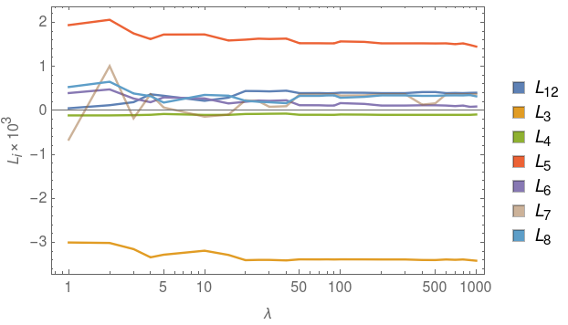
In Fig. 2 we show the value of and in Eq. (54) as a function of for the minimization of the Hadron Spectrum Collaboration -meson phase-shift data at MeV Wilson et al. 2015 together with decay constants from MILC Bazavov et al. 2010a. The LEC values obtained are given in Fig. 3. Clearly, for the LECs become stable while gets significantly reduced. One could also choose a higher value of , however, at the cost of increasing . Thus, we set the value of to .


.
There is an additional caveat that one should take into account; ChPT is built as an expansion in meson masses and, as such, the chiral series is only expected to converge for light pions. In order to study the convergence radius of ChPT we perform first individual fits of lattice data sets and discard pion mass results for which the fit does not pass the Pearson’s test at a % upper confidence limit. This restricts the lattice data sets to pion masses below around MeV. Results presented in the following sections beyond that pion mass are merely qualitative.
As a final remark, we want to point out that the uncertainties for our final global fit are evaluated using the bootstrap method and hence, the errors should be understood in terms of probability, i.e., our central values are given by the median of the distribution and the uncertainties are expressed in terms of the 68% and 95% confidence intervals.
III ChPT: Decay constant analysis
In this section, we attempt to perform a global fit of pseudoscalar meson masses and decay constants from Bruno et al. 2017; Blum et al. 2016; Bazavov et al. 2010a; Bazavov et al. 2010b; Aubin et al. 2008; Noaki et al. 2009; Aoki et al. 2009. These data are simulated on the chiral trajectories Blum et al. 2016; Bazavov et al. 2010b; Aubin et al. 2008; Aoki et al. 2009, Bazavov et al. 2010a, Noaki et al. 2009 and Bruno et al. 2017. The free parameters are the LECs , with , which appear in Eqs. (8)-(14), as well as the variables, and , which fix the chiral trajectories, and , respectively, according to Eqs. (47) and (48).
A few aspects need to be considered before. First, the role of the renormalization scheme used in the lattice simulations to fix quark masses. Here, we do not adjust quark masses values but pseudoscalar meson masses, which, in principle, should be independent of the renormalization scheme. Still, we checked if the pseudoscalar meson masses in the lattice data sets with different renormalization schemes are compatible. For example, we notice that UKQCD Collaboration uses the MS scheme at GeV Blum et al. 2016, while the MILC Collaboration uses the same scheme at GeV Bazavov et al. 2010a; Bazavov et al. 2010b; Aubin et al. 2008. When we compare both sets of data, we do not observe any substantial inconsistency, but instead, their values do agree quite well.
Second, other important issue is the size of the pion masses used in the simulations. We observe that in general the JL/TWQCD Noaki et al. 2009 and PACS-CS Collaborations Aoki et al. 2009 have larger pion and kaon masses. For instance, the JL/TWQCD pion and kaon masses are larger than and 600 MeV, respectively. These values might be too large for the perturbative ChPT expansion and indeed we are not able to fit these data sets in combination with MILC and UKQCD data. Thus, in this fit we only include data from Bruno et al. 2017; Blum et al. 2016; Bazavov et al. 2010a; Bazavov et al. 2010b; Aubin et al. 2008. The JL/TWQCD and PACS-CS data are studied in separated analysis in the next section.
Third, we should discuss possible finite volume and lattice spacing effects. In Bruno et al. 2017; Blum et al. 2016; Bazavov et al. 2010a; Bazavov et al. 2010b; Aubin et al. 2008, the dependence of the decay constant determinations with the lattice spacing was studied carefully and the results were extrapolated to the continuum. These extrapolated data are the input of the fit we show here. Another difficulty that we find to study data from Aoki et al. 2009 (PACS-CS) is the following. In Aoki et al. 2009, the chiral trajectory is set in such a way that the physical point of the strange quark is determined and later fixed onto the chiral trajectory of the simulation. Thus, the dependence on in principle should agree with that from MILC Bazavov et al. 2010a; Bazavov et al. 2010b; Aubin et al. 2008 and UKQCD Blum et al. 2016, since these simulations are also performed at the physical strange-quark mass. However, we found substantial discrepancies in the behavior of the chiral trajectory in Aoki et al. 2009 with those from MILC and UKQCD. These inconsistencies may be due to finite volume and discretization effects, which can be partly absorbed by the free parameters. The result from analyzing PACS-CS data, pseudoscalar meson masses and decay constants Aoki et al. 2009 together with -meson phase-shift data Feng et al. 2015, is shown in the next section.
Lastly, it is also pertinent to discuss the relevance of the scale setting. Different lattice collaborations use different methods to set the scale. While all of them should agree at the physical point, i.e., for physical quark masses at zero lattice spacing, different schemes might approach this point with different slopes. It implies that, for unphysical pion masses, lattice observables might be scale dependent quantities. Thus, from a rigorous point of view, one should only compare among lattice results using the same scale setting procedure, or at least, include this dependence as an additional uncertainty. Unfortunately, on one side, there is not enough lattice data from the same collaboration to study the dependence of the meson mass with the scale setting. On the other side, an extension of the IAM considering this effect is not available yet. In our particle case, the ensembles in Bruno et al. 2017 (see Table II of Bruno et al. 2017 for the pseudoscalar meson mass and decay constants of the CLS collaboration) consider two different scale setting methods, called here scale settings A and B. In the first one, scale setting A, the lattice spacing is determined by fixing the chiral extrapolations of and to the physical point. The second one, scale setting B, uses the Wilson flow () to set the scale by assuming that, for all different ensembles, the data over the trajectory intersects the symmetric line at , with . This method requires small corrections in the quark masses from the ones used in the simulations Bruno et al. 2017, which translates into small shifts for the pseudoscalar masses and decay constants. Nevertheless, the CLS -meson phase-shift data in Andersen et al. 2019 for the scale setting B were not shifted accordingly, and hence, these corrections could lead to a conflict among the CLS decay constant and phase shift data. Then, we take here the no-shifted values, first rows of Table II in Bruno et al. 2017. For each ensemble , these two scale settings lead to different lattice spacing values . Namely, fm for scale setting A and , fm for B Bruno et al. 2017. Nevertheless, we find that scale setting B produces systematically smaller values of than A for the same pion masses. For instance, we see a difference of around MeV in for pion masses of around MeV between the two scale settings. This difference is not small, since changes of MeV in imply variations on of around MeV in these data. Because of these discrepancies, we are only able to find an optimal when data with scale setting A are included. Notice that this is the method that fixes the scale using the and physical quantities.77 7 However, we show in section IV.2 that phase-shift lattice data in this scale setting cannot be reproduced globally. The reason is that the data for the ensembles N200 & N401 produce lower -meson masses than the predictions in the IAM. This problem is tackled in section V. In section IV.2 we analyze the decay constant data in combination with -meson phase-shift data for both scale settings and discuss the main differences.
| Fit I () | LEC |
|---|---|
| Fit I | |
|---|---|
In conclusion, it is only possible to do a combined fit of data from Bruno et al. 2017 (scale setting A) and Blum et al. 2016; Bazavov et al. 2010a; Bazavov et al. 2010b; Aubin et al. 2008.88 8 This fit passes the Pearson’s test. In Tables 1 and 2, the values of the fitting parameters obtained from this analysis are presented. This result is called Fit I. We notice that the LECs in this fit are not very sensitive to small variations of the and parameters, being thus quite stable. Furthermore, they are in line with the compilation of the FLAG Review Aoki et al. 2019, which only includes results for data. However, note that we are obtaining much smaller LEC errors compared to the FLAG average. Notice also that since these data include variations of the strange-quark mass, one is able to fix well the strange-quark mass dependence of the pseudoscalar decay constants for the pion masses studied.
The various chiral trajectories studied are shown in Fig. 4 (top-left panel), where one can see that the kaon mass squared data for the trajectory Bruno et al. 2017 differ considerably from the ones Blum et al. 2016; Bazavov et al. 2010a; Bazavov et al. 2010b; Aubin et al. 2008. In addition, two of the ensembles simulated in Bruno et al. 2017, the ones with and , lead to very similar curves and hence to similar values of in Table 2. Furthermore, the UKQCD Blum et al. 2016, MILC Bazavov et al. 2010a; Bazavov et al. 2010b and Laiho Aubin et al. 2008 lattice data are in very good agreement. Indeed, ChPT is able to reproduce well the data on these two different trajectories.
The ratios , and are also depicted in Fig. 4. For the ratio , it is worth noting that all data, independently of the chiral trajectory, lie almost on the same curve. This suggests that the ratio is indeed quite independent on . We discuss this further in Sect. V. In fact, all lattice data for this ratio fall into the gray error band plotted, which is just an extrapolation of the percentage error of this ratio at the physical point determined by MILC Bazavov et al. 2010b. For this collaboration only , and data are provided, which are shown with dashed black lines. The trajectory from Bazavov et al. 2010a is denoted by a solid gray line. The data of Laiho Aubin et al. 2008 is represented by dashed-orange lines. UKQCD data are denoted by black squares, while CLS data Bruno et al. 2017 are given by dark-green squares (), blue circles () and yellow pentagons (). Note that the UKQCD Collaboration and Laiho data sets provide very similar values of . In addition, we include in Fig. 4 the chiral prediction for the SU(3) trajectory. Both, and trajectories, lead to a substantial reduction of the ratios and . For pion masses larger than MeV, the ChPT prediction begins to differ from the data, which suggests the breakdown of the chiral series.
 |
 |
 |
 |
 |
 |
IV IAM: Rho phase shifts analyses
IV.1 Chiral trajectories
In this section we analyze the -meson phase-shift data from Dudek et al. 2013; Wilson et al. 2015; Bulava et al. 2016; Feng et al. 2015; Alexandrou et al. 2017 and pseudoscalar meson masses and decay constants from Blum et al. 2016; Bazavov et al. 2010a; Bazavov et al. 2010b; Aubin et al. 2008; Noaki et al. 2009. All these data are taken from simulations over chiral trajectories where the strange-quark mass is kept fixed to the physical value, , except for the JL/TWQCD, where Noaki et al. 2009. In fact, the pion and kaon masses used in the simulations of Noaki et al. 2009 are larger than in the other simulations. This simulation is studied independently and discussed at the end on in this section.
First of all, we perform individual fits to the pseudoscalar masses and decay constant ratios from UKQCD Blum et al. 2016, MILC Bazavov et al. 2010a; Bazavov et al. 2010b and Laiho Aubin et al. 2008 together with the -meson phase shift data from the HadSpec Collaboration Dudek et al. 2013; Wilson et al. 2015 corresponding to MeV. The LECs obtained in these fits are shown in the second, third and fourth columns of Table 3, respectively. Although some small differences among the individual fits are observed for and , they provide in general compatible LEC values within uncertainties. Thus, we conduct a simultaneous analysis of the UKQCD, MILC and Laiho decay constants and HadSpec phase shifts, which is denoted as MUL+HS in the fifth column of Table 3. As expected, the fit provides a good description of all data with consistent LECs.
Finally, we include the phase-shift results from Bulava et al. 2016 (JB) at MeV. This is denoted as Fit II in the sixth column of Table 3. Notice that this fit encompasses a large bunch of data on (). The LECs obtained in these fits are very similar to the previous ones suggesting consistency among the different data sets. Results for phase shifts together with the fitted lattice data are plotted in Fig. 6. As shown in Fig. 6 (left, top), the extrapolation of Fit II results to the physical point (light-blue solid line) is very close to experimental data, depicted as light-blue squares Protopopescu et al. 1973 and orange circles Estabrooks and Martin 1974.
Regarding decay constant ratios and pseudoscalar meson masses, results from Fit II are very similar to those obtained in Sect. III over trajectories, and are shown in Fig. 5.
 |
 |
 |
 |
 |
 |
 |
 |
 |
 |
Unfortunately, we could not obtain additional consistency with the lattice data from Feng et al. 2015; Alexandrou et al. 2017; Noaki et al. 2009. Thus, in the following, we analyze the remaining lattice results separately. The simulation of Alexandrou et al. 2017 (CA) for -meson phase-shift data does not include decay constant determinations, thus, we analyze this data with the UKQCD meson and decay constant values. If other decay constant data are used instead, as for example, those from MILC, the results are very similar. The resulting LECs, given in the second column of Table 4, are, in general, compatible with the values from Fit II, but we find slightly different values for and , and larger discrepancies for . These differences have a large impact on the phase-shift values. As shown in the right-top panel in Fig. 6, the extrapolation to the physical point provides results incompatible with experimental data.
Concerning the JL/TWQCD collaboration decay constant data Noaki et al. 2009, we only find good partial fits if we include the three and two lightest pion mass data points for the trajectories and , respectively. This can be due to the breakdown of the ChPT expansion for such large values. Since in these simulations decay constant determinations are provided but not phase shifts, we analyze them together with the Hadron Spectrum Collaboration (HS) -meson phase shift results at MeV. The only purpose of this fit is to show the qualitative behavior of the pseudoscalar meson mass and decay constant ratios over trajectories with larger values than the physical one. The corresponding LECs obtained in the fit are given in the third column in Table 4. A comparison with the result from Fit II in Table 3 shows up sizable discrepancies between both fits, which might be due to inconsistencies of the JL/TWQCD data with data included in Fit II apart from the breaking of the chiral series. These phase shift results are also plotted in the top-left panel of Fig. 6 in dashed lines. Nevertheless, the extrapolation to the physical point of this fit turns out to be also very close to the experimental data.
For the PACS-CS collaboration, both -meson phase shift Feng et al. 2015 and decay constant Aoki et al. 2009 data are available and analyzed together. The LECs are given in the fourth column of Table 4, and also the ’s, , differ considerably from the Fit II values. As explained in Sect. III these data have larger kaon masses for the same trajectory than data in Fit II. This can be due to sizable finite volume effects in these simulations. As a consequence, these data are in disagreement with the data included in Fit II. In this case, the extrapolation to the physical point, depicted in the bottom-right panel of Fig. 6, fails substantially to describe the experimental data.
Let us note that these -meson phase-shift data were analyzed before in Hu et al. 2017 using the UChPT model in Oller et al. 1999. Even though this model neglects the LHC contribution, which now is taken into account, we obtain here similar results to the ones of Hu et al. 2017.
The chiral trajectories and decay constant ratios for these fits are shown in Fig. 5. We find that the pseudoscalar meson mass data on trajectories fit very well into a linear formula with slope , depicted in dotted lines. This behavior is qualitatively similar to the leading order ChPT prediction. For the ratios of decay constants we find similarities with the results of Fit I over the trajectory . The ratios and in other trajectories as a function of the pion mass are parallel to the ones over and take higher values. For the ratio, only the JL/TWQCD and PACS-CS data are just a bit out of the error band.
 |
 |
 |
 |
Finally, the pole position on the second Riemann sheet obtained in the different fits are given in Table 5. While the values obtained in Fit II and in the JL/TWQCD & HS fits are compatible with the most precise theoretical prediction Garcia-Martin et al. 2011b, the results obtained for UKQCD & CA and PACS-CS provide smaller and larger values, respectively. In order to write down results that can be compared to the BW values provided in lattice articles, we perform a refit of the IAM solution to the BW formula in Eq. (64). As we show in Fig. 42 in the Appendix VII.2, the data is also well described by a Breit-Wigner (BW) parameterization. The BW mass, coupling and width, normalized to the pion mass, are shown in Table 5, where we also provide the result for the extrapolation to the physical point.
| LEC | MILC+HS | UKQCD+HS | Laiho+HS | MUL+HS | Fit II |
|---|---|---|---|---|---|
| LEC | UKQCD+CA | JL/TWQCD+HS | PACS-CS |
|---|---|---|---|
| (MeV) | ||||||
|---|---|---|---|---|---|---|
| Fit II | ||||||
| UKQCD&CA | ||||||
| TW/JLQCD&HS | ||||||
| PACS-CS | ||||||
IV.2 Chiral trajectories
In this section we show the outcome of the analysis of -meson phase-shift Andersen et al. 2019 and decay constant Bruno et al. 2017 data of the CLS Collaboration over trajectories where , see Tables II of Bruno et al. 2017 and 6-11 of Andersen et al. 2019. Thus, in these trajectories the kaon becomes lighter as the pion mass increases. Two different scale setting methods were considered in Bruno et al. 2017. These two methods lead to differences of around MeV in , MeV in , and MeV for and . These differences entail several difficulties. As discussed in section III, we could only find an optimal solution to the minimization problem of Fit I, that also includes data, when scale setting A was taken for the pseudoscalar meson masses and decay constants over the trajectories. When the scale setting B was considered instead, the global minimum was found to be around twice larger than with the scale setting A. On the contrary, we observe that, when using scale setting A, the dependence of -phase shift data with the pion mass of Andersen et al. 2019 cannot be described well within the IAM for all ensembles. While the ensembles D101, J303 and D200 are well described, the ensemble N200 (or N401) cannot be reproduced. This is because the IAM predicts higher values of the meson mass for the pion mass used in this ensemble, see Fig. 7 (Fit IIIA). Interestingly, by using scale setting B, we find a solution describing all lattice data, i.e., pseudoscalar meson mass and decay constant ratios and -meson phase shift (excluding data). These phase-shift results are plotted in Fig. 8 (Fit IIIB).


Nevertheless, it is possible to perform fits of decay constant and -meson phase shift data for ensembles with the same gauge coupling Andersen et al. 2019. Namely, C101, D101 (), N401 (), N200, D200 () and J303 (). Several of these ensembles use the same pion mass but different volume or lattice spacing. On one side, the ensembles C101 and D101 are simulated with the largest lattice spacing but D101 uses a volume times bigger than C101. On the other side, the ensembles N200 and N401 were simulated in the smallest volume but N200 has a lattice spacing times smaller than N401. Finally, J303 has the biggest volume and smallest lattice spacing.99 9 The volumes of the C101 and D101 ensembles are and respectively, both with a lattice spacing fm (scale setting B). The lattice spacings for N401 and N200 are fm and fm, respectively, and both have the same volume . J303 has fm and is simulated in a volume . The volume and lattice spacing used for D200 are and fm, respectively. In this way, possible differences between individual fits in these pairs might highlight finite volume and lattice spacing effects. The resulting LECs are shown in Tables 6 and 7 for the A and B , respectively. The ensembles C101 and D101 are fitted separately in order to study the finite volume effect. Overall, the values of the LECs and are approximately stable, but we find large differences for the others.
We also attempt to perform combined fits including most ensembles for different in order to check whether these effects can be absorbed in the LECs. Since the D101 and N200 ensembles supersede the C101 and N401 ones, accordingly, we only include the ensembles D101, N200, D200 and J303. These fits are denoted as Fit III A and III B for the A and B scale settings, respectively, and they also include the corresponding pseudoscalar meson mass and decay constant ratio data. The LECs obtained are given in the last columns of Tables 6 and 7.
In general, the LECs of Fit IIIA agree better with those obtained for the trajectories. The chiral trajectories and decay constant ratios of these fits are depicted in Fig. 5 (right), where we also show the result of the fits for comparison (left panel). Results for the fits IIIA and B are plotted in like blue-solid and green-double-dot-dash lines, respectively. The kaon mass dependence on the pion mass for the trajectories also fit well into straight lines, , but now with a slope close to instead of , as we found for the ones. In this way, the IAM is able to reproduce very well the trajectories, which appear as three close decreasing curves intersecting the symmetric line, . At pion masses of MeV, the kaon mass is around MeV lower than for the trajectory.
The ratios of decay constants are also well reproduced. For the scale setting A, the ratio agrees well with the data, emphasizing that this ratio is almost independent of . In the case of scale setting B, it falls a bit out of the error band, depicted in a light-brown color. Note that this behavior is different from the trajectory (MILC, dotted-gray), which lies inside the error band and does not show any substantial difference with the curve. This suggests that there could be small dependencies with the strange-quark mass. We comment more on this issue in the next section.
Results for -phase shifts are provided in Figs. 7 and 8. As commented before, except for the ensemble N200 in scale setting A, all the other phase shifts can be described qualitatively well in these fits. In Figs. 9 and 10 we show the -meson phase shifts obtained for the different gauge coupling fits. The IAM allows one to describe the -meson phase-shift data in trajectories for every ensemble. Nevertheless, note that one can not observe a trend of the overall data indicating that the -meson mass1010 10 Understood as the energy for which the phase shift is . increases monotonically with the pion mass. Namely, for scale setting A, the N200 and N401 ensembles give rise to a lighter -meson mass than the ensembles D101 and C101 even when they are simulated with heavier pion masses. In addition, the -meson mass takes about the same value for the J303 and D101 ensembles, although the pion mass used in J303 is around MeV larger. Similar results have been observed in a recent two-loop SU(2) IAM analysis of the same CLS data Niehus et al. 2020.
At low energies, phase shifts decrease as the pion mass grows, as expected from the -wave centrifugal barrier and the chiral expansion. For scale setting B one observes that the trend of the -meson mass dependence on the pion mass is flatter. Noticeably, the -meson becomes lighter for pion masses around MeV in both scale settings. In both cases, systematic effects due to a finite volume and lattice spacing are reflected in around MeV difference in the -meson mass between the C101 and D101 and MeV between the N200 and N401 ensembles, respectively.
The corresponding pole positions and couplings for both scale setting are given in Table 8. In addition, given the large discrepancies observed between the scale settings we perform a new fit with their average for each gauge coupling , denoted as Fit C in Table 8. For comparison, the result of the global fit including both data on and Tr trajectories, discussed in the next section (Fit IV) is also shown. The values are normalized to the pion mass, so that the dependence of the ratio with the pion mass and scale setting used is visible. Overall, we see that the results for different lattice spacings are quite similar. For the ensemble J303 the dependence on the scale setting considered is negligible, while for other ensembles it produces shifts of less than 1% for the normalized mass and less than 5% for the couplings. Regarding finite volume and lattice effects, the systematic differences between C101 and D101 are of around 1% in the normalized mass, and 1.5% between the N200 and N401, while these are of less than 2% in the couplings in both cases. Finally, the comparison between the individual fit solutions obtained using A and B scale settings is given in Fig. 11, where it can be seen that the differences produced in phase shifts as a function of are in general reasonably small, and negligible for the J303 ensemble. The largest difference is coming from the size of the lattice spacing used in the simulation, i.e., the difference observed between the N200 and N401 ensembles.
Finally, we can compare the result of Fit C in Table 8 with the result of Fit IV which includes also data. There are small differences between these two fits of less than 3% in the normalized -meson mass and less than 6% in the couplings. We discuss this further below.
| LEC | Fit IIIA | |||||
| Ensemble: | C101 | D101 | N401 | N200, D200 | J303 | D200, N200 |
| J303, D101 | ||||||
| LEC | Fit IIIB | |||||
| Ensemble: | C101 | D101 | N401 | N200, D200 | J303 | D200, N200 |
| J303, D101 | ||||||


| (MeV) | ||||||
| D200 | A | 209 | ||||
| B | 200 | |||||
| C | 204 | |||||
| IV | 204 | |||||
| C101 | A | 244 | ||||
| B | 223 | |||||
| C | 233 | |||||
| D101 | A | 244 | ||||
| B | 223 | |||||
| C | 233 | |||||
| IV | 233 | |||||
| J303 | A | 267 | ||||
| B | 258 | |||||
| C | 263 | |||||
| IV | 263 | |||||
| N200 | A | 297 | ||||
| B | 283 | |||||
| C | 290 | |||||
| IV | 290 | |||||
| N401 | A | 297 | ||||
| B | 283 | |||||
| C | 290 | |||||
| IV | 290 |
V Global fit over and trajectories: Fit IV
In this section we perform a simultaneous analysis of lattice data over both and trajectories. This final study will be denoted as Fit IV and it analyzes lattice -meson phase shift data in of Dudek et al. 2013; Wilson et al. 2015; Bulava et al. 2016; Andersen et al. 2019 in combination with pseudoscalar meson masses and decay constants from Bruno et al. 2017; Blum et al. 2016; Bazavov et al. 2010a; Bazavov et al. 2010b; Aubin et al. 2008. Thus, this analysis takes into account all data included in the fits II and III of Sects. IV.1 and IV.2.
As discussed in Sects. III and IV.2, we were not able to find a solution with the IAM describing data on trajectories using either of the scale settings in Andersen et al. 2019; Bruno et al. 2017 in combination with data over . Hence, in order to attempt a global fit some remarks are necessary. First of all, the ensemble C101 of Andersen et al. 2019 will be discarded since the simulation for the ensemble D101 is performed in a larger volume. Note that even when the N401 ensemble has larger lattice spacing than the N200, the former has more data points and its uncertainties are smaller, therefore, we include both ensembles in the present analysis. Secondly, it is important to highlight that, according to Tables 5 and 8, the CLS result for the ratio of the D101 ensemble is very close to the one from the HadSpec (HS) collaboration at MeV, Fit II; the difference is only of around 2%. This fact points out that the pion masses used in these simulations should also be very similar. Nevertheless, only the average between the scale setting A and B has a similar pion mass ( MeV). This facts motivates us to consider that the average between both scale settings provides a reasonable estimate to be used in order to perform a global fit of data. Hence, we perform a bootstrap of the lattice spacing for the ensembles assuming that for every , it is normally distributed around the average of scale setting A and B and the standard deviation being half the difference between them. Not only the lattice spacings, ’s, but also decay constant ratios and energy levels (normalized respect to the pion mass) for each ensemble are generated from a normal distribution accordingly to their lattice data errors. Regarding the lattice energy levels, the resampling is performed assuming a multivariate normal distribution with the original covariance matrix.1111 11 Phase-shift data are then obtained from a first order Taylor expansion around the lattice data energies.
Remarkably, following this strategy we could reproduce decay constant and phase-shift data simultaneously on both trajectories. The resampling is performed 300 times and the error is evaluated from that sample. This number of fits turns out to be enough, since the average, median and fit solution (taking the average of the lattice spacing) are indeed very close to each other. Namely, they produce differences in the -meson mass of less than MeV. Since we are interested on interpreting the results in terms of probability and confidence intervals, our central results are represented by the median or first quartile and the uncertainties will be described by the 68% and 95% confidence intervals (CI), which are represented as darker and lighter error bands, respectively.
Finally, let us remind that here we are only considering the systematic error associated to the scale setting for the CLS data Andersen et al. 2019; Bulava et al. 2016, which has much larger effects (as discussed in Sect. III) than the one observed in the HS data Dudek et al. 2013; Wilson et al. 2015; Bolton et al. 2016. The latter was investigated in Hu et al. 2017, where the two different lattice spacings from Bolton et al. 2016 were considered, leading to a difference in the mass of less than , which is neglected here (see Table II of Hu et al. 2017).


 |
 |
 |
V.1 Results for meson masses and decay constants
In Figs. 12, 13 and 14, the chiral trajectories and pseudoscalar meson mass and decay constant ratios studied are plotted. The lattice data fitted correspond to the extrapolation to the continuum limit with finite volume effects corrected. In more detail, for the trajectory we include the UKQCD Blum et al. 2016 (purple diamonds), MILC Bazavov et al. 2010a; Bazavov et al. 2010b (black dashed curves with light-brown error bands1212 12 The data was sent to us by C. Bernard and the error band is extrapolated from the physical point as suggested by him.) and Laiho Aubin et al. 2008 (orange dashed curves and error bands) lattice data. For other trajectories there is not much data except for the ratio extracted by MILC Bazavov et al. 2010a for (gray dotted line). The data from the CLS Collaboration are given for the different lattice gauge couplings (green squares), (red circles), (blue triangles) and (yellow pentagons). The error in the pion mass (x-axis) corresponds to half the difference between the pion mass using the two A and B scale settings. Although in principle chiral trajectories for the several gauge couplings are different, in practice, we obtain very similar curves when the error in the lattice spacing is considered, which only start to separate more clearly when these cross the symmetric line. This is, we get and only a small difference for . In addition, we include in Figs. 12, 13 and 14 the IAM prediction for the trajectories , which are almost parallel to the one. Furthermore, in order to highlight the relevance of the strange-quark mass, we also include the prediction for the trajectories 1313 13 In this case, it is understood that . and . These three trajectories start at a small value of (), then, they cross the symmetric line and end up at the curve. All ratios , , and are reproduced well inside the % CI till MeV, when the ChPT predictions start to deviate. Therefore, the predictions for pion masses between MeV are merely qualitative.
The extrapolation to the physical point for the mass and decay constant ratios is given in Table 9. The central value represents the median, while the first upper and down indices show the limits of the 68% CI. The upper (down) limits of the 95% CI are obtained by summing the absolute values of the first and second upper (down) indices. These extrapolated ratios are compatible with the experimental values, which are inside our CI.
| Experiment [PDG] | |||
The values of the LECs and remaining fit parameters are given in Table 10, where errors also represent and CI. The quark condensate can be estimated for a given strange-quark mass from Table 10. For instance, taking MeV we obtain MeV, in close agreement with the MILC result Bazavov et al. 2009, MeV. Finally, the correlation matrix of the parameters is given in Eq. (77) in the Appendix VII.3.
| () | LECs |
|---|---|
| , | |
| Tr M() | |
| Tr M() | |
| Tr M() | |
Strange-quark dependence of the pion mass and decay constant
From Fig. 13 one sees that the ratio does not depend much on . However, this does not necessarily mean that is independent of the strange-quark mass. In fact, both and depend on . This dependence is shown explicitly in Figs. 15 and 16. In Fig. 15, the squared leading order mass, , is depicted as a function of the pion mass for different strange-quark masses. Indeed, one can see that kept constant does not imply that the pion mass is constant as well. In fact, our analysis at one-loop level predicts that the pion mass grows with for a constant value of ; while for one obtains (see the red line in Fig. 12) and (notice the almost quadratic behavior of the red curve in Fig. 15), consistently with the leading order ChPT prediction, effects coming from the kaon and eta particles in become more relevant as increases. Although this effect is invisible for very light pion masses and small for physical pion masses (for a constant value of , the difference between the physical pion mass and the value at in Fig. 15 is around .), it becomes larger for heavy pions. On the contrary, in Fig. 16, where the dependence of on for different strange-quark masses is shown, one sees that this dependence is more noticeable for light pion masses and smaller for heavier pion masses, when the uncertainties for increase. At the physical point, one indeed finds a difference of MeV in between its value at and . This is intrinsically connected with the contribution of the terms which involve kaons and etas in Eqs. (8) and (12),
| (56) |
with
| (57) | |||
| (58) |
which are
| (59) | ||||
| (60) |
These terms, which involve kaon and eta meson loops (tadpoles) and kaon mass contact terms, called from now on, contribute slightly for , around MeV in the value, but they account for about MeV at . Later, we show that this relatively small variation in is translated into a visible difference in the mass.
Beyond that, one might wonder what would happen in a world where kaons and etas are not present. In order to answer that question, we could explicitly set to zero the contribution in Eqs. (8) and (12), and define and in Eqs. (57) and (58) as the pion mass and decay constant in this world. In such a way, one obtains a dependence of the new pion decay constant, , with the pion mass, as the orange-dashed line in Fig. 16. Effectively, this limit is equivalent to set the coupling of pions to kaons and etas to zero, which can be achieved when, first, in Eqs. (13) and (14) are sent to infinity,1414 14 Note that it can only achieved if one breaks the SU(3) symmetry in the partially conserved axial current (PCAC), i.e., one has to differentiate between the pion and the kaon and eta decay constants in the chiral limit. See explanation in Sect. VII.1. and, second, when are set to zero. This is discussed in Sect. VII.1. Furthermore, note that this is different from the so-called SU(2) formalism (corresponding to take the limit ), where the effect of pions interacting with kaons and etas is absorbed in the SU(2) LECs, the constant and , which are fixed, together with , to get observables in the physical world with more than two flavors.


When , reduces its value around MeV at the physical point, while it approaches the value of the chiral trajectories and as the pion mass decreases, reaching in the chiral limit. These interacting terms involving kaons and etas have a similar effect to the one caused by a change in for light pion masses. In fact, varying from zero rises the contribution of these terms, increasing the value of .
We can also compare the ratios obtained here with the ones of the simulation of Guo et al. 2016. For the pion masses used in that simulation, and MeV, the ratios are and ,1515 15 Where we have divided from Guo et al. 2016 by a factor according to the normalization of used here. for the light and heavy pion mass, respectively. Looking at Figs. 12, 13 and 14, we see that the deviations from the mean values in Fit IV at the trajectory are of less than for the light pion mass, and around for the heavy pion mass. These relative differences are small and the ratios in Table III of Guo et al. 2016 are compatible with our error bands. This indicates that the setup of the simulation of Guo et al. 2016 is in line with the result of this analysis for the chiral trajectory. Thus, possible deviations in the -meson parameters with the ones obtained here might be caused by a different reason. Notice also that the method used to determine these ratios in Guo et al. 2016 is to take to the physical point in a strange-quark quenched approximation. As a consequence, the values of obtained are consistent with the ones from Fit IV at and its extrapolation to the physical value. However, since the real world has more than two flavors, that approach misses the dependence of as discussed before.
V.2 Results for the -meson phase shift and pole parameters
Phase shift lattice data and solutions from Fit IV at the corresponding pion masses are depicted in Figs. 17, 18, and 19, where one can see that lattice data are very well described also inside the % CI. The only exceptions are few data points from the CLS data for the N200 and N401 ensembles (right-bottom panel in Fig. 18), which lie outside the error band and are also far from the bulk of data. Beyond that, most of data for these ensembles are inside of the 95% CI error bands. This is, the N200 and N401 ensembles are compatible within uncertainties, as concluded also in Andersen et al. 2019. Note that the error bands are larger for the data since they include the variation of the lattice spacing between A and B scale settings.
The extrapolation to the physical point in comparison with experimental data is plotted in Fig. 20, where one can see that it indeed provides an excellent description of the experiment. In Fig. 21, the CLS D101 ensemble and HS data for MeV are plotted together. We can see that indeed both results are compatible.
The phase-shift solution for the pion mass used in the D101 ensemble (dark green) is shown in comparison with the result from an individual fit of the C101 data (light green) in Fig. 22.1616 16 The average between the lattice spacings in scale settings A and B is taken in this individual fit of the C101 data in order to compare with the solution from Fit IV. Note that even when the C101 ensemble was not included in the global Fit IV, both solutions, and the bulk of data itself, lie well inside the 95% CI. The difference between both fits for the energy at which the phase shift crosses () is of around . This indicates that the deviations due to the volume size are not large.
 |
 |
 |
 |
 |
 |


To show the trend of the data, the mean solution of Fit IV together with the lattice data are represented in Fig. 23.1717 17 This correspond to using the averaged lattice spacing values as the data plotted in the figure. As can be seen, these data are now well described. Phase shift data corresponding to higher pion masses fall more to the right and the -meson mass increases monotonically with the pion mass.

The dependence of the -meson mass1818 18 Defined as the value of the energy for which . with the pion mass is depicted in Figs. 24 and 25 for the and trajectories, respectively, where we also show the values of the -meson mass given in the corresponding lattice papers.1919 19 For the trajectories, the error due to the use of scale settings A and B is also depicted. The ratios are also represented in the right panels. For clearness, we present again the lattice data and the resulting curves separately in Fig. 26. In both trajectories increases with . Furthermore, for the trajectories and , we find almost identical results till pion masses of around MeV, when these start to separate. The reason for this behavior is well understood. On one side, the meson becomes a bound state at pion masses around MeV in the trajectory (above this value, the threshold is plotted in Figs. 24 and 26 (left) instead). On the other side, it starts to decay into in the trajectory when the -meson pole crosses this threshold and the kaon gets lighter than the pion. Indeed, it becomes a pole in the IV Riemann sheet as defined in Eqs. (43) and (). Conversely, other trajectories tend to be flatter than the ones. This is actually in line with the trend of lattice data.
It is relevant to note that close to the physical point we do not observe any relevant change in the -meson mass. This suggests that the -meson properties are quite stable against small variations of the strangeness around the physical point, however, its coupling to the channel is still large, around of its coupling to . 2020 20 This can be seen in Figs. 34 and 35, as discussed later in this section. . Nevertheless, for values below , the -meson mass starts decreasing considerably reaching a value inside the interval MeV for . This behavior is even more clear in the trajectories where the mass of the quark (or pion) is kept fixed and only varies. Since the meson starts to decay into for lighter strange quarks, the effect in the real part of the pole, see Fig. 29, becomes significant.
This behavior of the -meson mass is also visible in the corresponding plots (right panel of Figs. 24 and 25), where the errors in the y-axis are reduced. These plots also show that the error due to the lattice spacing (or scaling setting used) is smaller than the reduction of the -meson mass around the limit. The behavior of the -meson mass and width respect to the kaon mass is depicted in Fig. 29 for the and trajectories. When decreases, both mass and width decrease, as commented before. In Figs. 27 and 28, the continuation of the ratios for smaller pion masses are also depicted. This difference with respect to the physical point is more abrupt as the quark masses get smaller. The symmetric line is also plotted in dot-dashed lines.
 |
 |
 |
 |
 |
 |


 |
 |
In Figs. 30, 31, 32 and 33 we provide the real and imaginary parts of -meson pole position in a 3D plot respect both, the pion and kaon mass. To render some references, we also give in Table 11 the pole positions at for pion masses near the chiral limit, physical point and when the gets bound ( MeV in the last two trajectories).
| MeV | |||
| MeV | |||
| MeV | |||
| MeV | |||
| MeV | |||
| MeV |
Let us start analyzing the -meson behavior in the trajectory. See Figs. 30, 31. In this case, we obtain a -meson pole position MeV near the chiral limit, while at the physical pion mass we get MeV, see Table 11, consistently with previous analyses Ruiz de Elvira et al. 2017. Nevertheless, as increases, the -meson mass moves slower than the threshold, so that, eventually, the meson becomes a bound state with a mass around MeV for a pion mass of around 450 MeV. Note that, in the case of the trajectory, the -meson pole is always below the threshold for the pion masses analyzed here. We do not start to appreciate significant changes in the behavior of the -meson mass till the strange-quark mass is reduced in half its physical value. For instance, for , we still get a pole at MeV in the chiral limit, which transforms into a bound state with a mass of MeV also for pion masses of around MeV. For lighter strange-quark mass trajectories relevant changes are observed. Both, -meson mass and width, decrease consistently, so that we obtain MeV for in the chiral limit. Furthermore, for , both the and thresholds get closer to each other as increases, in such a way the kaon becomes lighter at a given point. In this regime, the meson becomes a pole in the fourth Riemann sheet2121 21 The Riemann sheet that is reached when only the cut is crossed continuously from the first Riemann sheet. when its mass gets below the threshold. In this case, the -meson decays only into and its width starts increasing again until it gets a maximum, after which the eventually becomes a bound state as increases.
This behavior is even more noticeable for the trajectories, depicted in Figs. 32 and 33. In this case, the strange-quark mass decreases as grows reaching the symmetric line for pion masses of around 450 MeV. Once the symmetric line is crossed, the channels opens below the two-pion threshold and the meson becomes again a pole on the fourth Riemann sheet. Nevertheless, the kaon mass in this trajectory decreases till it ends up in the line (red-solid curve). Hence, the -meson mass (width) starts decreasing (increasing) at a given point (when the kaon gets lighter than the pion after crossing the symmetric line) till ending at the zero strangeness line. This behavior suggests that strangeness plays an important role in the meson near the SU(3) flavor limit. This can also be inferred from the increase of its coupling to , as discussed below.2222 22 At the symmetric line, the coupling to grows of its value at for physical pions.
The pion mass dependence of the -meson couplings to the and channels, and as defined in Eq. (45), are shown in Figs. 34 and 35 for the and trajectories, respectively. On one hand, varies smoothly with before the the -meson transition into a bound state, decreasing as it approaches the threshold and increasing with . Once the meson becomes bound, its coupling rises sharply till MeV. Overall, it takes values for the range of pion masses studied. On the other hand, and contrary to the behavior, decreases significantly with the mass of the strange quark. In addition, while the pion-mass dependence of flattens for lighter strange quarks, it becomes larger as reaches the physical value. All in all, it takes values within the range to .
More information can be extracted when the ratio of both couplings is depicted, we refer to Fig. 36. Remarkably, for those regions where one observes the ratio . On the contrary, when . In the symmetric line we obtain exactly . This is not a coincidence. In the SU(3) limit, the decomposition of a , state of the antisymmetric octet representation into two-Goldstone–Boson states with well defined isospin reads
| (61) |
where, stands for the hypercharge and is the isospin. Thus, taking into account the kaon degeneracy due to strangeness, the -meson coupling to pions should be a factor times larger than for kaons. Notably, the IAM analysis presented here reproduces exactly the SU(3) limit prediction.
In Fig. 37, the ratio is depicted.2323 23 In this figure, means the real part of the pole position, , so that we are able to plot the ratio for a larger range of pion masses and after the transition. Since pole positions are slightly lower than the energy corresponding to , this ratio gives values lower in around , than if is taken. This ratio lies within the interval , i.e., close to , for the quark masses studied in this work, as predicted by the KSFR relation Riazuddin and Fayyazuddin 1966. Thus, we find that KSFR is qualitatively valid, being more accurate near the chiral limit, specially for the curves, and well applicable also around the physical point, with deviations from KSFR of less than 4%. The largest deviations (still smaller than 8%) are found for pion masses between and MeV.


 |
 |
 |
 |
 |
 |
 |
 |
To compare the LECs obtained in the different analyses done here with the Flag average Aoki et al. 2019, we depict them in Fig. 38, where we show the results from Fit I (pseudoscalar meson mass and decay constant ratios), Fit II, (analysis of data over the trajectories), Fit III, ( trajectories), and Fit IV (mean and standard deviation as a result of the study including both and trajectories) together with the Flag average (pink color). Indeed, we see that LECs from fits I and IV are very close, being also consistent with the FLAG average, which has larger errors. In general, fits I, II, IIIA and IV give closer results, while the LECs and , from the analyses of PACS-CS and JL/TWQCD data, strongly disagree with other analyses. Notice the precise values of the LECs provided by Fit IV.
 | ||
|---|---|---|
 |
 |
 |
 |
 |
 |
The role of strangeness on the -meson properties
As we did before when discussing , we can study the -meson properties in a world where there are no kaons or etas by setting to zero their corresponding interacting terms, i.e., contact mass terms and diagrams involving loops with kaons and etas in Fig. 1 and pions in the initial and final state, (what we called ). In practice, this means that we solve the one-loop IAM equation, see Eq. (34), taking the limits , and . We refer the reader to a more extended explanation in Sect. VII.1. Then, the pion mass and decay constant are given now by and in Eqs. (57) and (58). The result is shown in Fig. 39. Taking into account that we did not include data in our analysis but this result comes out as a prediction from our SU(3) IAM analysis, the agreement with the data from Aoki et al. 2007; Lang et al. 2011; Bali et al. 2016; Guo et al. 2016 is astonishing.
In fact, starting from a three-flavor formulation, the formalism should be in principle obtained when one decouples the strange-quark contribution by sending to infinity Gasser and Leutwyler 1985. In this case the effect of kaons and etas is encoded into the bare pion decay constant, , the constant , and in terms proportional to ( refer to the limit where , which can be absorbed in a redefinition of the LECs. Here, though, we are simply studying the world where there are no kaons or etas relying on the fact that their interaction with pions comes from terms where their masses and decay constants appear explicitly.
Lattice simulations typically use either Guo et al. 2016; Fritzsch et al. 2012 or the nucleon mass (via the QCD static potential) Gockeler et al. 2008; Feng et al. 2011; Lang et al. 2011; Bali et al. 2016 to fix the scale, which in general requires to perform a chiral extrapolation. Nevertheless, given the observed dependence of and on the strange quark, and the fact that is correlated with and the nucleon mass, these methods seems to neglect this dependence. In fact, the agreement between lattice simulations and the IAM prediction without kaons and etas on the -meson properties suggests that lattice simulations leave out the contributions coming from the strange quark, and hence, they describe a world where the strange-quark is missing.
In Fig. 40 we compare this result with Fit IV over the chiral trajectories and . Moreover, we also show the result of solving the one-channel IAM equation with , this is, keeping the terms in the channel. Remarkably, the one-channel IAM result for (orange line), (dashed-red), and the two-coupled channel solution over (dotted-red), provide very close results for the mass, which are also consistent with the lattice data. This is explained because the contribution of terms for light strange-quark masses is small. As explained before, these terms contribute in around MeV of the value when , and around MeV for at the physical pion mass, see Fig. 16. This reduction on the value of for smaller strange-quark masses reflects also in smaller -meson masses. Notice that in the trajectories, pions and kaons are acting effectively in the -meson mass as if only one flavor, the quark , is present.
It is also interesting to see what happens if one keeps the terms in and in the scattering amplitude when solving the one-channel IAM equation in the trajectory (dot-dashed blue). We see that this trajectory is consistent with the coupled-channel IAM solution for , telling that the effect of the off-diagonal elements in Eq. (II.3) is very small for physical strange-quark masses. Nevertheless, the coupled-channel effect becomes appreciable for lighter , as as one can see by comparing the difference between the dashed and continuous red lines. The small contribution of the off-diagonal elements at the physical point is in contradiction with the results in Guo et al. 2016; Hu et al. 2016, where the absence of these elements are found to be responsible for the dropping of the mass in the case. However, this is natural since in these works the same value of was used in the and predictions, and then, the effect of the kaon and eta contributions were absorbed in the off-diagonal elements. Indeed, we obtain here similar predictions for the meson mass in and simulations over than in Guo et al. 2016; Hu et al. 2016. Nonetheless, we have gone through a deeper analysis in this work; by studying the dependence of , we have obtained that regulates the contribution of the kaon and eta interacting terms and that the effect of these loops are absorbed in instead. Consistently with the predictions done in the works of Guo et al. 2016; Hu et al. 2016, we also obtain that the mass is reduced when these terms are omitted. In Guo et al. 2016, the pion decay constant was determined and these values were used to make predictions for the mass using the UChPT model in Oller et al. 1999 with two and three flavors. Nevertheless, the pseudoscalar meson decay constants in Guo et al. 2016 were determined following the method of Fritzsch et al. 2012 where the kaon is introduced later in the quenched approximation and is fixed to the physical point. This leads to extrapolated values of in simulations consistent with the experimental value, where more than two flavors do exist. However, by doing this, one is missing the dependence and the effect of the kaon and eta loops in the pion decay constant, that we have shown here. These missing effects can lead to discrepancies between observables in , such as the values of the mass and pion decay constant determinations. We have shown that a lower value of the mass than the physical one should be reflected also in lower values of . In summary, assuming that the pion decay constant is the same in the two and three flavor simulations totally misses the effect of the strange quark and loops containing kaon and eta particles in pion observables.


V.3 Comparison with new and lattice results
After our analysis was completed, several Erben et al. 2020; Fischer et al. 2020 and Werner et al. 2020 new simulations have been performed using the pion decay constant to fix the scale. The comparison of these results with our analysis for the -meson mass is depicted in Fig. 41. Looking at this figure it is clear that most data from Refs. Fischer et al. 2020; Erben et al. 2020 and Werner et al. 2020 follow a different trend than the data analyzed in this article and the data from previous simulations Aoki et al. 2007; Lang et al. 2011; Bali et al. 2016; Guo et al. 2016. Moreover, the new simulation in Fischer et al. 2020 includes results at the physical pion mass, which provide a -meson mass from a IAM analysis around MeV, i.e., much lower than all other predictions in two flavors. In order to try to identify possible sources of discrepancies, we have summarized in Table 12 the typical volumes and lattice spacings used in the simulations at different number of flavors. Comparing the data from Fig. 41 and Table 12, we would like to make some final remarks regarding the differences observed among simulations with different number of flavors:
- 1.
For MeV, the ETMC simulation Werner et al. 2020 obtains bigger values for the -meson mass than in the simulation of the same collaboration for MeV, even though the volume used in the simulation is bigger. This clearly points out that the dynamics involving the strange quark could be relevant in these simulations.
- 2.
The large discrepancy between the HS simulation Wilson et al. 2015 and the ETMC19 result Werner et al. 2020 at MeV, cannot be explained because of the different volume or lattice spacing used. Namely, the HS data are compatible with the CLS simulation around when the systematic error due to the lattice spacing is included ( % of the mass), even when CLS uses bigger volumes and smaller lattice spacing than HS. Similarly, these effects cannot explain the difference between the CLS simulation and the one at MeV. Then, these deviations between the and data can only be tight to the different methods employed by the collaborations in the simulations.
- 3.
The data for and simulations of the same ETMC collaboration show different trends of the -meson mass dependence with the pion mass. Remarkably, an extrapolation by the eye of the simulation would lead to a much larger value of the -meson mass than the simulation for physical pion mass of the data.
- 4.
The two simulations done at physical pion masses for , ETMC20 and RQCD16 disagree, even though the volumes and lattice spacings used are similar.
- 5.
The final analysis of the data done here, which includes the CLS data, indicates that the way the scale is set in the simulation can lead to a systematic source of error of around % in the -meson mass, still smaller than the differences observed in the data (which can be as large as % for MeV). The collaborations could estimate this error by providing the average and typical deviation from different determinations of the lattice spacing.
- 6.
The differences observed between the , and simulations can be understood partly by varying the mass of the strange quark while keeping the same scale setting in the simulations.

| Simulation | (fm) | (fm) | ||
|---|---|---|---|---|
| PACS-CS07 Aoki et al. 2007 | ||||
| Lang11 Lang et al. 2011 | ||||
| GWU16 Guo et al. 2016 | ||||
| () | ||||
| RQCD16 Bali et al. 2016 | ||||
| Erben20 Erben et al. 2020 | ||||
| ETMC20 Fischer et al. 2020 | ||||
| ETMC20 Fischer et al. 2020 | ||||
| HS Wilson et al. 2015 | ||||
| CLS Andersen et al. 2019 | ||||
| CLS Andersen et al. 2019 | ||||
| CLS Andersen et al. 2019 | ||||
| ETMC19 Werner et al. 2020 | ||||
| ETMC19 Werner et al. 2020 |
VI Conclusions
For the first time, we have studied simultaneously both the light- and strange-quark mass dependence of pseudoscalar meson masses, decay constants and -meson properties, such as its mass, width and couplings to the pion and kaon channels. Our analysis is based on recent lattice data of these observables on the chiral trajectories and . In the analysis we resample pseudoscalar meson observables, energy levels (taking into account covariance matrices), and lattice spacings, providing a satisfactory solution at the confidence level. The IAM proves itself to be able to explain the pseudoscalar meson masses, decay constants and -meson properties over different chiral trajectories. Therefore, the LECs obtained here are the most precise and the only ones up to now that are able to describe the strangeness dependence of these observables. The chiral extrapolation of -meson phase shift data is also in remarkable agreement with experiment.
The dependence of the pion decay constant, , with the strange-quark mass, , is also studied for the first time. We have shown that, although to assume that the ratio is independent of can be a good approximation, the variation of with is abrupt for light pion masses. Furthermore, this dependence is acting as a regulator of the size of the contribution of loops and contact terms involving kaons and etas. For instance, these terms contribute slightly to for but account for around MeV at . This contribution to is sufficiently large, so that, their absence is able to explain successfully the lower values of the -meson mass obtained in simulations. Even when we did not analyze here lattice data, but only simulations, the IAM has demonstrated to be able to describe simultaneously both, the -meson mass over chiral trajectories in two and three flavor lattice simulations. Regarding this last aspect, the results obtained here are consistent with the ones of Guo et al. 2016; Hu et al. 2016. However, we obtain here that the -meson mass reduction in two-flavor calculations is due to the absence of the strange-quark mass and the contribution containing strange particles on the pion decay constant. Fixing the pseudoscalar decay constants to the physical point in two-flavor lattice simulations misses this dependence.
Some other interesting effects observed involve the channel. First, as decreases the -meson mass reduces; when approaches zero it drops around MeV respect to its values at the physical point. This is effectively more visible in the trajectory. Second, in the trajectory, as increases and the -meson mass gets closer to the threshold, its coupling to increases, becoming eventually a bound state. Around MeV, it starts to decay into in the trajectory. For other trajectories, these transitions occur at different pion masses when the kaon becomes lighter than the pion. Third, the coupling ratio at the symmetric line, factor which comes from a SU(3) Clebsch-Gordan coefficient. Thus, SU(3) flavor symmetry is recovered in the symmetric line.
Our analysis also shows the operators that could be relevant in the energy region and for the light- and strange-quark masses considered in the lattice simulation . We hope that the results obtained here motivate the lattice community to investigate more on the hadron properties over different chiral trajectories, which indeed provide useful information to understand their dynamical nature.
VII Appendix
VII.1 Connecting () coupled-channel IAM with lattice simulations
In this section we analyze kaon and eta contributions into the -meson properties, as well as we discuss how it is possible to disconnect their effect. In the IAM coupled-channel formalism, kaons and etas contribute to pion-pion scattering through terms of the kind:
Regarding (1), the amplitudes and are proportional to and , respectively, since they involve diagrams with two and four external kaon legs.2424 24 Note that in the and amplitudes in Gomez Nicola and Pelaez 2002 we have replaced by the decay constant of the corresponding external or internal GB leg. In addition, the NLO terms contains also higher powers of . It is clear that by sending these contributions disappear. Note, though, that is related to through Eq. (13). Thus, in practice, taking this limit entails breaking the SU(3) symmetry in PCAC Brooker and Taylor 1970; Gounaris and Sarantakos 1977; Oakes and Sorba 1979, i.e., to assume that the pion and kaon bare decay constants and do differ. For the same reason, the terms in (2), i.e., kaon and eta tadpoles and one-loop diagrams, are all proportional to and they also vanish when .
Finally, concerning (3), while kaon and eta tadpoles entering in the pion mass and decay constant, Eqs. (8) and (12), vanish when , there are still kaon mass contact terms, which can be removed only when one takes the limit . Thus, taking the limits , , one obtains the pion mass and decay constant in a world where kaons are etas are both decoupled. Namely,
| (62) |
and
| (63) |
The above relations are the same given in Eqs. (57) and (58), which are depicted in Figs. 15 and 16, and discussed in the paragraphs around these figures.
Then, once all the contributions in (1)-(3), which are called in the text, are removed, one can solve the one-channel IAM, Eq. (34),
using as input the pion mass and decay constant given in Eqs. (62), (63), to obtain pion-pion scattering in a world where kaons and etas are absent. This is plotted in the orange line in Fig. (40) referred to as , and discussed in the Sect. II.3.
VII.2 Breit-Wigner reanalyses of IAM solutions
In Fig. 42 we show the refit of the IAM solution for the lattice data analyzed in section IV.1. The Breit-Wigner parameterization used in these fits for the phase shift is
| (64) |

VII.3 Covariance matrix
In Eq. 77 we provide the correlation matrix of our fitting parameters.
| (77) |
Acknowledgments
We acknowledge discussions with C. Bernard, J. Bulava, S. Schaefer, M. Bruno, G. Colangelo, R. Briceño, J. Dudek, M. Niehus, M. Mai and the MILC Collaboration. We also thank J. Bulava for providing the CLS phase-shift lattice data. R.M. acknowledges financial support from the Fundacão de amparo à pesquisa do estado de São Paulo (FAPESP), the Talento Program of the Community of Madrid and the Complutense University of Madrid, under the project with Ref. 2018-T1/TIC-11167, and the CIDEGENT program with Ref. CIDEGENT/2019/015 and from the spanish national grant PID2019-106080GB-C21. This project has received funding from the European Union’s Horizon 2020 research and innovation programme under grant agreement No. 824093 for the STRONG-2020 project JRE is supported by the Swiss National Science Foundation, project No. PZ00P2 174228.
References
- Pisut and Roos (1968) J. Pisut and M. Roos, Nucl. Phys. B6, 325 (1968).
- Lafferty (1993) G. D. Lafferty, Z. Phys. C60, 659 (1993).
- Tanabashi et al. (2018) M. Tanabashi et al. (Particle Data Group), Phys. Rev. D98, 030001 (2018).
- Ananthanarayan et al. (2001) B. Ananthanarayan, G. Colangelo, J. Gasser, and H. Leutwyler, Phys. Rept. 353, 207 (2001), eprint hep-ph/0005297.
- Colangelo et al. (2001) G. Colangelo, J. Gasser, and H. Leutwyler, Nucl. Phys. B603, 125 (2001), eprint hep-ph/0103088.
- Garcia-Martin et al. (2011a) R. Garcia-Martin, R. Kaminski, J. R. Pelaez, J. Ruiz de Elvira, and F. J. Yndurain, Phys. Rev. D83, 074004 (2011a), eprint 1102.2183.
- Garcia-Martin et al. (2011b) R. Garcia-Martin, R. Kaminski, J. R. Pelaez, and J. Ruiz de Elvira, Phys. Rev. Lett. 107, 072001 (2011b), eprint 1107.1635.
- Pelaez et al. (2019) J. Pelaez, A. Rodas, and J. Ruiz De Elvira, Eur. Phys. J. C 79, 1008 (2019), eprint 1907.13162.
- Aubert et al. (2009) B. Aubert et al. (BaBar), Phys. Rev. Lett. 103, 231801 (2009), eprint 0908.3589.
- Babusci et al. (2013) D. Babusci et al. (KLOE), Phys. Lett. B720, 336 (2013), eprint 1212.4524.
- Ablikim et al. (2016) M. Ablikim et al. (BESIII), Phys. Lett. B753, 629 (2016), eprint 1507.08188.
- Eidelman and Jegerlehner (1995) S. Eidelman and F. Jegerlehner, Z. Phys. C67, 585 (1995), eprint hep-ph/9502298.
- Jegerlehner and Nyffeler (2009) F. Jegerlehner and A. Nyffeler, Phys. Rept. 477, 1 (2009), eprint 0902.3360.
- Colangelo et al. (2017) G. Colangelo, M. Hoferichter, M. Procura, and P. Stoffer, Phys. Rev. Lett. 118, 232001 (2017), eprint 1701.06554.
- Colangelo et al. (2019) G. Colangelo, M. Hoferichter, and P. Stoffer, JHEP 02, 006 (2019), eprint 1810.00007.
- Belushkin et al. (2007) M. A. Belushkin, H. W. Hammer, and U. G. Meißner, Phys. Rev. C75, 035202 (2007), eprint hep-ph/0608337.
- Lorenz et al. (2015) I. T. Lorenz, U.-G. Meißner, H. W. Hammer, and Y. B. Dong, Phys. Rev. D91, 014023 (2015), eprint 1411.1704.
- Hoferichter et al. (2016a) M. Hoferichter, B. Kubis, J. Ruiz de Elvira, H. W. Hammer, and U. G. Meißner, Eur. Phys. J. A52, 331 (2016a), eprint 1609.06722.
- Hoferichter et al. (2019) M. Hoferichter, B. Kubis, J. Ruiz de Elvira, and P. Stoffer, Phys. Rev. Lett. 122, 122001 (2019), eprint 1811.11181.
- Kang et al. (2014) X.-W. Kang, B. Kubis, C. Hanhart, and U.-G. Meißner, Phys. Rev. D89, 053015 (2014), eprint 1312.1193.
- Niecknig and Kubis (2015) F. Niecknig and B. Kubis, JHEP 10, 142 (2015), eprint 1509.03188.
- Pisarski (1995) R. D. Pisarski, Phys. Rev. D52, R3773 (1995), eprint hep-ph/9503328.
- Harada and Yamawaki (2001) M. Harada and K. Yamawaki, Phys. Rev. Lett. 86, 757 (2001), eprint hep-ph/0010207.
- Rapp et al. (2010) R. Rapp, J. Wambach, and H. van Hees, Landolt-Bornstein 23, 134 (2010), eprint 0901.3289.
- Gomez Nicola et al. (2013a) A. Gomez Nicola, J. R. Pelaez, and J. Ruiz de Elvira, Phys. Rev. D87, 016001 (2013a), eprint 1210.7977.
- Gomez Nicola et al. (2013b) A. Gomez Nicola, J. Ruiz de Elvira, and R. Torres Andres, Phys. Rev. D88, 076007 (2013b), eprint 1304.3356.
- Gómez Nicola and Ruiz de Elvira (2016) A. Gómez Nicola and J. Ruiz de Elvira, JHEP 03, 186 (2016), eprint 1602.01476.
- Gomez Nicola and Ruiz de Elvira (2018) A. Gomez Nicola and J. Ruiz de Elvira, Phys. Rev. D97, 074016 (2018), eprint 1704.05036.
- Gómez Nicola and Ruiz De Elvira (2018) A. Gómez Nicola and J. Ruiz De Elvira, Phys. Rev. D98, 014020 (2018), eprint 1803.08517.
- Gómez Nicola et al. (2019) A. Gómez Nicola, J. Ruiz De Elvira, and A. Vioque-Rodríguez, JHEP 11, 086 (2019), eprint 1907.11734.
- Hu et al. (2016) B. Hu, R. Molina, M. Döring, and A. Alexandru, Phys. Rev. Lett. 117, 122001 (2016), eprint 1605.04823.
- Briceño et al. (2018) R. A. Briceño, J. J. Dudek, and R. D. Young, Rev. Mod. Phys. 90, 025001 (2018), eprint 1706.06223.
- Mohler (2015) D. Mohler, in Proceedings, CHARM 2015 (2015), eprint 1508.02753, URL http://lss.fnal.gov/archive/2015/conf/fermilab-conf-15-342-t.pdf.
- ’t Hooft (1974) G. ’t Hooft, Nucl. Phys. B72, 461 (1974), [,337(1973)].
- Witten (1979) E. Witten, Nucl. Phys. B160, 57 (1979).
- Cohen et al. (2014) T. Cohen, F. J. Llanes-Estrada, J. R. Pelaez, and J. Ruiz de Elvira, Phys. Rev. D90, 036003 (2014), eprint 1405.4831.
- Pelaez and Rios (2006) J. R. Pelaez and G. Rios, Phys. Rev. Lett. 97, 242002 (2006), eprint hep-ph/0610397.
- Ruiz de Elvira et al. (2011) J. Ruiz de Elvira, J. R. Pelaez, M. R. Pennington, and D. J. Wilson, Phys. Rev. D84, 096006 (2011), eprint 1009.6204.
- Guo et al. (2012a) Z.-H. Guo, J. A. Oller, and J. Ruiz de Elvira, Phys. Lett. B712, 407 (2012a), eprint 1203.4381.
- Guo et al. (2012b) Z.-H. Guo, J. A. Oller, and J. Ruiz de Elvira, Phys. Rev. D86, 054006 (2012b), eprint 1206.4163.
- Ledwig et al. (2014) T. Ledwig, J. Nieves, A. Pich, E. Ruiz Arriola, and J. Ruiz de Elvira, Phys. Rev. D90, 114020 (2014), eprint 1407.3750.
- Ruiz de Elvira et al. (2017) J. Ruiz de Elvira, U. G. Meißner, A. Rusetsky, and G. Schierholz, Eur. Phys. J. C77, 659 (2017), eprint 1706.09015.
- Weinberg (1979) S. Weinberg, Physica A96, 327 (1979).
- Gasser and Leutwyler (1984) J. Gasser and H. Leutwyler, Annals Phys. 158, 142 (1984).
- Gasser and Leutwyler (1985) J. Gasser and H. Leutwyler, Nucl. Phys. B250, 465 (1985).
- Truong (1988) T. N. Truong, Phys. Rev. Lett. 61, 2526 (1988).
- Dobado et al. (1990) A. Dobado, M. J. Herrero, and T. N. Truong, Phys. Lett. B235, 134 (1990).
- Dobado and Pelaez (1993) A. Dobado and J. R. Pelaez, Phys. Rev. D47, 4883 (1993), eprint hep-ph/9301276.
- Dobado and Pelaez (1997) A. Dobado and J. R. Pelaez, Phys. Rev. D56, 3057 (1997), eprint hep-ph/9604416.
- Nieves and Ruiz Arriola (1999) J. Nieves and E. Ruiz Arriola, Phys. Lett. B455, 30 (1999), eprint nucl-th/9807035.
- Oller et al. (1999) J. A. Oller, E. Oset, and J. R. Pelaez, Phys. Rev. D59, 074001 (1999), [Erratum: Phys. Rev.D75,099903(2007)], eprint hep-ph/9804209.
- Nieves and Ruiz Arriola (2000) J. Nieves and E. Ruiz Arriola, Nucl. Phys. A679, 57 (2000), eprint hep-ph/9907469.
- Gomez Nicola and Pelaez (2002) A. Gomez Nicola and J. R. Pelaez, Phys. Rev. D65, 054009 (2002), eprint hep-ph/0109056.
- Aoki et al. (2007) S. Aoki et al. (CP-PACS), Phys. Rev. D76, 094506 (2007), eprint 0708.3705.
- Gockeler et al. (2008) M. Gockeler, R. Horsley, Y. Nakamura, D. Pleiter, P. E. L. Rakow, G. Schierholz, and J. Zanotti (QCDSF), PoS LATTICE2008, 136 (2008), eprint 0810.5337.
- Feng et al. (2011) X. Feng, K. Jansen, and D. B. Renner, Phys. Rev. D83, 094505 (2011), eprint 1011.5288.
- Lang et al. (2011) C. B. Lang, D. Mohler, S. Prelovsek, and M. Vidmar, Phys. Rev. D84, 054503 (2011), [Erratum: Phys. Rev.D89,no.5,059903(2014)], eprint 1105.5636.
- Pelissier and Alexandru (2013) C. Pelissier and A. Alexandru, Phys. Rev. D87, 014503 (2013), eprint 1211.0092.
- Bali et al. (2016) G. S. Bali, S. Collins, A. Cox, G. Donald, M. Göckeler, C. B. Lang, and A. Schäfer (RQCD), Phys. Rev. D93, 054509 (2016), eprint 1512.08678.
- Guo et al. (2016) D. Guo, A. Alexandru, R. Molina, and M. Döring, Phys. Rev. D94, 034501 (2016), eprint 1605.03993.
- Erben et al. (2020) F. Erben, J. R. Green, D. Mohler, and H. Wittig, Phys. Rev. D 101, 054504 (2020), eprint 1910.01083.
- Fischer et al. (2020) M. Fischer, B. Kostrzewa, M. Mai, M. Petschlies, F. Pittler, M. Ueding, C. Urbach, and M. Werner (ETM) (2020), eprint 2006.13805.
- Wilson et al. (2015) D. J. Wilson, R. A. Briceño, J. J. Dudek, R. G. Edwards, and C. E. Thomas, Phys. Rev. D92, 094502 (2015), eprint 1507.02599.
- Dudek et al. (2013) J. J. Dudek, R. G. Edwards, and C. E. Thomas (Hadron Spectrum), Phys. Rev. D87, 034505 (2013), [Erratum: Phys. Rev.D90,no.9,099902(2014)], eprint 1212.0830.
- Bulava et al. (2016) J. Bulava, B. Fahy, B. Horz, K. J. Juge, C. Morningstar, and C. H. Wong, Nucl. Phys. B910, 842 (2016), eprint 1604.05593.
- Feng et al. (2015) X. Feng, S. Aoki, S. Hashimoto, and T. Kaneko, Phys. Rev. D91, 054504 (2015), eprint 1412.6319.
- Alexandrou et al. (2017) C. Alexandrou, L. Leskovec, S. Meinel, J. Negele, S. Paul, M. Petschlies, A. Pochinsky, G. Rendon, and S. Syritsyn, Phys. Rev. D96, 034525 (2017), eprint 1704.05439.
- Fu and Wang (2016) Z. Fu and L. Wang, Phys. Rev. D94, 034505 (2016), eprint 1608.07478.
- Metivet (2015) T. Metivet (Budapest-Marseille-Wuppertal), PoS LATTICE2014, 079 (2015), eprint 1410.8447.
- Werner et al. (2020) M. Werner et al., Eur. Phys. J. A56, 61 (2020), eprint 1907.01237.
- Miller et al. (2020) N. Miller et al., Phys. Rev. D 102, 034507 (2020), eprint 2005.04795.
- Bruno et al. (2017) M. Bruno, T. Korzec, and S. Schaefer, Phys. Rev. D95, 074504 (2017), eprint 1608.08900.
- Blum et al. (2016) T. Blum et al. (RBC, UKQCD), Phys. Rev. D93, 074505 (2016), eprint 1411.7017.
- Bazavov et al. (2010a) A. Bazavov et al. (MILC), PoS LATTICE2010, 074 (2010a), eprint 1012.0868.
- Bazavov et al. (2010b) A. Bazavov et al. (MILC), Rev. Mod. Phys. 82, 1349 (2010b), eprint 0903.3598.
- Aubin et al. (2008) C. Aubin, J. Laiho, and R. S. Van de Water, PoS LATTICE2008, 105 (2008), eprint 0810.4328.
- Noaki et al. (2009) J. Noaki et al. (TWQCD, JLQCD), PoS LAT2009, 096 (2009), eprint 0910.5532.
- Aoki et al. (2009) S. Aoki et al. (PACS-CS), Phys. Rev. D79, 034503 (2009), eprint 0807.1661.
- Baron et al. (2010) R. Baron et al., JHEP 06, 111 (2010), eprint 1004.5284.
- Aoki et al. (2019) S. Aoki et al. (Flavour Lattice Averaging Group) (2019), eprint 1902.08191.
- Andersen et al. (2019) C. Andersen, J. Bulava, B. Hörz, and C. Morningstar, Nucl. Phys. B 939, 145 (2019), eprint 1808.05007.
- Sakurai (1969) J. Sakurai, Currents and mesons, University of Chicago Press, Chicago II, (1969).
- Birse (1996) M. C. Birse, Z. Phys. A355, 231 (1996), eprint hep-ph/9603251.
- Riazuddin and Fayyazuddin (1966) Riazuddin and Fayyazuddin, Phys. Rev. 147, 1071 (1966).
- Hanhart et al. (2008) C. Hanhart, J. Pelaez, and G. Rios, Phys. Rev. Lett. 100, 152001 (2008), eprint 0801.2871.
- Pelaez and Rios (2010) J. R. Pelaez and G. Rios, Phys. Rev. D82, 114002 (2010), eprint 1010.6008.
- Nebreda and Pelaez. (2010) J. Nebreda and J. R. Pelaez., Phys. Rev. D81, 054035 (2010), eprint 1001.5237.
- Hu et al. (2017) B. Hu, R. Molina, M. Döring, M. Mai, and A. Alexandru, Phys. Rev. D96, 034520 (2017), eprint 1704.06248.
- Niehus et al. (2020) M. Niehus, M. Hoferichter, B. Kubis, and J. Ruiz de Elvira (2020), eprint 2009.04479.
- Gell-Mann et al. (1968) M. Gell-Mann, R. J. Oakes, and B. Renner, Phys. Rev. 175, 2195 (1968).
- Bijnens and Jemos (2012) J. Bijnens and I. Jemos, Nucl. Phys. B854, 631 (2012), eprint 1103.5945.
- Bijnens and Ecker (2014) J. Bijnens and G. Ecker, Ann. Rev. Nucl. Part. Sci. 64, 149 (2014), eprint 1405.6488.
- Hoferichter et al. (2015a) M. Hoferichter, J. Ruiz de Elvira, B. Kubis, and U.-G. Meißner, Phys. Rev. Lett. 115, 192301 (2015a), eprint 1507.07552.
- Siemens et al. (2017) D. Siemens, J. Ruiz de Elvira, E. Epelbaum, M. Hoferichter, H. Krebs, B. Kubis, and U. G. Meißner, Phys. Lett. B770, 27 (2017), eprint 1610.08978.
- Leutwyler (2015) H. Leutwyler, PoS CD15, 022 (2015), eprint 1510.07511.
- Bernard et al. (1991a) V. Bernard, N. Kaiser, and U. G. Meißner, Phys. Rev. D43, 2757 (1991a).
- Bernard et al. (1991b) V. Bernard, N. Kaiser, and U. G. Meißner, Nucl. Phys. B357, 129 (1991b).
- Bernard et al. (1991c) V. Bernard, N. Kaiser, and U. G. Meißner, Phys. Rev. D44, 3698 (1991c).
- Knecht et al. (1995) M. Knecht, B. Moussallam, J. Stern, and N. H. Fuchs, Nucl. Phys. B457, 513 (1995), eprint hep-ph/9507319.
- Bijnens et al. (1996) J. Bijnens, G. Colangelo, G. Ecker, J. Gasser, and M. E. Sainio, Phys. Lett. B374, 210 (1996), eprint hep-ph/9511397.
- Bijnens et al. (2004a) J. Bijnens, P. Dhonte, and P. Talavera, JHEP 01, 050 (2004a), eprint hep-ph/0401039.
- Bijnens et al. (2004b) J. Bijnens, P. Dhonte, and P. Talavera, JHEP 05, 036 (2004b), eprint hep-ph/0404150.
- Bijnens et al. (2019) J. Bijnens, N. Hermansson-Truedsson, and S. Wang, JHEP 01, 102 (2019), eprint 1810.06834.
- Gomez Nicola et al. (2010) A. Gomez Nicola, J. R. Pelaez, and J. Ruiz de Elvira, Phys. Rev. D82, 074012 (2010), eprint 1005.4370.
- Ruiz de Elvira and Ruiz Arriola (2018) J. Ruiz de Elvira and E. Ruiz Arriola, Eur. Phys. J. C78, 878 (2018), eprint 1807.10837.
- Meißner (1991) U. G. Meißner, Comments Nucl. Part. Phys. 20, 119 (1991).
- Protopopescu et al. (1973) S. D. Protopopescu, M. Alston-Garnjost, A. Barbaro-Galtieri, S. M. Flatte, J. H. Friedman, T. A. Lasinski, G. R. Lynch, M. S. Rabin, and F. T. Solmitz, Phys. Rev. D7, 1279 (1973).
- Hyams et al. (1973) B. Hyams et al., Nucl. Phys. B64, 134 (1973).
- Grayer et al. (1974) G. Grayer et al., Nucl. Phys. B75, 189 (1974).
- Estabrooks and Martin (1974) P. Estabrooks and A. D. Martin, Nucl. Phys. B79, 301 (1974).
- Navarro Pérez et al. (2015) R. Navarro Pérez, E. Ruiz Arriola, and J. Ruiz de Elvira, Phys. Rev. D91, 074014 (2015), eprint 1502.03361.
- Gupta (1977) S. N. Gupta, Quantum Electrodynamics (1977).
- Oller and Oset (1997) J. A. Oller and E. Oset, Nucl. Phys. A620, 438 (1997), [Erratum: Nucl. Phys.A652,407(1999)], eprint hep-ph/9702314.
- Oller and Oset (1999) J. A. Oller and E. Oset, Phys. Rev. D60, 074023 (1999), eprint hep-ph/9809337.
- Mandelstam (1959) S. Mandelstam, Phys. Rev. 115, 1741 (1959).
- Froissart (1961) M. Froissart, Phys. Rev. 123, 1053 (1961).
- Martin (1963) A. Martin, Phys. Rev. 129, 1432 (1963).
- Roy (1971) S. M. Roy, Phys. Lett. 36B, 353 (1971).
- Hite and Steiner (1973) G. E. Hite and F. Steiner, Nuovo Cim. A18, 237 (1973).
- Buettiker et al. (2004) P. Buettiker, S. Descotes-Genon, and B. Moussallam, Eur. Phys. J. C33, 409 (2004), eprint hep-ph/0310283.
- Hoferichter et al. (2016b) M. Hoferichter, J. Ruiz de Elvira, B. Kubis, and U.-G. Meißner, Phys. Rept. 625, 1 (2016b), eprint 1510.06039.
- Caprini et al. (2006) I. Caprini, G. Colangelo, and H. Leutwyler, Phys. Rev. Lett. 96, 132001 (2006), eprint hep-ph/0512364.
- Descotes-Genon and Moussallam (2006) S. Descotes-Genon and B. Moussallam, Eur. Phys. J. C48, 553 (2006), eprint hep-ph/0607133.
- Masjuan et al. (2014) P. Masjuan, J. Ruiz de Elvira, and J. J. Sanz-Cillero, Phys. Rev. D90, 097901 (2014), eprint 1410.2397.
- Caprini et al. (2016) I. Caprini, P. Masjuan, J. Ruiz de Elvira, and J. J. Sanz-Cillero, Phys. Rev. D93, 076004 (2016), eprint 1602.02062.
- Peláez et al. (2017) J. R. Peláez, A. Rodas, and J. Ruiz de Elvira, Eur. Phys. J. C77, 91 (2017), eprint 1612.07966.
- Hoferichter et al. (2015b) M. Hoferichter, J. Ruiz de Elvira, B. Kubis, and U.-G. Meißner, Phys. Rev. Lett. 115, 092301 (2015b), eprint 1506.04142.
- Hoferichter et al. (2016c) M. Hoferichter, J. Ruiz de Elvira, B. Kubis, and U.-G. Meißner, Phys. Lett. B760, 74 (2016c), eprint 1602.07688.
- Ruiz de Elvira et al. (2018) J. Ruiz de Elvira, M. Hoferichter, B. Kubis, and U.-G. Meißner, J. Phys. G45, 024001 (2018), eprint 1706.01465.
- Nieves et al. (2002) J. Nieves, M. Pavon Valderrama, and E. Ruiz Arriola, Phys. Rev. D65, 036002 (2002), eprint hep-ph/0109077.
- Gomez Nicola et al. (2008) A. Gomez Nicola, J. R. Pelaez, and G. Rios, Phys. Rev. D77, 056006 (2008), eprint 0712.2763.
- Gasser and Meißner (1991) J. Gasser and U. G. Meißner, Nucl. Phys. B357, 90 (1991).
- Pelaez (2004) J. R. Pelaez, Phys. Rev. Lett. 92, 102001 (2004), eprint hep-ph/0309292.
- Iagolnitzer et al. (1973) D. Iagolnitzer, J. Zinn-Justin, and J. B. Zuber, Nucl. Phys. B60, 233 (1973).
- Badalian et al. (1982) A. M. Badalian, L. P. Kok, M. I. Polikarpov, and Yu. A. Simonov, Phys. Rept. 82, 31 (1982).
- Guerrero and Oller (1999) F. Guerrero and J. A. Oller, Nucl. Phys. B537, 459 (1999), [Erratum: Nucl. Phys.B602,641(2001)], eprint hep-ph/9805334.
- Pelaez and Gomez Nicola (2003) J. R. Pelaez and A. Gomez Nicola, AIP Conf. Proc. 660, 102 (2003), eprint hep-ph/0301049.
- Luscher (1986) M. Luscher, Commun. Math. Phys. 105, 153 (1986).
- Luscher (1991) M. Luscher, Nucl. Phys. B354, 531 (1991).
- Liu et al. (2006) C. Liu, X. Feng, and S. He, Int. J. Mod. Phys. A21, 847 (2006), eprint hep-lat/0508022.
- Bernard et al. (2008) V. Bernard, M. Lage, U.-G. Meißner, and A. Rusetsky, JHEP 08, 024 (2008), eprint 0806.4495.
- Lage et al. (2009) M. Lage, U.-G. Meißner, and A. Rusetsky, Phys. Lett. B681, 439 (2009), eprint 0905.0069.
- Hansen and Sharpe (2012) M. T. Hansen and S. R. Sharpe, Phys. Rev. D86, 016007 (2012), eprint 1204.0826.
- Briceño and Davoudi (2013) R. A. Briceño and Z. Davoudi, Phys. Rev. D88, 094507 (2013), eprint 1204.1110.
- Li and Liu (2013) N. Li and C. Liu, Phys. Rev. D87, 014502 (2013), eprint 1209.2201.
- Guo et al. (2013) P. Guo, J. Dudek, R. Edwards, and A. P. Szczepaniak, Phys. Rev. D88, 014501 (2013), eprint 1211.0929.
- Polejaeva and Rusetsky (2012) K. Polejaeva and A. Rusetsky, Eur. Phys. J. A 48, 67 (2012), eprint 1203.1241.
- Hansen and Sharpe (2014) M. T. Hansen and S. R. Sharpe, Phys. Rev. D 90, 116003 (2014), eprint 1408.5933.
- Briceño et al. (2017) R. A. Briceño, M. T. Hansen, and S. R. Sharpe, Phys. Rev. D 95, 074510 (2017), eprint 1701.07465.
- Mai and Döring (2017) M. Mai and M. Döring, Eur. Phys. J. A 53, 240 (2017), eprint 1709.08222.
- Döring et al. (2018) M. Döring, H.-W. Hammer, M. Mai, J.-Y. Pang, A. Rusetsky, and J. Wu, Phys. Rev. D 97, 114508 (2018), eprint 1802.03362.
- Hansen and Sharpe (2019) M. T. Hansen and S. R. Sharpe, Ann. Rev. Nucl. Part. Sci. 69, 65 (2019), eprint 1901.00483.
- Blanton et al. (2019) T. D. Blanton, F. Romero-López, and S. R. Sharpe, JHEP 03, 106 (2019), eprint 1901.07095.
- Pang et al. (2019) J.-Y. Pang, J.-J. Wu, H.-W. Hammer, U.-G. Meißner, and A. Rusetsky, Phys. Rev. D 99, 074513 (2019), eprint 1902.01111.
- Briceño et al. (2019) R. A. Briceño, M. T. Hansen, S. R. Sharpe, and A. P. Szczepaniak, Phys. Rev. D 100, 054508 (2019), eprint 1905.11188.
- Romero-López et al. (2019) F. Romero-López, S. R. Sharpe, T. D. Blanton, R. A. Briceño, and M. T. Hansen, JHEP 10, 007 (2019), eprint 1908.02411.
- Hansen et al. (2020) M. T. Hansen, F. Romero-López, and S. R. Sharpe, JHEP 07, 047 (2020), eprint 2003.10974.
- Chen and Oset (2013) H.-X. Chen and E. Oset, Phys. Rev. D87, 016014 (2013), eprint 1202.2787.
- Döring et al. (2011) M. Döring, U.-G. Meißner, E. Oset, and A. Rusetsky, Eur. Phys. J. A47, 139 (2011), eprint 1107.3988.
- Döring et al. (2012) M. Döring, U. G. Meißner, E. Oset, and A. Rusetsky, Eur. Phys. J. A48, 114 (2012), eprint 1205.4838.
- Albaladejo et al. (2012) M. Albaladejo, J. A. Oller, E. Oset, G. Rios, and L. Roca, JHEP 08, 071 (2012), eprint 1205.3582.
- Albaladejo et al. (2013) M. Albaladejo, G. Rios, J. A. Oller, and L. Roca (2013), eprint 1307.5169.
- Bolton et al. (2016) D. R. Bolton, R. A. Briceno, and D. J. Wilson, Phys. Lett. B757, 50 (2016), eprint 1507.07928.
- Bazavov et al. (2009) A. Bazavov et al. (MILC), PoS CD09, 007 (2009), eprint 0910.2966.
- Fritzsch et al. (2012) P. Fritzsch, F. Knechtli, B. Leder, M. Marinkovic, S. Schaefer, R. Sommer, and F. Virotta, Nucl. Phys. B865, 397 (2012), eprint 1205.5380.
- Brooker and Taylor (1970) P. Brooker and J. Taylor, Nucl. Phys. B 17, 461 (1970).
- Gounaris and Sarantakos (1977) G. Gounaris and S. Sarantakos, Nuovo Cim. A 39, 554 (1977).
- Oakes and Sorba (1979) R. Oakes and P. Sorba, Nuovo Cim. A 50, 291 (1979).