A clustering-based self-calibration of the richness-to-mass relation of CAMIRA galaxy clusters out to $z\approx 1.1$ in the Hyper Suprime-Cam survey

The HSC survey is an imaging survey in the framework of a Subaru Strategic Program to image a sky area of 1400 deg² in five broadband filters ($grizy$). The imaging is carried out using the wide-field camera Hyper Suprime-Cam (Miyazaki 2015; Miyazaki et al. 2018) installed on the 8.2 m Subaru Telescope. There are three layers in the HSC survey: WIDE, DEEP and UltraDEEP. In the interest of a large and uniform coverage on the sky, we only use the data from the WIDE layer for constructing the cluster catalog (see Section 3.2). The imaging reduction and catalog construction are processed by the hscPipe (Bosch et al. 2018), for which the performance of photometric measurements is fully verified in Huang et al. 2018.

In this work, we make use of the S18A data set from the HSC survey to construct the cluster catalog. We have applied the bright star masks modified from Coupon et al. 2018 to the footprint, because a different scheme of background subtraction is used in cataloging the S18A data (Aihara et al. 2019a, for more details, see).

In this work, we make use of the cluster sample constructed by the CAMIRA algorithm (Oguri 2014, Cluster finding Algorithm based on Multi-band Identification of Red-sequence gAlaxies;) in the HSC Survey. We refer interested readers to Oguri 2014 and Oguri et al. 2018 for more details of the CAMIRA cluster finder. In what follows, a brief overview of the CAMIRA algorithm is given.

CAMIRA is a matched-filter and red-sequence based cluster finder that relies on the stellar population synthesis model with the aid of calibration using spectroscopically confirmed galaxies. After identifying a galaxy cluster, CAMIRA assigns a photometric redshift estimate and a richness $N$, which is an effective number of galaxy members used as the cluster mass proxy, to the system. The center of each cluster is identified as the location of the Brightest Cluster Galaxy (BCG), which is suggested to be a good representative of the cluster center given the small offset ($\lesssim 0.1$ Mpc/$h$ in the physical coordinate) between the BCGs and the X-ray peaks (Oguri et al. 2018). Since the purpose of this work is to investigate the correlation functions in the comoving coordinate on a scale $\gtrsim 10$ Mpc/$h$, this level of mis-centering is negligible.

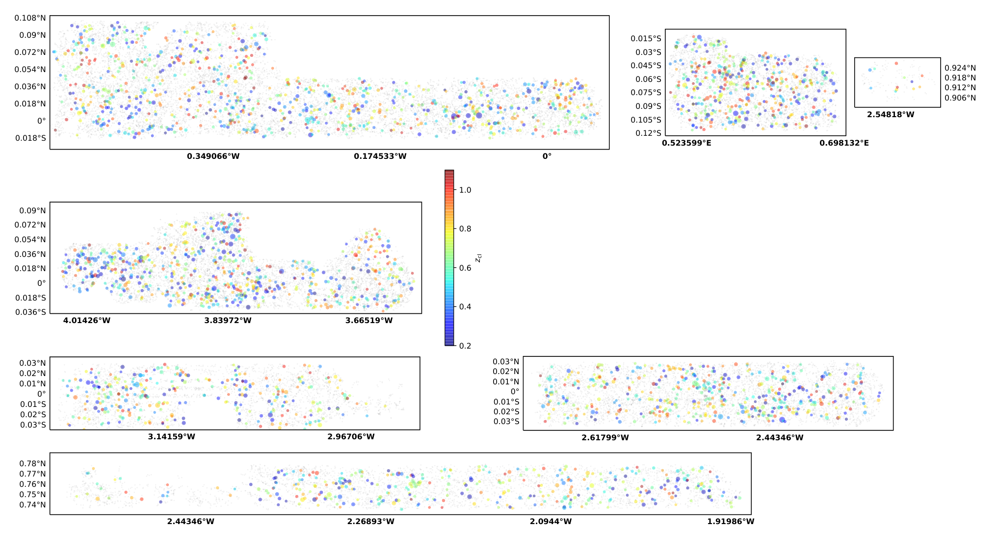
In this work, we use the CAMIRA cluster catalog in the Full-Depth-Full-Color (FDFC) footprint of the HSC WIDE layer with area of $\approx 427$ deg² (after applying the bright star mask). In this cluster catalog, we further select the clusters with richness $N\geq 15$ at redshift $0.2\leq z<1.1$ in the interest of consistency with previous work. Specifically, the cluster sample selected in this criteria was previously studied using weak-lensing shearing (Murata et al. 2019) and magnification (Chiu et al. 2020). Therefore, this choice of the cluster selection enables a direct comparison with the results from gravitational lensing. After the selection in richness and redshift, we further apply the mask of the CMASS galaxy sample (see Section 3.3) that we will cross-correlate with, such that the footprints of the cluster and CMASS samples are identical. This reduces the area to $\approx 403$ deg². As a result, the final cluster sample consists of 3057 systems with $N\geq 15$ at $0.2\leq z<1.1$, which are shown as the points in Figure 1. Their distribution on the sky is shown as in Figure 2. Note that the redshift distribution of CAMIRA clusters is flatter than those of theoretical predictions. This could be explained by a redshift-dependent scatter in richness at fixed mass, as proposed in Murata et al. 2019, where they found that the scatter in richness has a quadratic behavior with the lowest value at the intermediate redshift ($z\approx 0.5$). Higher scatter results in more clusters at given redshift, such that this redshift-dependent scatter produces a flat redshift distribution of clusters. This redshift-dependent scatter was not statistically significant (at a level of $\lesssim 2\sigma$), we therefore do not include this in our modelling of scatter in richness. We leave a more complex modelling of the scatter to the future work.

Given the quality of the HSC data sets, the performance of the photometric redshift ($z_{\mathrm{cl}}$) estimation of CAMIRA clusters is remarkable out to redshift $z\lesssim 1.2$. Specifically, the bias and scatter in terms of $(z_{\mathrm{cl}}-z_{\rm{BCG}})/(1+z_{\rm{BCG}})$ are quantified to be $-0.0013$ and $0.0081$, respectively, where $z_{\rm{BCG}}$ is the observed spectroscopic redshift of the BCGs. In the interest of uniformity, we use the photometric redshift $z_{\mathrm{cl}}$ for each cluster, regardless of available spectroscopic redshifts. We note that a detailed modeling of photo-$z$ uncertainties is needed to correctly interpret observed correlation functions in redshift-space (see Section 2), even with this sub-percent level of precision in the redshift estimation.

We use the spectroscopic sample of galaxies from the Baryon Oscillation Spectroscopic Survey (Dawson et al. 2013, BOSS;), which is the largest survey in the Sloan Digital Sky Survey-III (Eisenstein et al. 2011, SDSS-III;) program. In the BOSS, there are two galaxy samples: LOWZ and CMASS. The LOWZ sample targets the low-redshift galaxy population at $z\lesssim 0.4$, mainly dominated by Luminous Red Galaxies (Eisenstein et al. 2001). On the other hand, the CMASS sample targets galaxies at high redshift of $0.4\lesssim z\lesssim 0.7$, which are pre-selected by using the imaging of the SDSS-II program (Aihara et al. 2011). The target selection in the CMASS sample is based on a combination of customized color and magnitude cuts, such that a sample of galaxies with approximately “constant stellar mass” is expected. We refer readers to Rodríguez-Torres et al. 2016 for more details of the selection of CMASS galaxies.

In this work, we focus on the CMASS sample (in both north and south Galactic Caps) from the Data Release 12 (Alam et al. 2015, DR12;), as the final data release¹¹ 1 https://www.sdss.org/dr15/spectro/lss/#BOSS of the SDSS-III. We only use the regions that are overlapping the S18A FDFC footprint of the HSC survey. Moreover, we carefully apply the bright star mask of the HSC survey to the CMASS catalog, such that the footprints of the CMASS and cluster samples share the same geometry on the sky. The common footprint between the CAMIRA and CMASS samples has area of $\approx 403$ deg², in which about $37k$ CMASS galaxies are present with a median redshift of $z_{\mathrm{BOSS}}=0.57$. The normalized redshift distribution of CMASS galaxies is shown as the red curve in Figure 1. Their distribution on the sky is shown as in Figure 2.

For the random catalog of observed CMASS galaxies, we make use of the random catalogs from both the north and south Galactic Caps that are publicly available²² 2 https://www.sdss.org/dr15/spectro/lss/#BOSS from the DR12. These random catalogs already account for the angular mask of the BOSS. For the random catalogs from both northern and southern hemispheres, we first select the common footprint between the BOSS and HSC survey and then exclude the regions indicated by the HSC masks due to bright stars. Then, we randomly draw a redshift estimate from the observed CMASS sample (with replacements) and assign it to each point in the random catalog, separately for both hemispheres. This is identical to the construction of the CMASS random catalog as in Ross et al. 2012. In the end, the final random catalog for the observed CMASS galaxies is obtained by combining the random catalogs from both northern and southern hemispheres. This process naturally accounts for the difference in the observed redshift distributions between the north and south Galactic Caps.

In this work, we make use of the mock halo catalogs from the N-body simulations in Takahashi et al. 2017 for the tasks of (1) the construction of covariance matrices of the correlation functions, and (2) the end-to-end validation of the codes. We will detail these two tasks in Section 4.2 and Section 5, respectively. In what follows, a brief summary of the mock catalogs is given. We refer readers to Takahashi et al. 2017 for more details of the mock halo catalogs.

A number of 108 full-sky cosmological N-body simulations with high resolution is presented in Takahashi et al. 2017 under a framework of the standard flat $\Lambda\textrm{CDM}$ cosmology with $\Omega_{\mathrm{M}}=0.279$, $\Omega_{\Lambda}=0.721$, $\sigma_{8}=0.82$, and $H_{0}=70\mathrm{km/s}/\mathrm{Mpc}$, which is consistent with the WMAP9 result (Hinshaw et al. 2009). Each set of the N-body simulations is performed using the GADGET2 code (Springel et al. 2001; Springel et al. 2005) in the order of nested cubic boxes around an observer with different box sizes, ranging from $450h^{-1}\mathrm{Mpc}$ to $6300h^{-1}\mathrm{Mpc}$ with a step of $450h^{-1}\mathrm{Mpc}$. Each box contains $2048^{3}$ particles, which corresponds to a particle mass ranging from $\approx 10^{9}h^{-1}\mathrm{M}_{\odot}$ to $\approx 10^{12}h^{-1}\mathrm{M}_{\odot}$, depending on the box side. The resulting matter power spectra of the N-body simulations are fully resolved on the scale of $k<5h\mathrm{Mpc}^{-1}$ at $z<1$ and are in good agreement with the theoretical model predicted by the Halofit (Smith et al. 2003; Takahashi et al. 2012). The dark matter halos are identified by the ROCKSTAR halo finder (Behroozi et al. 2013) with a criterion that the minimal halo mass must be at least 50 times of the particle mass. In this configuration, the resulting mock halo catalogs effectively cover the halo mass range of CMASS galaxies and CAMIRA clusters, by design. In the mass and redshift range of interested in this work, the mass function and the linear halo bias of mock halos are verified to agree with those predicted by the Tinker et al. 2008 and Tinker et al. 2010 formulas within $12\%$ and $10\%$, respectively. In Takahashi et al. 2017, they quantified that the systematic difference in the linear halo bias between the simulated halos and those predicted by the Tinker et al. 2010 fitting formula is at a level of $\lesssim 10\%$ at the wavenumber $k<0.4~h/\mathrm{Mpc}$ ($k<0.1~h/\mathrm{Mpc}$) for $M_{200\mathrm{m}}=10^{13}\mathrm{M}_{\odot}$ ($M_{200\mathrm{m}}=10^{14}\mathrm{M}_{\odot}$) at $z<1.4$ ($z<1.5$). In other words, we expect a systematic uncertainty in the linear halo bias of mock halos at a level of $10\%$ in this work.

With proper rotations of the sky, from each mock catalog we further tile four non-overlapping footprints with the same geometry of the common footprint between the BOSS and HSC survey. This ensures that the four catalogs from the same full-sky simulation are nearly independent with each other on the scale smaller than the current footprint of the survey studied in this work. As a result, we make use of a total number of 432$(=108\times 4)$ mock catalogs that are able to represent the realistic properties, e.g., the mass function and halo clustering, of CMASS galaxies and CAMIRA clusters. From each mock halo catalog among these 432, we further construct a mock catalog of CAMIRA clusters and a mock catalog of CMASS galaxies, as detailed in Section 3.4.1 and Section 3.4.2, respectively.

The two-point auto-correlation function of a tracer $X$, $\xi_{\mathrm{XX}}(s)$ is derived using the Landy & Szalay 1993 estimator, namely

where $\mathrm{X}=\{\mathrm{c},\mathrm{g}\}$ and $\mathrm{c}$ and $\mathrm{g}$ stand for clusters and galaxies, respectively. Here, $\mathrm{D}\mathrm{D}=\mathrm{D}\mathrm{D}(s)$, $\mathrm{D}\mathrm{R}=\mathrm{D}\mathrm{R}(s)$, and $\mathrm{R}\mathrm{R}=\mathrm{R}\mathrm{R}(s)$ are the normalized numbers of pairs with a separation of the redshift-space distance $s$ between the data-data, data-random, and random-random catalogs, respectively. This estimator given by equation (7) can be generalized for the cross-correlation $\xi_{\mathrm{XY}}(s)$ as

where $\mathrm{D_{X}}\mathrm{D_{Y}}$, $\mathrm{D_{X}}\mathrm{R_{Y}}$, $\mathrm{R_{X}}\mathrm{D_{Y}}$, and $\mathrm{R_{X}}\mathrm{R_{Y}}$ are, respectively, the normalized numbers of data-data, data-random, random-data, and random-random pairs found at a separation of $s$ for tracers $\mathrm{X}$ and $\mathrm{Y}$. All tasks of pair counting in this work is done by using TreeCorr (Jarvis et al. 2004).

Using equation (7) and (8), we derive the following correlation functions in this work:

1. 1.

   $\xi_{\mathrm{cc}}$: the auto-correlation of CAMIRA clusters,

2. 2.

   $\xi_{\mathrm{gg}}$: the auto-correlation of CMASS galaxies, and

3. 3.

   $\xi_{\mathrm{c}\mathrm{g}}$: the cross-correlation between CAMIRA clusters and CMASS galaxies.

The correlation functions of $\xi_{\mathrm{cc}}$, $\xi_{\mathrm{c}\mathrm{g}}$ and $\xi_{\mathrm{gg}}$ are estimated in the redshift-space distance $s$ between $10~h^{-1}\mathrm{Mpc}$ and $60~h^{-1}\mathrm{Mpc}$ with logarithmic binning of 7 steps.

Except treating the CAMIRA clusters as a whole in calculating (i) and (iii), we also perform a “subsample” analysis to further investigate the clustering properties as functions of richness and redshift. Namely, we split the cluster sample into two redshift bins ($0.2\leq z<0.7$ and $0.7\leq z<1.1$) and two richness bins ($15\leq N<25$ and $N\geq 25$), with four subsamples in total. Then, we re-measure the clustering functions (i) and (iii) independently for each subsample.

Covariance matrices are needed for statistical analyses because different bins of the observed correlation functions are strongly correlated. By taking the advantage of the large sizes of N-body simulations, we derive covariance matrices based on the 432 mock halo catalogs, which are described in Section 3.4.

We first repeat the measurements ($\xi_{\mathrm{cc}}$, $\xi_{\mathrm{c}\mathrm{g}}$, and $\xi_{\mathrm{gg}}$) on each mock catalogs. In this way, we generate 432 sets of the measurements in the identical configuration as the data. Then, for any combination of a data vector, denoted as $\mathfrak{D}$, we can find the corresponding measurements ${\mathfrak{D}}_{(i)}$ from the $i$-th mock catalog and derive the covariance matrix as

where $\mathfrak{D}_{(\cdot)}=\frac{1}{N_{\mathrm{mock}}}\sum_{i=1}^{N_{\mathrm{mock}}}{\mathfrak{D}}_{(i)}$, and $N_{\mathrm{mock}}=432$. The resulting covariance matrix normalized by the diagonal elements, $\mathfrak{C}_{ij}/(\mathfrak{C}_{ii}\cdot\mathfrak{C}_{jj})^{1/2}$, is shown in Figure 3. We found that the diagonal term of covariance matrices are stable after the number of realizations exceeds $\approx 150$, suggesting that our covariance matrices are converged at the current amount of realizations (i.e, 432).

We further multiply a factor of $\frac{N_{\mathrm{mock}}-N_{\mathrm{D}}-2}{N_{\mathrm{mock}}-1}$, where $N_{\mathrm{D}}$ is the length of a data vector, to the inverse covariance matrix $\mathfrak{C}^{-1}$ to account for the underestimation of the uncertainty because of a finite number of realizations used in estimating the covariance matrix (Hartlap et al. 2007). In this work, the correction factor, $\frac{N_{\mathrm{mock}}-1}{N_{\mathrm{mock}}-N_{\mathrm{D}}-2}$, ranges from $\approx 1.9\%$ (for the modeling of a correlation function of the whole sample; $N_{\mathrm{D}}=7$) to $\approx 17\%$ (for a joint modeling of the auto- and cross-correlation functions in the “subsample” analysis; $N_{\mathrm{D}}=7\times 4~\mathrm{subsamples}\times\left(1~\mathrm{CAMIRA~auto}+1~\mathrm{cross}\right)+7\times\left(1~\mathrm{CMASS~auto}\right)=63$).

In this study, we assume a Gaussian function for the nonlinear smearing effect due to the line-of-sight velocity dispersion, $\sigma_{v}$, as

where

This model is supported by our mocks, in which the distribution of peculiar velocity along the line of sight indeed can be well described as a Gaussian distribution. Figure 4 shows the distribution of the line-of-sight peculiar velocity of mock CMASS galaxies, which is well characterized by a Gaussian distribution with the best-fit dispersion of $\sigma_{v}=310$ km/s. We have carefully checked that the final result is not affected by the choice of the functional form of $G_{v}$ because we analyze the clustering data only on large scales, $s>10$ Mpc$/h$. For clusters for which only photo-$z$ data are available, not only the nonlinear velocity dispersion is smaller than that for galaxies but also the effect of photo-$z$ uncertainties is much severer. Thus, this term can be ignored for our CAMIRA cluster sample (see Section 2).

We model the dispersion $\sigma_{\Delta z}$ of photo-$z$ uncertainties in equation (5) by a Gaussian distribution, described as

where

following equation (6). This is a reasonable assumption, given that the measurement uncertainty of photo-$z$ is indeed distributed as a Gaussian in our work. Thus, $G_{v}$ and $G_{z}$ eventually have the same functional form.

We derive the dispersion $\sigma_{\Delta z}$ of photo-$z$ uncertainties $\Delta z$ for CAMIRA clusters as follows. We assume that cosmological redshift, $z_{\mathrm{c}}$, is identical to the redshift of the BCG, $z_{\mathrm{BCG}}$, ignoring peculiar velocity as a subdominant factor. That is, $\Delta z\equiv z_{\mathrm{cl}}-z_{\mathrm{c}}=z_{\mathrm{cl}}-z_{\mathrm{BCG}}$. Next, we model $\sigma_{\Delta z/\left(1+z_{\mathrm{BCG}}\right)}$ using a power law of cluster richness:

with two free parameters $(\delta_{z},\Gamma_{z})$ that can be constrained from the data. Specifically, we bin CAMIRA clusters in seven richness bins, in which the photo-$z$ uncertainty in terms of $\Delta z/(1+z_{\rm{BCG}})$ in the richness bin ${N}_{i}$ is modeled by a Gaussian distribution with the dispersion of $\sigma_{\Delta z/\left(1+z_{\mathrm{BCG}}\right)}({N}_{i})$ where $i=1,\cdots,7$. Then, we fit equation (16) to the derived data points of $\sigma_{\Delta z/\left(1+z_{\mathrm{BCG}}\right)}({N}_{i})$ over all richness bins. We show the best fit of equation (16) together with the data points in the left panel of Figure 5, with the best-fit parameters,

Note that we use $1165$, out of the $3057$ CAMIRA clusters, that have BCGs with available spectroscopic redshifts $z_{\mathrm{BCG}}$ to determine equation (16). Note that the usage of the functional form in equation (16) is supported by Sereno et al. 2015, in which they studied a sample of clusters with a much larger size and found that the dispersion $\sigma_{\Delta z}$ indeed distributes as a power-law function of richness.

On the other hand, we do not observe a monotonic redshift dependence in $\sigma_{\Delta z/\left(1+z_{\mathrm{BCG}}\right)}$ as seen in the right panel of Figure 5. Rather, the value is roughly a constant, $\sigma_{\Delta z/(1+z_{\rm{BCG}})}\approx 0.009$, and shows a dip at $z\approx 0.4$. This is in great agreement with Murata et al. 2019, where larger dispersion at both low ($z\lesssim 0.4$) and high ($z\gtrsim 0.6$) redshifts was seen than that at $z\approx 0.45$. The larger dispersion at high redshift is expected, because photometry measurements of distant galaxies are noisier. Meanwhile, larger dispersion at low redshift is mainly due to the lack of $u$-band data, as well as a difficulty in estimating the accurate color of close galaxies that are sometimes too bright for the HSC survey (Murata et al. 2019). Additionally, high-richness clusters are more abundant at low redshift than at high redshift (see Figure 1), which could result in a redshift dependence in the best-fit parameters of $(\delta_{z},\Gamma_{z})$. Ideally, the photo-$z$ dispersion should be modeled as a function of both richness and redshift. In this work, however, we cannot simultaneously constrain the richness- and redshift-dependence of the photo-$z$ dispersion, due to the lack of a large spec-$z$ sample. We thus ignore the redshift dependence of $\sigma_{\Delta z/\left(1+z_{\mathrm{BCG}}\right)}$ in this work. The number-weighted average of the richness- and redshift-dependent $\sigma_{\Delta z/(1+z_{\rm{BCG}})}$ over the whole sample is $0.0092$ and $0.0098$, respectively. To first-order approximation, this corresponds to an increase at a level of 0.0006 ($=0.0098-0.0092$) if accounting for the redshift dependence in $\sigma_{\Delta z/(1+z_{\rm{BCG}})}$. A larger spec-$z$ sample is clearly warranted for future work with a detailed modeling of $\sigma_{\Delta z/\left(1+z_{\mathrm{BCG}}\right)}$.

For the CMASS sample, the term $\sigma_{\Delta z}$ is a subdominant factor, given that their redshifts are secured by spectroscopic observations with negligible measurement uncertainties. We thus ignore the measurement uncertainty of the redshift of CMASS galaxies.

In this work, we model the halo bias of CMASS galaxies by a free parameter, $b_{\rm g}=b_{\mathrm{CMASS}}$. This approach is identical to that in Chuang et al. 2013 and is sufficient for CMASS galaxies, in which the redshift-dependence of halo bias is not expected at this narrow range of redshift (Guo et al. 2013). Meanwhile, the halo bias of CAMIRA clusters, $b_{\rm c}$, is linked to their cluster mass based on the Tinker et al. 2010 fitting formula. Additionally, we account for the projection effect on the halo bias of CAMIRA clusters by following the method introduced in Baxter et al. 2016. In what follows, we briefly describe the modeling of the projection effect and refer interested readers to Baxter et al. 2016 for more details.

The projection effect is referred to that a single cluster is due to a projection of multiple systems aligning on the same sky position. We only consider the projection of two halos because the projection of more than two systems is extremely rare and is therefore subdominant (Baxter et al. 2016). Specifically, the halo bias $b_{\mathrm{h}}$ of a cluster at redshift $z$ with an observed richness $N$ is modeled by an effective halo bias $b_{\mathrm{model}}$, as a linear combination of the halo bias without projection, $b^{\mathrm{non-proj}}(N,z)$, and that due to projection, $b^{\mathrm{proj}}(N,z)$. That is,

where $f$ is the probability that the cluster is a product of a projection effect⁵⁵ 5 The parameter $f$ needs to be distinguished from the growth rate parameter $f_{\rm m}$.. The non-projected bias $b^{\mathrm{non-proj}}(N,z)$ is expressed as

where $b_{\mathrm{T10}}$ is the Tinker et al. 2010 halo bias, $N_{\mathrm{M}}(M_{500},z)$ is the mass function evaluated by using the fitting formula in Bocquet et al. 2016, and the term $P(N|M_{500},z,\mathbf{p}_{\mathrm{sr}})$ with the $N$–$M$ parameters $\mathbf{p}_{\mathrm{sr}}$ describes the probability of observing the richness $N$ given the cluster true mass $M_{500}$ at the redshift $z$. We stress that the form of equation (18) already accounts for the Eddington and Malmquist bias, as proved and widely used in previous work (Liu et al. 2015; Chiu et al. 2016; Chiu et al. 2018; Bulbul et al. 2019; Chiu et al. 2020, e.g.,).

It is important to note that the information of the $N$–$M$ scaling relation is fully contained in the term $P(N|M_{500},z,\mathbf{p}_{\mathrm{sr}})$, which includes both measurement uncertainties and intrinsic scatter of richness at fixed cluster mass. The $N$–$M$ scaling relation is characterized by the parameter $\mathbf{p}_{\mathrm{sr}}=\left(A_{N},B_{N},C_{N},\sigma_{N}\right)$ as

with log-normal intrinsic scatter $\sigma_{N}$ at fixed mass, where $B_{N}$ and $C_{N}$ are the mass and redshift power-law indices, respectively; $A_{N}$ is the normalization at the pivotal mass $M_{\mathrm{piv}}=10^{14}h^{-1}\mathrm{M}_{\odot}$ and the pivotal redshift $z_{\mathrm{piv}}=0.6$.

As for the projected halo bias $b^{\mathrm{proj}}$, it reads

in which tilde put on mass $M$ stands for

where $g$ and $q$ are two nuisance parameters over the ranges of $0\leq g\leq 1$ and $0.5\leq q\leq 1$, respectively.

The scenario described by equation (21) is as follows. In a projected system consisting of two halos with mass $M_{1}$ and $M_{2}$, respectively, the halo bias of the projected system is confined to be between those inferred by $M_{1}$ and $M_{1}+M_{2}$ with a definition of $M_{1}>M_{2}$. Then, it is easy to write the halo bias of a projected system as

where $g$ is the nuisance parameter over the range of $0\leq g\leq 1$. Assuming that the projected system is observed with a richness $N$, in which the two halos with mass $M_{1}$ and $M_{2}$ have the richness of ${N}_{1}=qN$ and ${N}_{2}=(1-q)N=\frac{(1-q)}{q}{N}_{1}$ with $0.5\leq q\leq 1$, respectively, we can obtain equation (21) by substituting $M_{2}=\left(\frac{1-q}{q}\right)^{\frac{1}{B_{N}}}M_{1}$ in equation (22) using the relation of $N\sim M^{B_{N}}$ or $M\sim N^{\frac{1}{B_{N}}}$. In a limit of either no projection effect ($q=1$), or zero separation of two halos in a projected system ($q<1$ and $g=1$), equation (20) reduces to equation (18).

Despite quite complex forms of equation (20) and (21), the physical interpretation is rather straightforward: In a two-halo projected system with an observed richness $N$, the projection effect leads to an increasing halo bias of the main sub-halo with respect to that without projection. As a result, this is equivalent to a shift by a factor of $g\left(\frac{1-q}{q}\right)^{\frac{1}{B_{N}}}$ in $b_{\mathrm{T10}}$ given the richness ${N}_{1}=qN$ of the main sub-halo in equation (20).

There are two assumptions implicitly made in modeling the projection effect. First, we assume that observed richness at fixed cluster mass has no dependence on redshift. This assumption is supported by various weak-lensing studies, suggesting that the redshift-trend power-law index $C_{N}$ of richness at fixed cluster mass is indeed consistent with zero (Murata et al. 2019; Chiu et al. 2020, e.g., ). Second, in the model of a two-halo projected system, we assume that these two halos are located at the same redshift $z$ with a negligible redshift separation. This is because a typical redshift separation of subhalos is at $\Delta z\approx 0.02$, which is much smaller than the width of our redshift binning and thus is negligible (Baxter et al. 2016).

The modeling of the projection effect in a greater depth requires an end-to-end validation based on large simulations (Costanzi et al. 2019a; Sunayama et al. 2020, see e.g.,), which is not available for our CAMIRA cluster sample. However, the recent study of Sunayama et al. 2020 suggests that a red-sequence based cluster finder could result in a cluster sample that preferentially selects systems locating at filaments aligning along the line of sight. This selection bias changes the underlying mass distribution of optically selected cluster samples and ultimately bias their clustering measurements. This selection bias is not included in our current modeling of the projection effect, which only accounts for the mis-match between observed richness and underlying true halo mass. We refer readers to Section 7 for more discussions about the selection bias suggested by Sunayama et al. 2020.

Based on the formulation presented in Sections 5.1 to 5.3, we further express the three power spectra in equation (5) for modeling $\xi_{\mathrm{cc}}$, $\xi_{\mathrm{c}\mathrm{g}}$, and $\xi_{\mathrm{gg}}$. They are explicitly given by

where the nonlinear velocity dispersion of CAMIRA clusters and the photo-$z$ uncertainty of CMASS galaxies are ignored (see sections 5.1 and 5.2, respectively). The growth rate $\mathfrak{f_{\mathrm{m}}}=\mathfrak{f_{\mathrm{m}}}(z)$ is evaluated at the median redshift of a given sample, $z_{\rm c}$ and $z_{\rm g}$ for CAMIRA clusters and CMASS galaxies, respectively.

The nonlinear velocity dispersion of CMASS galaxies, $\sigma_{v\mathrm{LoS}}$, is computed as

where the line-of-sight velocity dispersion $\sigma_{v,z_{\rm g}}$ of CMASS galaxies is fixed to $310~\mathrm{km}/\mathrm{sec}$, as suggested by our mocks (see Section 5.1). Note that we fix $z_{\mathrm{g}}$ to $0.57$, as the median redshift of the CMASS sample.

Given a sample of CAMIRA clusters with a set of observed richness $N$, $\sigma_{z\mathrm{LoS}}$ is computed as in equation (15),

where $\overline{\sigma_{\Delta z}}$ is evaluated as the mean value of $\sigma_{\Delta z}(N)$ (i.e., equation (16)) among the clusters in the sample, given a set of parameters $\left(\delta_{z},\Gamma_{z}\right)$. We use the cluster photo-$z$ in evaluating $\overline{\sigma_{\Delta z}}$.

The linear halo bias of CMASS galaxies, $b_{\rm g}=b_{\mathrm{CMASS}}$, is the only free parameter to model the amplitude of $\xi_{\mathrm{gg}}$. The remaining quantity is the halo bias of CAMIRA clusters, $b_{\rm c}$, which is linked to the cluster mass and further connected to the observable (i.e., richness) by the $N$–$M$ scaling relation. In this way, one can calibrate the $N$–$M$ parameters by forward-modeling to an observed correlation function. This process is referred to as the “self-calibration” of the $N$–$M$ relation based on clustering alone. The halo bias of CAMIRA clusters is modeled as the mean value of the cluster sample, namely, $b_{\rm c}=\overline{b_{\mathrm{model}}}$, where $\overline{b_{\mathrm{model}}}$ is the mean value of $b_{\mathrm{model}}\left(N,z\right)$ given by equation (17) over the cluster sample, given a set of parameters $\left(A_{N},B_{N},C_{N},\sigma_{N},f,g,q\right)$. It is worth mentioning that the we use the same cluster halo bias $b_{\rm c}$ in modelling both $\xi_{\mathrm{cc}}$ and $\xi_{\mathrm{c}\mathrm{g}}$, while the clustering signals of the latter are dominated by the cluster-galaxy pairs at the range of overlapping redshift ($0.4\lesssim z\lesssim 0.7$). We have verified that using a subsample of CAMIRA clusters, which are selected based on their redshifts such that the redshift distribution of clusters follows that of CMASS galaxies, to calculate $b_{\rm c}$ in modelling $\xi_{\mathrm{c}\mathrm{g}}$ results in negligible difference.

To sum up, we will have nine free parameters, $\mathbf{p}=\left\{A_{N},B_{N},C_{N},\sigma_{N},f,g,q,\delta_{z},\Gamma_{z}\right\}$, in modeling $\xi_{\mathrm{cc}}$. The first fourth parameters characterize the $N$–$M$ relation. The parameters of $f$, $g$, and $q$ are used to model the projection effect, while the last two ($\delta_{z}$ and $\Gamma_{z}$) describe the redshift-smearing effect due to the photo-$z$ uncertainty of CAMIRA clusters. The self-calibration of the $N$–$M$ relation is performed by modeling $\xi_{\mathrm{c}\mathrm{g}}$ with an additional parameter of the CMASS halo bias $b_{\mathrm{CMASS}}$ on top of the nine free parameters above, and thus we have ten free parameters for the modeling of the cross-correlation function.

In this subsection, we describe the forward-modeling approach to calibrate the $N$–$M$ relation by modeling the measurements of auto- and/or cross-correlation functions in a framework of fixed cosmology.

We explore the parameter space using emcee (Foreman-Mackey et al. 2013; Foreman-Mackey et al. 2019), which implements the Affine Invariant Markov Chain Monte Carlo (MCMC) algorithm. For a given data vector $\mathfrak{D}$ and the parameter vector $\mathbf{p}$, the posterior $\mathfrak{P}(\mathbf{p}|\mathfrak{D})$ of $\mathbf{p}$ is expressed as

where $\mathcal{P}$ is the prior on $\mathbf{p}$, and $\mathcal{L(\mathfrak{D}|\mathbf{p})}$ is the likelihood of the model evaluated with the parameter vector $\mathbf{p}$. The log-likelihood $\ln\mathcal{L(\mathfrak{D}|\mathbf{p})}$ reads

where $\mathfrak{C}$ is the covariance matrix defined in Section 4.2, and $\mathfrak{M}$ is the model of auto- and/or cross-correlation functions corresponding to the data vector $\mathfrak{D}$ (see Section 5). The matter power spectra $P_{\mathrm{m}}(k)$ in equations (23) and (5.4) are evaluated at the mean redshift of CAMIRA clusters in the sample (or the subsample).

Note that $\mathfrak{D}$ represents a generic term of data vectors, which can be a combination of various auto- and cross-correlation functions measured in the whole sample or different subsamples of richness and redshift. In this work, we perform the modeling of $\xi_{\mathrm{cc}}$, $\xi_{\mathrm{c}\mathrm{g}}$, and $\xi_{\mathrm{gg}}$ separately, and the joint modeling of $\xi_{\mathrm{cc}}+\xi_{\mathrm{c}\mathrm{g}}$ and $\xi_{\mathrm{cc}}+\xi_{\mathrm{c}\mathrm{g}}+\xi_{\mathrm{gg}}$. For fitting the $\xi_{\mathrm{cc}}$ alone, we have nine free parameters, $\mathbf{p}=\left\{A_{N},B_{N},C_{N},\sigma_{N},f,g,q,\delta_{z},\Gamma_{z}\right\}$. For modeling $\xi_{\mathrm{gg}}$ alone, as the simplest case, there is only one free parameter, the halo bias $b_{\rm{CMASS}}$. If a cross-correlation function ($\xi_{\mathrm{c}\mathrm{g}}$) is included in the modeling, then we have ten free parameters, $\mathbf{p}=\left\{A_{N},B_{N},C_{N},\sigma_{N},f,g,q,\delta_{z},\Gamma_{z},b_{\mathrm{CMASS}}\right\}$.

In this work, we cannot meaningfully constrain all parameters at the same time without informative priors, given current measurement uncertainties as well as the degeneracy among parameters. Therefore, we focus on constraining the normalization $A_{N}$ of the $N$–$M$ relation while applying the informative priors on other parameters. Specifically, we apply Gaussian priors of $\mathcal{N}(0.92,0.13^{2})$, $\mathcal{N}(-0.48,0.69^{2})$, and $\mathcal{N}(0.15,0.07^{2})$ on $B_{N}$, $C_{N}$, and $\sigma_{N}$, respectively. These priors are suggested by the posteriors independently constrained by lensing magnification (Chiu et al. 2020) and are statistically consistent with those obtained by a joint analysis of weak shear and cluster abundance (Murata et al. 2019). Only a uniform prior between $0$ and $100$ is applied on $A_{N}$.

A Gaussian prior $\mathcal{N}(0.1,0.05^{2})$ is applied on the parameter $f$ with an additional requirement of $0\leq f\leq 1$ to describe the percentage of projected systems in the sample. This value is suggested by another optically selected cluster sample in the SDSS (Baxter et al. 2016; Simet et al. 2017). Flat priors of $\mathcal{U}(0,1)$ and $\mathcal{U}(0.5,1)$ are applied on $g$ and $q$, respectively. Note that we cannot well constrain the parameters of $f$, $g$, and $q$ based on cluster clustering alone, for which a dedicated effort using large simulations is needed (Costanzi et al. 2019a, e.g.,) and is currently not available for our sample. By applying these priors in a MCMC framework, we effectively marginalize these parameters over the range of the parameter space with a minimal requirement of informative knowledge. For the parameters of $\delta_{z}$ and $\Gamma_{z}$, we apply Gaussian priors of $\mathcal{N}(0.0093,0.0002^{2})$ and $\mathcal{N}(-0.18,0.05^{2})$, which are suggested by our data (see Section 5.2), respectively.

The halo bias $b_{\mathrm{CMASS}}$ is varied with a Gaussian prior $\mathcal{N}(1.93,0.17^{2})$, which was the posterior independently constrained by RSD and BAO together with the WMAP9 CMB data (Chuang et al. 2013). Although different cosmological parameters are used and fixed in this work, we note that the constraint of $b_{\mathrm{CMASS}}$ in Chuang et al. 2013 takes into account the variation of cosmological parameters and serves an adequate prior here. We stress that the strategy in this work is to leverage the clustering of CMASS galaxies to improve the constraints on the mass calibration of CAMIRA clusters; therefore, imposing an informative prior on $b_{\mathrm{CMASS}}$ from an BAO analysis in the modelling of $\xi_{\mathrm{c}\mathrm{g}}$ is a reasonable approach. However, we note that the Gaussian prior on $b_{\mathrm{CMASS}}$ is not informative, once the measurement of $\xi_{\mathrm{gg}}$ is included in the modelling. This is because the constraining power on $b_{\mathrm{CMASS}}$ based on $\xi_{\mathrm{gg}}$ alone is significantly stronger than the imposed prior. In this case, removing the informative prior on $b_{\mathrm{CMASS}}$ results in negligible difference to that with the prior. In the interest of a uniform analysis in this work, however, we still consistently apply the Gaussian prior on $b_{\mathrm{CMASS}}$ in all modelling, even those including $\xi_{\mathrm{gg}}$. A summary of the adopted priors is given in Table 1.

By using the mock catalogs, we perform end-to-end validation tests of our codes and the assumptions made in the modeling. For example, in this work we assume that the power spectrum can be simply described by equation (5), which only models the effects of the RSD, FoG, and photo-$z$ smearing without accounting for, e.g., the assembly bias (Lin et al. 2016; Zu et al. 2017). By carrying out the modeling on mock measurements in the identical way as on the data, our goal is to ensure that we can recover the input parameters $(A_{N},B_{N},C_{N},\sigma_{N})$ of the $N$–$M$ scaling relation without significant bias.

To do so, we randomly draw 10 different sets of mock measurements to enlarge the sample size in mock modeling, such that the bias (if exists) would not be hidden by statistical uncertainties, which are $3.2\left(\approx\sqrt{10}\right)$ times smaller than those of the observations. For a combination of data vectors in equation (28), the posteriors of the parameters in the joint modeling of the mock measurements are

where $\mathfrak{D_{i}}$ is the $i$-th mock measurement.

Despite the efforts in carefully mimicking observational properties of CAMIRA clusters and CMASS galaxies in the mock catalogs, we note some of the limitations of the mocks. First, the redshift estimates of mock catalogs only contain measurement uncertainties, distributed as a Gaussian distribution, but not the systematics introduced by the CAMIRA cluster finder. This inevitably results in a moderate discrepancy in the redshift distribution between the mocks and the real data. Second, we change the mean of the Gaussian prior on $b_{\mathrm{CMASS}}$ from $1.93$ to $1.71$, which is the median value of the CMASS halo bias evaluated using the true halo mass following the Tinker et al. 2010 formula. Given the systematic uncertainty in the halo bias of mock halos at a level of $10\%$ (see Section 3.4), this value is statistically consistent ($\lesssim 1\sigma$) with the observational constraint from Chuang et al. 2013. Third, we still simultaneously model the parameters of $(f,g,q)$ in the identical way as described in Section 5.4, although there is no projection effect on the halo bias of mock clusters. Fourth, there is no selection bias in mock cluster catalogs, as opposed to the real data. It has been suggested that a selection bias could exist in a cluster sample constructed by a red-sequence based algorithm (Sunayama et al. 2020), such as CAMIRA. We refer readers to Section 7 for more discussions about this selection bias. Fifth, the $N$–$M$ relation in mock cluster catalogs is assumed to have log-normal intrinsic scatter of richness at fixed mass. It is worth mentioning that a redshift-dependent form for intrinsic scatter is suggested for CAMIRA clusters, although without statistically significant evidence (Murata et al. 2019).

The results of the mock validations are shown in Figure 6, where we show the constraints of the parameters from the modeling of $\xi_{\mathrm{cc}}$, $\xi_{\mathrm{c}\mathrm{g}}$, and $\xi_{\mathrm{gg}}$, independently, and the combination among them. As seen in Figure 6, our modeling can recover the input parameters (within $1\sigma$), indicated by the dashed lines. This suggests that (1) our modeling approach can deliver an unbiased result, and that (2) the assumptions made in constructing the models are valid. We further show the best-fit profiles and the mock measurements in Figure 7, demonstrating that our models provide a good description of the measurements. Note that the mock validations on the subsample analysis deliver the same picture as the default analysis, we thus only present the results of mock validations using the cluster sample as a whole.

It is interesting to note that the constraint on the normalization $A_{N}$ in modeling $\xi_{\mathrm{c}\mathrm{g}}$ alone is weaker than that in modeling $\xi_{\mathrm{cc}}$ alone. This is due to a strong degeneracy between the normalization $A_{N}$ and the CMASS halo bias $b_{\mathrm{CMASS}}$, which is completely dominated by the prior. Consequently, the constraint on $A_{N}$ largely depends on the prior on $b_{\mathrm{CMASS}}$ and becomes weaker than that from modeling $\xi_{\mathrm{cc}}$ alone. On the other hand, the joint modeling of $\xi_{\mathrm{cc}}$ and $\xi_{\mathrm{c}\mathrm{g}}$ (shown in green) shows that the constraint on $A_{N}$ completely follows that in the modeling of $\xi_{\mathrm{cc}}$ alone (shown in blue), effectively breaking the $A_{N}$-$b_{\mathrm{CMASS}}$ degeneracy. Meanwhile, the inclusion of $\xi_{\mathrm{gg}}$ in the joint modeling (shown in brown) essentially pins down the CMASS halo bias $b_{\mathrm{CMASS}}$, resulting in an absolute calibration of $A_{N}$ with slightly better accuracy and precision.

To sum up, we conclude that our modeling strategies can recover the underlying true values of the parameters within uncertainties, as suggested by our end-to-end mock validations.

References

- Aihara et al. (2011) Aihara H. et al., 2011, ApJS, 193, 29
- Aihara et al. (2019a) Aihara H. et al., 2019a, PASJ, 71, 114
- Aihara et al. (2019b) Aihara H. et al., 2019b, PASJ, 71, 114
- Aihara et al. (2018a) Aihara H. et al., 2018a, PASJ, 70, S4
- Aihara et al. (2018b) Aihara H. et al., 2018b, PASJ, 70, S8
- Alam et al. (2015) Alam S. et al., 2015, ApJS, 219, 12
- Astropy Collaboration et al. (2013) Astropy Collaboration et al., 2013, A&A, 558, A33
- Bahcall et al. (2003) Bahcall N. A., Dong F., Hao L., Bode P., Annis J., Gunn J. E., Schneider D. P., 2003, ApJ, 599, 814
- Baxter et al. (2016) Baxter E. J., Rozo E., Jain B., Rykoff E., Wechsler R. H., 2016, MNRAS, 463, 205
- Behroozi et al. (2013) Behroozi P. S., Wechsler R. H., Wu H.-Y., Busha M. T., Klypin A. A., Primack J. R., 2013, ApJ, 763, 18
- Bocquet & Carter (2016) Bocquet S., Carter F. W., 2016, The Journal of Open Source Software, 1, 46
- Bocquet et al. (2019) Bocquet S. et al., 2019, ApJ, 878, 55
- Bocquet et al. (2016) Bocquet S., Saro A., Dolag K., Mohr J., 2016, MNRAS, 456, 2361
- Bocquet et al. (2015) Bocquet S. et al., 2015, ApJ, 799, 214
- Bosch et al. (2018) Bosch J. et al., 2018, PASJ, 70, S5
- Bulbul et al. (2019) Bulbul E. et al., 2019, ApJ, 871, 50
- Chambers et al. (2016) Chambers K. C. et al., 2016, arXiv e-prints, arXiv:1612.05560
- Chiu et al. (2018) Chiu I. et al., 2018, MNRAS, 478, 3072
- Chiu et al. (2016) Chiu I. et al., 2016, MNRAS, 458, 379
- Chiu et al. (2020) Chiu I. N., Umetsu K., Murata R., Medezinski E., Oguri M., 2020, MNRAS, 495, 428
- Chuang et al. (2013) Chuang C.-H. et al., 2013, MNRAS, 433, 3559
- Collins et al. (2000) Collins C. A. et al., 2000, MNRAS, 319, 939
- Costanzi et al. (2019a) Costanzi M. et al., 2019a, MNRAS, 482, 490
- Costanzi et al. (2019b) Costanzi M. et al., 2019b, MNRAS, 488, 4779
- Coupon et al. (2018) Coupon J., Czakon N., Bosch J., Komiyama Y., Medezinski E., Miyazaki S., Oguri M., 2018, PASJ, 70, S7
- Dawson et al. (2013) Dawson K. S. et al., 2013, AJ, 145, 10
- de Haan et al. (2016) de Haan T. et al., 2016, ApJ, 832, 95
- DESI Collaboration et al. (2016) DESI Collaboration et al., 2016, arXiv e-prints, arXiv:1611.00036
- Dietrich et al. (2019) Dietrich J. P. et al., 2019, MNRAS, 483, 2871
- Eisenstein et al. (2001) Eisenstein D. J. et al., 2001, AJ, 122, 2267
- Eisenstein et al. (2011) Eisenstein D. J. et al., 2011, AJ, 142, 72
- Emami et al. (2017) Emami R. et al., 2017, arXiv e-prints, arXiv:1711.05210
- Estrada et al. (2009) Estrada J., Sefusatti E., Frieman J., 2009, ApJ, 692, 265
- Foreman-Mackey et al. (2019) Foreman-Mackey D. et al., 2019, The Journal of Open Source Software, 4, 1864
- Foreman-Mackey et al. (2013) Foreman-Mackey D., Hogg D., Lang D., Goodman J., 2013, PASP, 125, 306
- Furusawa et al. (2018) Furusawa H. et al., 2018, PASJ, 70, S3
- Guo et al. (2018) Guo H., Yang X., Lu Y., 2018, ApJ, 858, 30
- Guo et al. (2013) Guo H. et al., 2013, ApJ, 767, 122
- Hartlap et al. (2007) Hartlap J., Simon P., Schneider P., 2007, A&A, 464, 399
- Hinshaw et al. (2009) Hinshaw G. et al., 2009, ApJS, 180, 225
- Hinton (2016) Hinton S. R., 2016, The Journal of Open Source Software, 1, 00045
- Hoekstra et al. (2015) Hoekstra H., Herbonnet R., Muzzin A., Babul A., Mahdavi A., Viola M., Cacciato M., 2015, MNRAS, 449, 685
- Holder (2006) Holder G., 2006, ArXiv Astrophysics e-prints
- Holder et al. (2001) Holder G., Haiman Z., Mohr J., 2001, ApJ, 560, L111
- Hu & Cohn (2006) Hu W., Cohn J., 2006, Phys. Rev. D, 73, 067301
- Huang et al. (2018) Huang S. et al., 2018, PASJ, 70, S6
- Hunter (2007) Hunter J. D., 2007, Computing In Science & Engineering, 9, 90
- Hütsi (2010) Hütsi G., 2010, MNRAS, 401, 2477
- Ivezic et al. (2008) Ivezic Z. et al., 2008, Serbian Astronomical Journal, 176, 1
- Ivezic et al. (2019) Ivezic Ž. et al., 2019, ApJ, 873, 111
- Jackson (1972) Jackson J. C., 1972, MNRAS, 156, 1P
- Jarvis et al. (2004) Jarvis M., Bernstein G., Jain B., 2004, MNRAS, 352, 338
- Jimeno et al. (2015) Jimeno P., Broadhurst T., Coupon J., Umetsu K., Lazkoz R., 2015, MNRAS, 448, 1999
- Jones et al. (2001) Jones E., Oliphant T., Peterson P., et al., 2001, SciPy: Open source scientific tools for python
- Juric et al. (2017) Juric M. et al., 2017, Astronomical Society of the Pacific Conference Series, Vol. 512, The LSST Data Management System, Lorente N. P. F., Shortridge K., Wayth R., eds., p. 279
- Kaiser (1987) Kaiser N., 1987, MNRAS, 227, 1
- Kawanomoto et al. (2018) Kawanomoto S. et al., 2018, PASJ, 70, 66
- Komiyama et al. (2018) Komiyama Y. et al., 2018, PASJ, 70, S2
- Landy & Szalay (1993) Landy S. D., Szalay A. S., 1993, ApJ, 412, 64
- Laureijs et al. (2011) Laureijs R. et al., 2011, arXiv e-prints, arXiv:1110.3193
- Lima & Hu (2004) Lima M., Hu W., 2004, Phys. Rev. D, 70, 043504
- Lin et al. (2016) Lin Y.-T., Mandelbaum R., Huang Y.-H., Huang H.-J., Dalal N., Diemer B., Jian H.-Y., Kravtsov A., 2016, ApJ, 819, 119
- Liu et al. (2015) Liu J. et al., 2015, MNRAS, 448, 2085
- Magnier et al. (2013) Magnier E. A. et al., 2013, ApJS, 205, 20
- Majumdar & Mohr (2003) Majumdar S., Mohr J., 2003, ApJ, 585, 603
- Mana et al. (2013) Mana A., Giannantonio T., Weller J., Hoyle B., Hütsi G., Sartoris B., 2013, MNRAS, 434, 684
- Mandelbaum et al. (2018) Mandelbaum R. et al., 2018, PASJ, 70, S25
- Mandelbaum et al. (2013) Mandelbaum R., Slosar A., Baldauf T., Seljak U., Hirata C. M., Nakajima R., Reyes R., Smith R. E., 2013, MNRAS, 432, 1544
- Manera et al. (2013) Manera M. et al., 2013, MNRAS, 428, 1036
- Mantz et al. (2015) Mantz A. B. et al., 2015, MNRAS, 446, 2205
- Marulli et al. (2011) Marulli F., Carbone C., Viel M., Moscardini L., Cimatti A., 2011, MNRAS, 418, 346
- McClintock et al. (2019) McClintock T. et al., 2019, MNRAS, 482, 1352
- Merloni et al. (2012) Merloni A. et al., 2012, ArXiv e-prints
- Miyazaki (2015) Miyazaki S., 2015, IAU General Assembly, 22, 2255916
- Miyazaki et al. (2018) Miyazaki S. et al., 2018, PASJ, 70, S1
- Murata et al. (2019) Murata R. et al., 2019, PASJ, 71, 107
- Murata et al. (2020) Murata R., Sunayama T., Oguri M., More S., Nishizawa A. J., Nishimichi T., Osato K., 2020, arXiv e-prints, arXiv:2001.01160
- Oguri (2014) Oguri M., 2014, MNRAS, 444, 147
- Oguri et al. (2018) Oguri M. et al., 2018, PASJ, 70, S20
- Okumura et al. (2015) Okumura T., Hand N., Seljak U., Vlah Z., Desjacques V., 2015, Phys. Rev. D, 92, 103516
- Okumura et al. (2016) Okumura T. et al., 2016, PASJ, 68, 38
- Paech et al. (2017) Paech K., Hamaus N., Hoyle B., Costanzi M., Giannantonio T., Hagstotz S., Sauerwein G., Weller J., 2017, MNRAS, 470, 2566
- Park et al. (1994) Park C., Vogeley M. S., Geller M. J., Huchra J. P., 1994, ApJ, 431, 569
- Peacock & Dodds (1994) Peacock J. A., Dodds S. J., 1994, MNRAS, 267, 1020
- Pérez & Granger (2007) Pérez F., Granger B. E., 2007, Computing in Science and Engineering, 9, 21
- Planck Collaboration et al. (2015) Planck Collaboration P. et al., 2015, Astronomy & Astrophysics, Volume 594, id.A24, 19 pp., 594
- Rodríguez-Torres et al. (2016) Rodríguez-Torres S. A. et al., 2016, MNRAS, 460, 1173
- Ross et al. (2012) Ross A. J. et al., 2012, MNRAS, 424, 564
- Rykoff et al. (2014) Rykoff E. S. et al., 2014, ApJ, 785, 104
- Schlafly et al. (2012) Schlafly E. F. et al., 2012, ApJ, 756, 158
- Schrabback et al. (2018) Schrabback T. et al., 2018, MNRAS, 474, 2635
- Schuecker et al. (2003) Schuecker P., Böhringer H., Collins C. A., Guzzo L., 2003, A&A, 398, 867
- Sereno et al. (2015) Sereno M., Veropalumbo A., Marulli F., Covone G., Moscardini L., Cimatti A., 2015, MNRAS, 449, 4147
- Simet et al. (2017) Simet M., McClintock T., Mandelbaum R., Rozo E., Rykoff E., Sheldon E., Wechsler R. H., 2017, MNRAS, 466, 3103
- Smith et al. (2003) Smith R. et al., 2003, MNRAS, 341, 1311
- Soergel et al. (2016) Soergel B. et al., 2016, MNRAS, 461, 3172
- Springel et al. (2005) Springel V. et al., 2005, Nature, 435, 629
- Springel et al. (2001) Springel V., White S., Tormen G., Kauffmann G., 2001, MNRAS, 328, 726
- Sunayama et al. (2020) Sunayama T. et al., 2020, arXiv e-prints, arXiv:2002.03867
- Takada et al. (2014) Takada M. et al., 2014, PASJ, 66, R1
- Takahashi et al. (2017) Takahashi R., Hamana T., Shirasaki M., Namikawa T., Nishimichi T., Osato K., Shiroyama K., 2017, ApJ, 850, 24
- Takahashi et al. (2012) Takahashi R., Sato M., Nishimichi T., Taruya A., Oguri M., 2012, ApJ, 761, 152
- Tanaka et al. (2018) Tanaka M. et al., 2018, PASJ, 70, S9
- Tanaka et al. (2017) Tanaka M. et al., 2017, arXiv e-prints, arXiv:1706.00566
- Taylor (2005) Taylor M. B., 2005, in Astronomical Society of the Pacific Conference Series, Vol. 347, Astronomical Data Analysis Software and Systems XIV, Shopbell P., Britton M., Ebert R., eds., p. 29
- The Dark Energy Survey Collaboration (2005) The Dark Energy Survey Collaboration, 2005, arXiv e-prints, astro
- The Dark Energy Survey Collaboration et al. (2016) The Dark Energy Survey Collaboration et al., 2016, MNRAS, 460, 1270
- Tinker et al. (2008) Tinker J., Kravtsov A., Klypin A., Abazajian K., Warren M., Yepes G., Gottlöber S., Holz D., 2008, ApJ, 688, 709
- Tinker et al. (2010) Tinker J. L., Robertson B. E., Kravtsov A. V., Klypin A., Warren M. S., Yepes G., Gottlöber S., 2010, ApJ, 724, 878
- Tonry et al. (2012) Tonry J. L. et al., 2012, ApJ, 750, 99
- Umetsu et al. (2014) Umetsu K. et al., 2014, ApJ, 795, 163
- Van Der Walt et al. (2011) Van Der Walt S., Colbert S. C., Varoquaux G., 2011, Computing in Science & Engineering, 13, 22
- von der Linden et al. (2014a) von der Linden A. et al., 2014a, MNRAS, 439, 2
- von der Linden et al. (2014b) von der Linden A. et al., 2014b, MNRAS, 443, 1973
- Wang & Steinhardt (1998) Wang L., Steinhardt P. J., 1998, ApJ, 508, 483
- York et al. (2000) York D. G. et al., 2000, AJ, 120, 1579
- Zu et al. (2017) Zu Y., Mandelbaum R., Simet M., Rozo E., Rykoff E. S., 2017, MNRAS, 470, 551