Scaling equations for mode-coupling theories with multiple decay channels

Let us consider a system of $N$ identical particles, confined in z-direction between two parallel, hard walls Lang et al. 2012. The system can be described by the microscopic particle density,

with $\bm{r}=(x,y)$. Due to translational symmetry in the directions parallel to the walls, we find that the averaged density $\left\langle\rho(\bm{r},z,t)\right\rangle=n(z)$ only depends on the z-coordinate. To characterize the dynamics of the microscopic system we introduce the Van Hove correlation function,

as the time-correlation function of the microscopic density fluctuations, $\delta\rho(\bm{r},z,t)=\rho(\bm{r},z,t)-n(z)$, normalized by the area density $n_{0}$. It is now natural and numerically convenient to introduce density modes as the Fourier transform of the particle density, $\rho_{\mu}(\bm{q},t)=\sum_{i=1}^{N}\exp[{\rm i}Q_{\mu}z_{i}(t)]\exp[{\rm i}\bm{q}\cdot\bm{r}_{i}(t)]$. The modes perpendicular to the confining direction are discrete, $Q_{\mu}=2\pi\mu/L$, in contrast to the continuous wave vectors $\bm{q}$ in the lateral direction. Here, $L$ is the accessible slit width. From this we can define the generalized intermediate scattering function (ISF),

By Fourier transformation one immediately finds that the ISF is nothing but the Fourier transform of the above introduced Van Hove correlation function Lang et al. 2012,

Choosing the density modes $\left\{\rho_{\mu}(\bm{q},t)\right\}$ as set of distinguished variables, the Zwanzig-Mori projection operator formalismZwanzig 2001; Götze 2009; Hansen and McDonald 2006 yields the equations of motion for the intermediate scattering function,

Here, we have introduced the matrix notation $\left[\mathbf{S}(t)\right]_{\mu\nu}=S_{\mu\nu}(q,t)$ and the generalized structure factor $\mathbf{S}=\mathbf{S}(t=0)$. Occasionally the dependence on the wavevector $\bm{q}$ will be suprressed in cases where it serves merely as a parameter. The a priori unknown memory kernel $\left[\mathbf{K}(t)\right]_{\mu\nu}=K_{\mu\nu}(q,t)$ defines the non-Markovian dynamics of the ISF and corresponds formally to the time correlation function of the time derivatives of the density fluctuations, $\dot{\rho}_{\mu}(\bm{q})$ albeit with projected dynamics. More precisely, it is the correlation function of $\dot{\rho}_{\mu}(\bm{q},0)$ with $e^{(1-\mathcal{P})\mathcal{L}t}\dot{\rho}_{\mu}(\bm{q},0)$, where $\mathcal{L}$ is the standard Liouville operator and $\mathcal{P}$ the Zwanzig-Mori projection operator Zwanzig 2001; Götze 2009.

To derive an expression for the memory kernel, we use the fact that the density modes fulfill the continuity equation,

where the superscript $\alpha$ is referred to as channel index and the $q_{\mu}^{\alpha}$ define the fundamental couplings of the current channel $j^{\alpha}_{\mu}(\bm{q},t)$ to the density modes. Since we are interested in systems with multiple relaxation channels, we need to generalize the standard continuity equation such that the currents split into ${m}\in\mathbb{N}$ distinct contributions. In case of the slit geometry the decay channels correspond to the longitudinal and transversal currents and we have, $q_{\mu}^{\alpha}=q\delta_{\alpha\parallel}+Q_{\mu}\delta_{\alpha\perp}$. This splitting is physically motivated since we expect the relaxation dynamics to be significantly different in the directions parallel and orthogonal to the walls. From the above continuity equation we conclude that also the memory kernel naturally splits into multiple decay channels,

Here, the generalized memory kernel $\left[\bm{\mathcal{K}}(t)\right]^{\alpha\beta}_{\mu\nu}=\mathcal{K}_{\mu\nu}^{\alpha\beta}(q,t)$ carries in addition to the mode indices $\mu,\nu$ also the channel indices $\alpha,\beta\in\{1,\ldots,m\}$. Generally, we will denote matrix-valued objects with mode and channel indices by caligraphic letters. The conventional current kernel $\mathbf{K}(t)$ is obtained as contraction $\mathcal{C}\{\bm{\mathcal{K}}(t)\}$ from the generalized current kernel. We can perform a second Zwanzig-Mori projection step using the current modes $\{j_{\mu}^{\alpha}(\bm{q},t)\}$ as distinguished variable and derive evolution equations for the current kernels,

with the static current correlator ${\mathcal{J}}^{\alpha\beta}_{\mu\nu}(q)\coloneqq N^{-1}\left\langle j^{\alpha}_{\mu}(\bm{q},0)^{*}j^{\beta}_{\nu}(\bm{q},0)\right\rangle={\mathcal{K}}^{\alpha\beta}_{\mu\nu}(q,t=0)$. Here, the matrix $\bm{\mathcal{J}}\succ 0$ is positive definite, while the instantaneous damping $\bm{\mathcal{D}}^{-1}\succeq 0$ is positive semidefinite. The new memory kernel $\bm{\mathcal{M}}(t)$ formally corresponds to the correlation functions of generalized forces with the further reduced dynamic time evolution.

The mode-coupling theory approach is now to approximate the force kernel $\bm{\mathcal{M}}(t)$ as a bilinear functional of the intermediate scattering functions,

with,

where the vertices $\mathcal{Y}^{\alpha}_{\mu\mu_{1}\mu_{2}}(\bm{q},\bm{q}_{1},\bm{q}_{2})$ depend on the specific system that is described with this kind of MCT, like confined liquids Lang et al. 2012 or molecules Schilling and Scheidsteger 1997. Here, we only need to assume that the vertices are smooth functions of the control parameters. We will anticipate the thermodynamic limit, however, for the moment we will assume that the wave vectors are discrete. Additionally, both the wave vectors and the modes will be truncated, i.e. the matrices are finite dimensional.

To find a set of integro-differential equations similar to the ones used in previously performed asymptotic analysis for a single decay channel Franosch et al. 1997; Elizondo-Aguilera and Voigtmann 2019 we introduce the Laplace transformation of a time-dependent matrix $\mathbf{A}(t)$,

and rewrite Eqs. (5) and (8),

With this we can define an effective memory kernel, $\mathbf{M}(z)$, as,

with static current correlator $\mathbf{{J}}=\mathbf{K}(t=0)=\mathcal{C}\{\bm{\mathcal{J}}\}\succ 0$ and effective damping matrix $\mathbf{{D}}^{-1}=\mathbf{J}^{-1}\mathcal{C}\{\bm{\mathcal{J}}\bm{\mathcal{D}}^{-1}\bm{\mathcal{J}}\}\mathbf{J}^{-1}\succeq 0$. One can show that $\hat{\mathbf{M}}(z)$ indeed shares all the properties of a matrix-valued correlation function Franosch 2014, in particular, its spectrum is non-negative. Here, it corresponds precisely to the force kernel provided the second Zwanzig-Mori step is performed without splitting the currents.

For the ISF in the time domain we therefore find the standard generalized harmonic oscillator equation for matrix-valued correlation functions,

subject to the initial conditions $\mathbf{S}(t=0)=\mathbf{S},\dot{\mathbf{S}}(t=0)=0$. The introduction of the effective memory kernel, $\mathbf{M}(t)$, proved also useful to derive a stable numerical integrator Chong et al. 2000; Gruber 2019. A similar scheme will be introduced for the schematic model in Sec. III.

The equations of motion (5), (7), (8) and (10) form a closed set of equations that can describe systems beyond the example of simple liquids in confined geometry. Generally, the mode index $\mu$ may refer to internal degrees of freedom (like orientations) or other broken symmetries. This includes systems like aspherical particles such as molecules (where the angular dependence of the microscopic densities is expanded in sphercial harmonics), active microrheology or active particles. In these systems parallel relaxation stems from different relaxation channels for transversal and rotational motion. Please note that although the mathematical structure of these equations, including matrix-valued correlation functions, is similar to previously published formalisms on mixtures (corresponding to $m=1$), we consider identical particles in this manuscript (and focus on $m>1$). The formal similarity, however, allows us to adapt proof strategies presented in Ref. (41).

The long-time limit of the correlation functions (for each wavenumber $q$)

is referred to as glass form factor. Solutions with vanishing glass form factor are called ergodic or liquid, while non-vanishing glass form factors correspond to glass states. These long-time limits exist within the mode-coupling approximation under mild conditions even for Newtonian dynamicsFranosch 2014 and rather obviously for overdamped dynamicsLang et al. 2013. In the case of matrix-valued correlation functions the glass form factors are necessarily positive-semidefinite matrices for each wavenumber Franosch and Voigtmann 2002.

The glass form factors $\mathbf{F}$ can be calculated without solving for the complete dynamics. The arguments can be literally transferred from the case of a single decay channel. A non-vanishing glass form factor implies for the Laplace transform a pole $\hat{\mathbf{S}}(z)=\mathbf{F}/z+\{\text{smooth}\}$ and the representation of the current kernel in terms of the effective memory kernel, Eq. (14), shows that

where $\mathbf{N}=-\lim_{z\to 0}z\hat{\mathbf{M}}(z)=\mathbf{M}(t\to\infty)$ corresponds to the long-time limit of the effective memory kernel. The abbreviation $\tilde{\mathbf{S}}:=\mathbf{S}-\mathbf{F}\succ 0$ for the left hand side of Eq.(17) turns out to be useful for the further discussion. Assuming that all memory kernels reach a positive-definite long-time limit Franosch and Voigtmann 2002; Lang et al. 2012 $\mathcal{F}[\mathbf{F},\mathbf{F}]\succ 0$, performing the contraction of the current kernel reveals that

More generally $\mathbf{N}=\mathbf{N}[\mathbf{E},\mathbf{F}]$ can be viewed as a functional with two distinct entries in the mode-coupling functional $\bm{\mathcal{F}}[\mathbf{E},\mathbf{F}]$. Then it has been shown in Ref. [(23)] that $\mathbf{N}[\mathbf{E},\mathbf{F}]$ maps positive-semidefinite matrices $\mathbf{E}\succeq 0,\mathbf{F}\succeq 0$ (for each $q$) to positive-semidefinite ones $\mathbf{N}\succeq 0$. As a consequence the long-time limit can be obtained by a convergent iteration scheme of Eqs. (17), (18) starting with $\mathbf{F}^{(0)}=\mathbf{S}$. The solution satisfies also the maximum principle and corresponds to the long-time limit of the MCT equations.

Upon changing the control parameters of the mode-coupling functional, the glass form factors will also change. The definition of the glass transition singularity implies that these changes are not smooth for smooth changes in the control parameters. To discuss the stability of the solutions in Eqs. (17),(18) the functional $\tilde{\mathbf{S}}\mathbf{N}[\mathbf{F}]\tilde{\mathbf{S}}$ is linearized at the fixed point solution, i.e the linear map $\mathbf{C}$ is introduced such that $\tilde{\mathbf{S}}(\mathbf{N}[\mathbf{F}+\delta\mathbf{F}]-\mathbf{N}[\mathbf{F}])\tilde{\mathbf{S}}=\mathbf{C}[\delta\mathbf{F}]+{\cal O}(\delta\mathbf{F})^{2}$. From the explicit representation Eq. (18) one finds

The linearization of Eq. (17) then yields the condition

where $\Delta\mathbf{N}[\mathbf{F}]$ is the small change of the functional $\mathbf{N}[\mathbf{F}]$ due to changes of control parameters while evaluated at the fixed point solution $\mathbf{F}$. Correspondingly, $\mathbf{C}[\delta\mathbf{F}]$ is the proper generalization of the stability matrix discussed in MCT for scalars Franosch and Voigtmann 2002; Götze 2009.

Since the functional $\mathbf{N}[\mathbf{F}]$ for the multi-channel relaxation shares all the mathematical properties discussed in Franosch and Voigtmann 2002 also the conclusions on the positive linear map $\mathbf{C}[\delta\mathbf{F}]$ as inferred by the Frobenius-Perron theorem remain valid. In particular, it displays a maximal non-degenerate eigenvalue ${\color[rgb]{0,0,0}e}\leq 1$ with a positive-definite eigenvector. For eigenvalues $e<1$ the solution of Eq. (20) depends smoothly on control parameters $\delta\mathbf{F}\propto\Delta\mathbf{N}[\mathbf{F}]$, while $e=1$ corresponds to the glass transition singularity. The corresponding glass form factors at the singularity are denoted by $\mathbf{F}_{\text{c}}\succ 0$. Furthermore the eigenvector corresponding to such a critical point is denoted by $\mathbf{\tilde{H}}\succeq 0$, and we indicate the fact that the control parameters are evaluated at the glass transition singularity by a subscript c, hence

For the moment this eigenvector is defined up to positive multiples.

As mentioned above, in deriving the properties of the effective memory kernel, we heavily relied on the assumptions that all memory kernels reach a positive-definite long-time limit $\mathcal{F}[\mathbf{F},\mathbf{F}]\succ 0$ such that the inverse can be performed in Eq. (18). It is, however, conceivable that parts of the parallel relaxation structure display type-A phenomenology (i.e. a continuous increase of the long-time limit as the transition is reached) Gruber 2019 with vanishing glass form factor or that some of the relaxation channels remain ergodic Sentjabrskaja et al. 2016. These cases will have to be studied separately.

For the asymptotic analysis we assume that there exists a time window on a time scale $t_{\sigma}\gg t_{0}$ where the correlator $\mathbf{S}(t)$ is close to $\mathbf{F}_{\text{c}}$. Here, $t_{0}$ is an a priori unknown time scale describing the initial transient dynamics. In this regime close to kinetic arrest, also the memory kernel $\bm{\mathcal{M}}(t)$ will remain almost constant, implying that $\hat{\bm{\mathcal{M}}}(z)$ becomes large, dominating the term $z\bm{\mathcal{J}}+{\rm i}\bm{\mathcal{D}}^{-1}$. We therefore can approximate

For a single decay channel, the contraction is not needed and we recover the equations considered for the analysis in Ref. [(41)] for matrix-valued correlation functions.

The strategy in this subsection is to expand the channel-resolved memory kernel $\hat{\bm{\mathcal{M}}\mkern 3.0mu}\mkern-3.0mu(z)$ in the window of the $\beta$-relaxation and adapt to the steps in Ref. [(41)].

First, we will expand the intermediate scattering function $\mathbf{S}(t)$ close to the critical plateau $\mathbf{F}_{\text{c}}$ on the divergent time scale $t_{\sigma}$. The precise definition of $t_{\sigma}$ will be elaborated only at the end of this subsection. For rescaled times $\hat{t}=t/t_{\sigma}$ we thus identify $\mathbf{S}(t)-\mathbf{F}_{\text{c}}$ as a small parameter which enables an asymptotic expansion. In the following, it is assumed that the underlying bifurcation scenario is of type $A_{2}$, i.e. a Whitney fold bifurcation, which is also the scenario discussed in the previous literature²² 2 For detailed discussions of the bifurcation scenario and its consequences we refer the reader to Ref. (40) ($l=2$) and Ref. (71) ($l\geq 3$). This leads to the ansatz for the asymptotic expansion,

for some a priori unknown separation parameter $\sigma$. Additionally, we assume a regular variation of the control parameters,

which applies similarly to the mode-coupling functional $\bm{\mathcal{F}}$. The procedure is now to expand $\hat{\bm{\mathcal{M}}\mkern 3.0mu}\mkern-3.0mu(z)$ in powers of $\sqrt{|\sigma|}$, and then by Eq. (22) also the current kernel $\hat{\mathbf{K}}(z)$, and finally with Eq. (12) the density correlation function $\hat{\mathbf{S}}(z)$. For details to the following derivation we refer the reader to Refs. [(40; 41)] since we will mainly focus on the discussion of differences to previously published results.

We find that the existence of multiple decay channels has no fundamental influence on the asymptotic scaling laws which can be derived from various kinds of mode-coupling theories. This confirms that the standard scaling analysis can indeed also be applied to systems where multiple decay channels emerge naturally, such as molecules, confined fluids or active particles. This result has been anticipated before Winkler et al. 2000 but to the best knowledge of the authors it has not yet been shown explicitly.

The microscopic expression of the exponent parameter differs from the case of the single relaxation channel due to a new contribution as highlighted in the term $\Delta$, Eq. (39). These non-trivial terms could also be hidden in the normalizations of the eigenvectors Eq. (II.5.2) at the prize of lengthy expressions. In both cases the derivation shows that the difference introduced in Eq. (33), which is largest if the decay channels are very different, will have an influence on the emergent power-law exponents.

The bifurcation of the nonergodicity parameter above the critical point is displayed in Fig. 1. As anticipated, the curves can be described by the leading order asymptote, $F_{i}\propto\sqrt{\epsilon}=\sqrt{(k-k^{\text{c}})/k^{\text{c}}}$, for small control-parameter distance $\epsilon$ to the transition (see also Eq. (49)). The inset provides numerical evidence that the expansion presented in the previous chapter indeed accurately describes the asymptotic behavior of a system with multiple decay channels.

The time dependences of the correlators $S_{i}(t)$ are visualized in Fig. 2. Both curves show qualitatively the same time dependence as known from bulk MCT, i.e. they are smooth functions of $\epsilon$ on any finite interval of time with divergent time scales, $t_{\sigma}$ and $t_{\sigma}^{\prime}$, when approaching the critical point, $\epsilon\rightarrow 0$. For a detailed discussion of these general features we refer the reader to Ref. [(40)]. More quantitatively it can be observed that the Markovian contribution to the memory kernel leads to a damping of the correlator $S_{1}(t)$ on a time scale $\nu_{1}^{-1}$, as expected from the equations of motion. This becomes even more apparent from the appearance of strong oscillations in the dynamics of correlator $S_{2}(t)$ for which no Markovian damping was included.

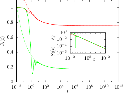
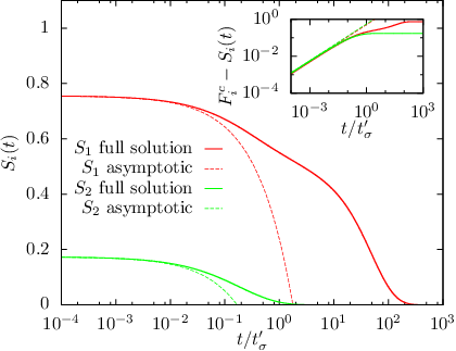
The $\alpha$- and $\beta$-relaxation processes are shown separately and in more detail in Fig. 3, including the asymptotic scaling laws derived in Ch. II.5.4. The $\beta$-relaxation of the critical correlator is depicted in the left panel. For $t>10^{2}$ there is no visible difference between the time fractal, $g(\hat{t})=\hat{t}^{-a}$, as derived in Eq. (47), and the correlator $S_{i}(t,\epsilon\rightarrow+0)$. Here, we emphasize that the emergent power-law exponent $a$ is a non-trivial result of the asymptotic expansion in a scenario with multiple decay channels presented in this manuscript. When approaching the critical point from below, a second relaxation process, called $\alpha$-relaxation, is observed (see right panel of Fig. 3). This decay from the plateau value $F_{i}^{\text{c}}$ is described by a second power law, $g(\hat{t})=-B\hat{t}^{b}$, which is commonly referred to as von Schweidler law Götze 2009. Interestingly, a distinct “kink” is observed in the $\alpha$-relaxation at $t/t_{\sigma}^{\prime}\approx 10$ that has not yet been reported for MCT dynamics. We will postpone its discussion to the next paragraph.

From the correlators discussed in the last paragraphs we also calculate the susceptibility spectra via Fourier transformation, relying on the modified Filon-Tuck algorithm Abramowitz and Stegun 1970; Tuck 1967. The results are presented in Fig. 4. As expected from the two-step relaxation scenario two distinct peaks are observed in the spectra for $\epsilon<0$. Both peaks are described using the critical spectra derived in the previous chapter (see Fig. 5). The figure shows that for several orders of magnitude in frequency a very good overlap between the asymptotic power laws and the numerical solution of the full MCT equations holds. All of these findings are in accordance to similar observations in bulk MCT Franosch et al. 1997. There is, however, one remarkable feature in the calculated susceptibility spectra, viz. the shoulder in the low-frequency peak in $\chi^{\prime\prime}_{1}(\omega)$, that is specific for our model and that corresponds to the observed “kink” in the correlation function. A similar feature has been identified as the Cole-Cole law in Ref. Sperl 2006, but in that case the “kink” emerges for frequencies larger than the von Schweidler law and thus cannot explain the shoulder observed in our model. The small-frequency susceptibility spectrum predicted by MCT with a single decay channel can be described by an asymmetric peak. (see also Fig. 4, right panel, since mode 2 has only one relaxation channel.) The right flank of this peak is given by the von Schweidler law and the left side corresponds to a Debye peak. The origin of the emergence of an additional shoulder therefore seems to be intrinsic for multiple decay channels: The correlator $S_{2}(t)$ decays slightly faster than $S_{1}(t)$ due to the smaller amplitude of $F_{2}^{\text{c}}$. We thus observe a faster relaxation of $\mathcal{M}^{\perp}_{1}(t)$ compared to $\mathcal{M}^{\parallel}_{1}(t)$ due to the asymmetry between $\delta^{\parallel}$ and $\delta^{\perp}$. Therefore, two overlapping peaks emerge in $\chi^{\prime\prime}_{1}(\omega)$, directly connected to those two decay channels. To support this explanation we have included the corresponding Debye peaks in Fig. 4, showing that the resulting spectrum, $\chi^{\prime\prime}_{1}(\omega)$, is indeed emerging from two distinct relaxation processes.

The observation of double peaks is an interesting finding in itself not directly connected to mode-coupling theory, but could also be observable in simulations or experiments for systems where multiple, very different decay channels come into play.

References

- Bengtzelius et al. (1984) Bengtzelius, U.; Götze, W.; Sjölander, A. Dynamics of supercooled liquids and the glass transition. Journal of Physics C: Solid State Physics 1984, 17, 5915–5934.
- Götze and Sjögren (1992) Götze, W.; Sjögren, L. Relaxation processes in supercooled liquids. Reports on Progress in Physics 1992, 55, 241–376.
- Götze (2009) Götze, W. Complex Dynamics of Glass-Forming Liquids - A Mode-Coupling Theory; Oxford University Press: Oxford, 2009.
- Götze (1987) Götze, W. Amorphous and Liquid Materials (pp. 34-81); Vol. 118 of NATO Advanced Study Institute, Series E: Applied Physics, edited by E. Lüscher, G. Fritsch, and G. Jacucci, 1987.
- Bosse and Thakur (1987) Bosse, J.; Thakur, J. S. Delocalization of small particles in a glassy matrix. Phys. Rev. Lett. 1987, 59, 998–1001.
- Barrat and Latz (1990) Barrat, J. L.; Latz, A. Mode coupling theory for the glass transition in a simple binary mixture. Journal of Physics: Condensed Matter 1990, 2, 4289–4295.
- Szamel and Löwen (1991) Szamel, G.; Löwen, H. Mode-coupling theory of the glass transition in colloidal systems. Phys. Rev. A 1991, 44, 8215–8219.
- Kob and Andersen (1995) Kob, W.; Andersen, H. C. Testing mode-coupling theory for a supercooled binary Lennard-Jones mixture I: The van Hove correlation function. Phys. Rev. E 1995, 51, 4626–4641.
- Voigtmann (2003) Voigtmann, Th. Dynamics of colloidal glass-forming mixtures. Phys. Rev. E 2003, 68, 051401.
- Franosch et al. (1997) Franosch, T.; Fuchs, M.; Götze, W.; Mayr, M. R.; Singh, A. P. Theory for the reorientational dynamics in glass-forming liquids. Phys. Rev. E 1997, 56, 5659–5674.
- Götze et al. (2000) Götze, W.; Singh, A. P.; Voigtmann, Th. Reorientational relaxation of a linear probe molecule in a simple glassy liquid. Phys. Rev. E 2000, 61, 6934–6949.
- Schilling and Scheidsteger (1997) Schilling, R.; Scheidsteger, T. Mode coupling approach to the ideal glass transition of molecular liquids: Linear molecules. Phys. Rev. E 1997, 56, 2932.
- Kämmerer et al. (1997) Kämmerer, S.; Kob, W.; Schilling, R. Dynamics of the rotational degrees of freedom in a supercooled liquid of diatomic molecules. Phys. Rev. E 1997, 56, 5450.
- Kämmerer et al. (1998) Kämmerer, S.; Kob, W.; Schilling, R. Test of mode coupling theory for a supercooled liquid of diatomic molecules. I. Translational degrees of freedom. Phys. Rev. E 1998, 58, 2131–2140.
- Kämmerer et al. (1998) Kämmerer, S.; Kob, W.; Schilling, R. Test of mode coupling theory for a supercooled liquid of diatomic molecules. II. -dependent orientational correlators. Phys. Rev. E 1998, 58, 2141–2150.
- Fabbian et al. (1999) Fabbian, L.; Latz, A.; Schilling, R.; Sciortino, F.; Tartaglia, P.; Theis, C. Molecular mode-coupling theory for supercooled liquids: Application to water. Phys. Rev. E 1999, 60, 5768–5777.
- Winkler et al. (2000) Winkler, A.; Latz, A.; Schilling, R.; Theis, C. Molecular mode-coupling theory applied to a liquid of diatomic molecules. Phys. Rev. E 2000, 62, 8004–8015.
- Chong and Hirata (1998) Chong, S.-H.; Hirata, F. Mode-coupling theory for molecular liquids based on the interaction-site model. Phys. Rev. E 1998, 58, 6188–6198.
- Chong et al. (2000) Chong, S.-H.; Götze, W.; Singh, A. P. Mode-coupling theory for the glassy dynamics of a diatomic probe molecule immersed in a simple liquid. Phys. Rev. E 2000, 63, 011206.
- Krakoviack (2005) Krakoviack, V. Liquid-Glass Transition of a Fluid Confined in a Disordered Porous Matrix: A Mode-Coupling Theory. Phys. Rev. Lett. 2005, 94, 065703.
- Krakoviack (2011) Krakoviack, V. Mode-coupling theory predictions for the dynamical transitions of partly pinned fluid systems. Phys. Rev. E 2011, 84, 050501.
- Lang et al. (2010) Lang, S.; Boţan, V.; Oettel, M.; Hajnal, D.; Franosch, T.; Schilling, R. Glass Transition in Confined Geometry. Phys. Rev. Lett. 2010, 105, 125701.
- Lang et al. (2012) Lang, S.; Schilling, R.; Krakoviack, V.; Franosch, T. Mode-coupling theory of the glass transition for confined fluids. Phys. Rev. E 2012, 86, 021502.
- Mandal et al. (2014) Mandal, S.; Lang, S.; Gross, M.; Oettel, M.; Raabe, D.; Franosch, T.; Varnik, F. Multiple reentrant glass transitions in confined hard-sphere glasses. Nature Communications 2014, 5, 4435.
- Mandal et al. (2017) Mandal, S.; Lang, S.; Boţan, V.; Franosch, T. Nonergodicity parameters of confined hard-sphere glasses. Soft Matter 2017, 13, 6167–6177.
- Fuchs and Cates (2002) Fuchs, M.; Cates, M. E. Theory of nonlinear rheology and yielding of dense colloidal suspensions. Phys. Rev. Lett. 2002, 89, 248304.
- Brader et al. (2007) Brader, J. M.; Voigtmann, Th.; Cates, M. E.; Fuchs, M. Dense colloidal suspensions under time-dependent shear. Phys. Rev. Lett. 2007, 98, 058301.
- Brader et al. (2009) Brader, J. M.; Voigtmann, Th.; Fuchs, M.; Larson, R. G.; Cates, M. E. Glass rheology: From mode-coupling theory to a dynamical yield criterion. Proceedings of the National Academy of Sciences 2009, 106, 15186–15191.
- Fuchs and Cates (2009) Fuchs, M.; Cates, M. E. A mode coupling theory for Brownian particles in homogeneous steady shear flow. Journal of Rheology 2009, 53, 957–1000.
- Kranz et al. (2010) Kranz, W. T.; Sperl, M.; Zippelius, A. Glass Transition for Driven Granular Fluids. Phys. Rev. Lett. 2010, 104, 225701.
- Kranz et al. (2013) Kranz, W. T.; Sperl, M.; Zippelius, A. Glass transition in driven granular fluids: A mode-coupling approach. Phys. Rev. E 2013, 87, 022207.
- Gazuz et al. (2009) Gazuz, I.; Puertas, A. M.; Voigtmann, Th.; Fuchs, M. Active and nonlinear microrheology in dense colloidal suspensions. Phys. Rev. Lett. 2009, 102, 248302.
- Gruber et al. (2016) Gruber, M.; Abade, G. C.; Puertas, A. M.; Fuchs, M. Active microrheology in a colloidal glass. Phys. Rev. E 2016, 94, 042602.
- Gruber (2019) Gruber, M. Theory of microrheology in complex fluids. PhD thesis, Universität Konstanz; 2019; http://nbn-resolving.de/urn:nbn:de:bsz:352-2-hurftyctohii2.
- Şenbil et al. (2019) Şenbil, N.; Gruber, M.; Zhang, C.; Fuchs, M.; Scheffold, F. Observation of strongly heterogeneous dynamics at the depinning transition in a colloidal glass. Phys. Rev. Lett. 2019, 122, 108002.
- Nandi and Gov (2017) Nandi, S. K.; Gov, N. S. Nonequilibrium mode-coupling theory for dense active systems of self-propelled particles. Soft Matter 2017, 13, 7609–7616.
- Liluashvili et al. (2017) Liluashvili, A.; Ónody, J.; Voigtmann, Th. Mode-coupling theory for active Brownian particles. Phys. Rev. E 2017, 96, 062608.
- Janssen (2019) Janssen, L. M. C. Active glasses. Journal of Physics: Condensed Matter 2019, 31, 503002.
- Götze (1990) Götze, W. The scaling functions for the -relaxation process of supercooled liquids and glasses. Journal of Physics: Condensed Matter 1990, 2, 8485–8498.
- Franosch et al. (1997) Franosch, T.; Fuchs, M.; Götze, W.; Mayr, M. R.; Singh, A. P. Asymptotic laws and preasymptotic correction formulas for the relaxation near glass-transition singularities. Phys. Rev. E 1997, 55, 7153–7176.
- Elizondo-Aguilera and Voigtmann (2019) Elizondo-Aguilera, L. F.; Voigtmann, Th. Glass-transition asymptotics in two theories of glassy dynamics: Self-consistent generalized Langevin equation and mode-coupling theory. Phys. Rev. E 2019, 100, 042601.
- Szamel (2003) Szamel, G. Colloidal Glass Transition: Beyond Mode-Coupling Theory. Phys. Rev. Lett. 2003, 90, 228301.
- Janssen (2018) Janssen, L. M. C. Mode-Coupling Theory of the Glass Transition: A Primer. Frontiers in Physics 2018, 6, 97.
- Luo and Janssen (2019) Luo, C.; Janssen, L. M. C. Generalized mode-coupling theory of the glass transition. I. Numerical results for Percus-Yevick hard spheres. arXiv:1909.00428 2019,
- van Megen and Underwood (1993) van Megen, W.; Underwood, S. M. Glass transition in colloidal hard spheres: Mode-coupling theory analysis. Phys. Rev. Lett. 1993, 70, 2766–2769.
- van Megen and Underwood (1994) van Megen, W.; Underwood, S. M. Glass transition in colloidal hard spheres: Measurement and mode-coupling-theory analysis of the coherent intermediate scattering function. Phys. Rev. E 1994, 49, 4206–4220.
- Li et al. (1992) Li, G.; Du, W.; Chen, X.; Cummins, H.; Tao, N. Testing mode-coupling predictions for and relaxation in near the liquid-glass transition by light scattering. Phys. Rev. A 1992, 45, 3867.
- Li et al. (1992) Li, G.; Du, W.; Sakai, A.; Cummins, H. Light-scattering investigation of and relaxation near the liquid-glass transition of the molecular glass salol. Phys. Rev. A 1992, 46, 3343.
- Singh et al. (1998) Singh, A.; Li, G.; Götze, W.; Fuchs, M.; Franosch, T.; Cummins, H. Structural relaxation in orthoterphenyl: a schematic mode-coupling-theory model analysis. Journal of Non-Crystalline Solids 1998, 235-237, 66 – 70.
- Lunkenheimer et al. (1996) Lunkenheimer, P.; Pimenov, A.; Dressel, M.; Goncharov, Y. G.; Böhmer, R.; Loidl, A. Fast Dynamics of Glass-Forming Glycerol Studied by Dielectric Spectroscopy. Phys. Rev. Lett. 1996, 77, 318–321.
- Schneider et al. (1999) Schneider, U.; Lunkenheimer, P.; Brand, R.; Loidl, A. Broadband dielectric spectroscopy on glass-forming propylene carbonate. Phys. Rev. E 1999, 59, 6924–6936.
- Götze and Voigtmann (2000) Götze, W.; Voigtmann, Th. Universal and nonuniversal features of glassy relaxation in propylene carbonate. Phys. Rev. E 2000, 61, 4133.
- Kob and Andersen (1994) Kob, W.; Andersen, H. C. Scaling Behavior in the -Relaxation Regime of a Supercooled Lennard-Jones Mixture. Phys. Rev. Lett. 1994, 73, 1376–1379.
- Das et al. (2008) Das, S. K.; Horbach, J.; Voigtmann, Th. Structural relaxation in a binary metallic melt: Molecular dynamics computer simulation of undercooled . Phys. Rev. B 2008, 78, 064208.
- Gallo et al. (1996) Gallo, P.; Sciortino, F.; Tartaglia, P.; Chen, S.-H. Slow dynamics of water molecules in supercooled states. Phys. Rev. Lett. 1996, 76, 2730.
- Sciortino et al. (1996) Sciortino, F.; Gallo, P.; Tartaglia, P.; Chen, S. H. Supercooled water and the kinetic glass transition. Phys. Rev. E 1996, 54, 6331–6343.
- Sciortino et al. (1997) Sciortino, F.; Fabbian, L.; Chen, S.-H.; Tartaglia, P. Supercooled water and the kinetic glass transition. II. Collective dynamics. Phys. Rev. E 1997, 56, 5397.
- Sciortino and Kob (2001) Sciortino, F.; Kob, W. Debye-Waller Factor of Liquid Silica: Theory and Simulation. Phys. Rev. Lett. 2001, 86, 648–651.
- Horbach et al. (1998) Horbach, J.; Kob, W.; Binder, K. Molecular dynamics simulation of the dynamics of supercooled silica. Philosophical Magazine B 1998, 77, 297–303.
- Voigtmann and Horbach (2006) Voigtmann, Th.; Horbach, J. Slow dynamics in ion-conducting sodium silicate melts: Simulation and mode-coupling theory. Europhys. Lett. 2006, 74, 459–465.
- (61) See Ref. [(10)] and A. P. Singh, PhD thesis, Technische Universität München; 1998.
- Rinaldi et al. (2001) Rinaldi, A.; Sciortino, F.; Tartaglia, P. Dynamics in a supercooled molecular liquid: Theory and simulations. Phys. Rev. E 2001, 63, 061210.
- Krieger and Bosse (1987) Krieger, U.; Bosse, J. relaxation of a simple molten salt near the glass transition. Phys. Rev. Lett. 1987, 59, 1601–1604.
- Lang et al. (2013) Lang, S.; Schilling, R.; Franosch, T. Mode-coupling theory for multiple decay channels. Journal of Statistical Mechanics: Theory and Experiment 2013, 2013, P12007.
- Zwanzig (2001) Zwanzig, R. Nonequilibrium statistical mechanics; Oxford University Press, 2001.
- Hansen and McDonald (2006) Hansen, J. P.; McDonald, I. R. Theory of Simple Liquids; Academic Press, 2006.
- Franosch (2014) Franosch, T. Long-time limit of correlation functions. Journal of Physics A: Mathematical and Theoretical 2014, 47, 325004.
- Franosch and Voigtmann (2002) Franosch, T.; Voigtmann, Th. Completely Monotone Solutions of the Mode-Coupling Theory for Mixtures. J. Stat. Phys. 2002, 109, 237–259.
- Sentjabrskaja et al. (2016) Sentjabrskaja, T.; Zaccarelli, E.; De Michele, C.; Sciortino, F.; Tartaglia, P.; Voigtmann, Th.; Egelhaaf, S. U.; Laurati, M. Anomalous dynamics of intruders in a crowded environment of mobile obstacles. Nature Communications 2016, 7, 11133.
- (70) For detailed discussions of the bifurcation scenario and its consequences we refer the reader to Ref. (40) () and Ref. (71) ().
- Götze and Sperl (2002) Götze, W.; Sperl, M. Logarithmic relaxation in glass-forming systems. Phys. Rev. E 2002, 66, 011405.
- Sperl (2000) Sperl, M. Glass Transition in Colloids with Attractive Interaction. Diploma thesis, Technische Universität München; 2000.
- Abramowitz and Stegun (1970) Abramowitz, M.; Stegun, I. A. Handbook of Mathematical Functions; Dover Publications, New York, 1970.
- Tuck (1967) Tuck, E. O. A Simple ”Filon-Trapezoidal” Rule. Mathematics of Computation 1967, 21, 239.
- Sperl (2006) Sperl, M. Cole-Cole law for critical dynamics in glass-forming liquids. Phys. Rev. E 2006, 74, 011503.
- Mandal et al. (2019) Mandal, S.; Schrack, L.; Löwen, H.; Sperl, M.; Franosch, T. Persistent Anti-Correlations in Brownian Dynamics Simulations of Dense Colloidal Suspensions Revealed by Noise Suppression. Phys. Rev. Lett. 2019, 123, 168001.
achemso-control