跳到论文正文
W Papers独立论文阅读器 arXiv:2005.13097 论文正文 计算阅读时间 · 0%
引用这篇论文根据当前论文元数据生成,正式投稿前建议核对。


License: arXiv.org perpetual non-exclusive license
arXiv:2005.13097v1 [stat.ML] 27 May 2020

On the Convergence of Langevin Monte Carlo:
The Interplay between Tail Growth and Smoothness

Murat A. Erdogdu Thanks:  Department of Computer Science and Department of Statistical Sciences at the University of Toronto, and Vector Institute    Rasa Hosseinzadeh Thanks:  Department of Computer Science at the University of Toronto, and Vector Institute
Abstract

We study sampling from a target distribution ν∗=e−f{\nu_{*}=e^{-f}} using the unadjusted Langevin Monte Carlo (LMC) algorithm. For any potential function ff whose tails behave like ‖x‖α{\|x\|^{\alpha}} for α∈[1,2]{\alpha\in[1,2]}, and has β\beta-Hölder continuous gradient, we prove that 𝒪~(d1β+1+ββ(2α−𝟙{α≠1})ϵ−1β){\widetilde{\mathcal{O}}\raisebox{2.15277pt}{\big(}d^{\frac{1}{\beta}+\frac{1+\beta}{\beta}(\frac{2}{\alpha}-{\mathbbm{1}}_{\{\alpha\neq 1\}})}\epsilon^{-\frac{1}{\beta}}\raisebox{2.15277pt}{\big)}} steps are sufficient to reach the ϵ\epsilon-neighborhood of a dd-dimensional target distribution ν∗\nu_{*} in KL-divergence. This convergence rate, in terms of ϵ\epsilon dependency, is not directly influenced by the tail growth rate α\alpha of the potential function as long as its growth is at least linear, and it only relies on the order of smoothness β\beta. One notable consequence of this result is that for potentials with Lipschitz gradient, i.e. β=1\beta=1, the above rate recovers the best known rate 𝒪~​(d​ϵ−1){\widetilde{\mathcal{O}}(d\epsilon^{-1})} which was established for strongly convex potentials in terms of ϵ\epsilon dependency, but we show that the same rate is achievable for a wider class of potentials that are degenerately convex at infinity. The growth rate α\alpha starts to have an effect on the established rate in high dimensions where dd is large; furthermore, it recovers the best-known dimension dependency when the tail growth of the potential is quadratic, i.e. α=2{\alpha=2}, in the current setup.

We establish the convergence rate of LMC by first proving a moment dependent modified log-Sobolev inequality with explicit constants for a class of target distributions that have convex degenerate potentials at infinity. Then, we prove linearly diverging estimates for any order moments of the Markov chain defined by the LMC algorithm, and show that this is sufficient to obtain the above convergence rate. Our framework also allows for finite perturbations, and any order of smoothness β∈(0,1]{\beta\in(0,1]}; consequently, our results are applicable to a wide class of non-convex potentials that are weakly smooth and exhibit at least linear tail growth.

1 Introduction

Sampling from a target distribution using Markov chain Monte Carlo (MCMC) is a fundamental problem in statistics, and it often amounts to discretizing a continuous-time diffusion process with invariant measure as the target. When the target distribution corresponds to the Gibbs measure ν∗=e−f{\nu_{*}=e^{-f}} where f:ℝd→ℝ{f:\mathbb{R}^{d}\to\mathbb{R}} is the potential function satisfying ∫e−f⁡(x)​𝑑x=1{\int e^{-f(x)}dx=1}, a popular candidate diffusion is the overdamped Langevin diffusion, which is the solution of the following stochastic differential equation (SDE),

d​Zt=−∇f​(Zt)​d​t+2​d​Bt,dZ_{t}=-\nabla f(Z_{t})dt+\sqrt{2}dB_{t}, (1.1)

where BtB_{t} is a dd-dimensional Brownian motion. It is straightforward to show that the Langevin diffusion (1.1) admits the target Gibbs measure ν∗\nu_{*} as its invariant distribution [MCF15]. In general, simulating a continuous-time diffusion such as (1.1) is impractical; thus, a numerical integration scheme is needed to approximate it. Due to its simplicity, efficiency, and well-understood theoretical properties, algorithms based on Langevin diffusion have found numerous applications in sampling and optimization literature [WT11, Dal17a, RRT17, XCZG18, LWME19]. In this work, we focus on the unadjusted Langevin Monte Carlo algorithm (LMC) which is the Euler discretization of the overdamped Langevin diffusion (1.1) and relies on the following update rule

xk+1=xk−η∇f(xk)+2​ηWk,x_{k+1}=x_{k}-\eta\nabla f(x_{k})+\sqrt{2\eta}W_{k}, (1.2)

where WkW_{k} is an isotropic Gaussian vector independent from WmW_{m} and xmx_{m} for m<km<k, and η\eta is the step size. LMC defines a Markov chain which has an invariant measure that is different than the target ν∗\nu_{*}, and this difference is often termed as the bias which is due to the numerical integration. The bias of a discretized diffusion such as LMC can be generally controlled with a smaller step size, where in the limit case η↓0{\eta\downarrow 0}, the iteration (1.2) scaled with 1/η{1/\eta} reduces to the SDE (1.1).

Convergence rate of LMC has been the focus of recent research. Rates are established under structural assumptions on the potential function, and they quantify the number of iterations required to reach the ϵ\epsilon-neighborhood of a dd-dimensional target distribution ν∗=e−f\nu_{*}=e^{-f} under a particular distance measure – our focus is on KL-divergence. Earlier attempts established convergence rates under the global curvature assumptions on the potential function. For example, for strongly convex and smooth potentials, the convergence rate of 𝒪~​(d​ϵ−1){\widetilde{\mathcal{O}}(d\epsilon^{-1})} has been shown [Dal17b], whereby smooth function is a function with Lipschitz continuous gradient. We note that higher-order smoothness on the potential function may improve the convergence rate [MFWB19b]; however, we consider only the first-order smoothness in the current paper. For convex and smooth potentials with growth rate α\alpha, a convergence rate of 𝒪~​(d1+4/α​ϵ−3){\widetilde{\mathcal{O}}(d^{1+4/\alpha}\epsilon^{-3})} is known to hold for LMC [CB18]. More recently, however, it has been observed that tail growth structure is the determinant factor in sampling [CCAY+18, Ebe16, EMS18, EGZ19], rather than the global curvature structure such as (strong) convexity, where in this context, a strongly convex potential is understood to exhibit quadratic growth. Growth-based structural conditions has the additional benefit of allowing for finite perturbations, which in turn allows for sampling from non-convex potentials with a wide range of modern applications in statistics. A condition on the target distribution ν∗\nu_{*} that fits in this framework is the log-Sobolev inequality (LSI) of Bakry and Emery [BE85], which can be written as

∀ρ,H​(ρ|ν∗)≤λ​I​(ρ|ν∗),\displaystyle\forall\rho,\ \ \textnormal{H}\big({\rho}|{\nu_{*}}\big)\leq\lambda\textnormal{I}\big({\rho}|{\nu_{*}}\big), (1.3)

where H​(ρ|ν∗)\textnormal{H}\big({\rho}|{\nu_{*}}\big) denotes the KL-divergence (relative entropy) and I​(ρ|ν∗)\textnormal{I}\big({\rho}|{\nu_{*}}\big) denotes the relative Fisher information between ρ\rho and ν∗\nu_{*}, and λ>0{\lambda>0} is the log-Sobolev constant. The LSI condition (1.3) can be verified for potentials with certain growth structure. Indeed, it is known to hold for strongly convex potentials [BE85], and it allows for finite perturbations due to Holley-Stroock perturbation lemma [HS87]; thus, potentials that have quadratic growth can be shown to satisfy LSI (this will be made precise later). Denoting the distribution of Langevin diffusion (1.1) at time tt with ρt\rho_{t}, it is known that dd​t​H​(ρt|ν∗)=−I​(ρt|ν∗){\tfrac{d}{dt}\textnormal{H}\big({\rho_{t}}|{\nu_{*}}\big)=-\textnormal{I}\big({\rho_{t}}|{\nu_{*}}\big)} which, combined with the LSI condition (1.3) entails a differential inequality of the form dd​t​H​(ρt|ν∗)≤−1λ​H​(ρt|ν∗){\frac{d}{dt}\textnormal{H}\big({\rho_{t}}|{\nu_{*}}\big)\leq-\frac{1}{\lambda}\textnormal{H}\big({\rho_{t}}|{\nu_{*}}\big)}, which in turn yields an exponential contraction in KL-divergence, i.e., H(ρt|ν∗)≤e−t/λH(ρ0|ν∗){\textnormal{H}\big({\rho_{t}}|{\nu_{*}}\big)\leq e^{-t/\lambda}\textnormal{H}\big({\rho_{0}}|{\nu_{*}}\big)} for the diffusion process.

An important implication of a condition like LSI (1.3) in the context of sampling with LMC is that fast mixing properties of the continuous-time diffusion induced by LSI are inherited by the discrete algorithm LMC. That is, LSI coupled with the smoothness condition on the potential is sufficient to obtain the fast convergence rate 𝒪~​(d​ϵ−1){\widetilde{\mathcal{O}}(d\epsilon^{-1})} [VW19], which is the best known rate for LMC in this framework. The significance of this result is in that, it relaxes the strong convexity assumption which is a global curvature condition on ff to the LSI condition (1.3), which can be regarded as a tail growth condition on ff, allowing for perturbations and consequently sampling from non-convex potentials.

The fundamental idea leading to the current paper is that the fast convergence of LMC does not require an exponentially contracting Langevin diffusion, which is essentially obtained under strong tail growth conditions on the potential. A representative convergence analysis of the LMC algorithm under some distance measure D (our main focus is KL-divergence) starts with establishing a single step bound in the following sense,

∀k∈ℕ,D​(ρk+1|ν∗)≤r⁡(η)​D​(ρk|ν∗)+C​ηθ,\displaystyle\forall k\in\mathbb{N},\ \ \textnormal{D}(\rho_{k+1}|\nu_{*})\leq r(\eta)\,\textnormal{D}(\rho_{k}|\nu_{*})+C\eta^{\theta}, (1.4)

where r:[0,∞)→[0,1]{r:[0,\infty)\to[0,1]} is a monotone decreasing function which is typically inherited from the fast decaying diffusion counterpart. The discretization error C​ηθ{C\eta^{\theta}} can be made small with smaller step size η\eta, and the exponent θ\theta is intrinsic to the numerical scheme as well as the order of smoothness of the potential. Elementary algebra reveals that, one can iterate the inequality (1.4) and achieve convergence as long as r⁡(η)<1{r(\eta)<1}. Recent literature focused on exponential decays rexp​(t)=e−α​t{r_{\exp}(t)=e^{-\alpha t}} which are usually established under conditions like LSI (1.3) or strong convexity that correspond to potentials exhibiting quadratic growth (see, for example [Dal17b, VW19]). Nevertheless, the inequality (1.4) by no means benefits from the exponential decay, as r⁡(t)r(t) is only evaluated at short time horizons t=η{t=\eta}. Indeed, any decreasing rate function r⁡(t)r(t) satisfying r⁡(0)=1{r(0)=1} and r′​(0)<0{r^{\prime}(0)<0} would achieve the same rate of convergence as exponential decay rexp​(t){r_{\text{exp}}(t)}. For example, consider the algebraic rate ralg​(t)=1/(1+α​t){r_{\text{alg}}(t)=1/(1+\alpha t)} which is much slower than the exponential rate, but it provides the same level of decay in small time horizons, i.e. evaluated at the step size η\eta, one has

ralg​(η)≈rexp​(η)≈1−α​η​ when η is small.\displaystyle r_{\text{alg}}(\eta)\approx r_{\exp}(\eta)\approx 1-\alpha\eta\ \text{ when $\eta$ is small.} (1.5)

However, in contrast to exponential decay, algebraic rates can be obtained under much weaker tail growth conditions on the potential function ff.

Modified versions of the LSI condition (1.3) or weak Poincaré inequalities are commonly employed in the analysis of diffusion processes [BGL13], and can be used to explain different convergence behavior. For example in the seminal work by [TV00], a modified log-Sobolev inequality is used to establish a convergence rate of 𝒪⁡(t−κ){\mathcal{O}(t^{-\kappa})} for all κ>0{\kappa>0} for the Langevin diffusion (1.1) (𝒪⁡(t−∞)\mathcal{O}(t^{-\infty}) in their notation). Our results build on a similar construction. For a class of potentials that are convex degenerate at infinity, with tails growing like ‖x‖α{\|x\|^{\alpha}} for α∈[1,2]{\alpha\in[1,2]}, we establish the following modified log-Sobolev inequality (mLSI)

∀ρ,\displaystyle\forall\rho,\ \ H​(ρ|ν∗)≤λ​I​(ρ|ν∗)1−δ​Ms​(ρ+ν∗)δ with δ∈[0,1/2),\displaystyle\textnormal{H}\big({\rho}|{\nu_{*}}\big)\leq\lambda\textnormal{I}\big({\rho}|{\nu_{*}}\big)^{1-\delta}\textnormal{M}_{s}(\rho+\nu_{*})^{\delta}\ \ \text{ with }\ \ \delta\in[0,1/2), (1.6)

where Ms​(ρ)=∫(1+‖x‖2)s/2​ρ​(x)​𝑑x{\textnormal{M}_{s}(\rho)=\int(1+\|x\|^{2})^{s/2}\rho(x)dx} is the ss-th moment of any function ρ\rho. This inequality entails a decay with the desired properties (1.5) under mild conditions on the potential. By further assuming that the gradient of the potential is β\beta-Hölder continuous and carefully tuning the moment order s=𝒪⁡(log⁡(d/ϵ)){s=\mathcal{O}(\log(d/\epsilon))} in mLSI (1.6), we can prove that, even with linearly diverging moment estimates for the LMC iterates, the algorithm is guaranteed to reach the ϵ\epsilon-neighborhood of a dd-dimensional target ν∗\nu_{*} in KL-divergence after taking the advertised number of steps N=𝒪~(d1β+1+ββ(2α−𝟙{α≠1})ϵ−1β){N=\widetilde{\mathcal{O}}\raisebox{2.15277pt}{\big(}d^{\frac{1}{\beta}+\frac{1+\beta}{\beta}(\frac{2}{\alpha}-{\mathbbm{1}}_{\{\alpha\neq 1\}})}\epsilon^{-\frac{1}{\beta}}\raisebox{2.15277pt}{\big)}}. In moderate dimensions d≪ϵ−1{d\ll\epsilon^{-1}}, this convergence rate does not depend on the tail growth rate α\alpha, and it is controlled solely by the order of smoothness β\beta, whereas in high dimensions d=𝒪⁡(ϵ−1){d=\mathcal{O}(\epsilon^{-1})}, the rate is determined by an interplay between the growth rate and the order of smoothness. The above rate also recovers the best known rate which was established for smooth potentials (β=1{\beta=1}) under the LSI condition (1.3) where the tail growth is quadratic (α=2)(\alpha=2).

Our contributions can be summarized as follows.

  • •

    For a potential function ff whose tails behave like ‖x‖α{\|x\|^{\alpha}}, and has β\beta-Hölder continuous gradient, i.e.,

    f⁡(x)∼‖x‖α​ for ​α∈[1,2], and ‖∇f​(x)−∇f​(y)‖≤L​‖x−y‖β∀x,y,\displaystyle f(x)\sim\|x\|^{\alpha}\ \text{ for }\ \alpha\in[1,2],\ \ \text{ and }\ \ \|\nabla f(x)-\nabla f(y)\|\leq L\|x-y\|^{\beta}\ \ \ \forall x,y, (1.7)

    we prove that LMC achieves the convergence rate 𝒪~(d1β+1+ββ(2α−𝟙{α≠1})ϵ−1β){\widetilde{\mathcal{O}}\raisebox{2.15277pt}{\big(}d^{\frac{1}{\beta}+\frac{1+\beta}{\beta}(\frac{2}{\alpha}-{\mathbbm{1}}_{\{\alpha\neq 1\}})}\epsilon^{-\frac{1}{\beta}}\raisebox{2.15277pt}{\big)}} in KL-divergence. In moderate dimensions when d≪ϵ−1{d\ll\epsilon^{-1}}, the tail growth rate α\alpha does not impact the convergence rate, whereas in high dimensions where d=𝒪⁡(ϵ−1){d=\mathcal{O}(\epsilon^{-1})}, tail growth enters the convergence rate through dimension dependency.

  • •

    As a key step in deriving the above convergence rate, we establish a modified log-Sobolev inequality (mLSI) (1.6) with explicit constant λ\lambda, and a target dependent moment function Ms​(ρ+ν∗){\textnormal{M}_{s}(\rho+\nu_{*})} for any order s≥2s\geq 2. Both of these are crucial in deriving a convergence rate with correct dependence on the dimension dd as well as the accuracy ϵ\epsilon. The final convergence result is obtained by employing the mLSI condition (1.6) for the optimal moment order s=𝒪⁡(log⁡(d/ϵ)){s=\mathcal{O}(\log(d/\epsilon))}.

  • •

    In lieu of (1.7), we are mainly interested in potentials exhibiting weak dissipativity, i.e.,

    ⟨x,∇f​(x)⟩≥a​∥x∥α−b with α∈[1,2),a,b>0.\displaystyle{\langle x,\nabla f(x)\rangle}\geq a\lVert x\rVert^{\alpha}-b\ \ \text{ with }\ \ \alpha\in[1,2),\ \ a,b>0. (1.8)

    In order to use the condition mLSI (1.6), we establish linearly diverging moment estimates for the LMC iterates under (1.8). Somewhat surprisingly, this is sufficient to establish the convergence of LMC in KL-divergence.

  • •

    Our convergence results are valid under finite perturbations of the potential; consequently, they cover sampling from non-convex potentials with at least linear growth. Furthermore, our results also cover the case β<1{\beta<1} for which the potential function is not smooth; more specifically, it does not have a Lipschitz gradient. To the best of our knowledge, this is the first convergence result for the LMC algorithm for weakly smooth potentials that exhibit subquadratic growth, which does not rely on regularization or Gaussian smoothing.

  • •

    Finally, using Csiszár-Kullback-Pinsker inequalities, the above convergence rates obtained under KL-divergence can be translated to estimates in total variation and LαL_{\alpha}-Wasserstein metrics with respective rates 𝒪~(d1β+1+ββ(2α−𝟙{α≠1})ϵ−2β){\widetilde{\mathcal{O}}\raisebox{2.15277pt}{\big(}d^{\frac{1}{\beta}+\frac{1+\beta}{\beta}(\frac{2}{\alpha}-{\mathbbm{1}}_{\{\alpha\neq 1\}})}\epsilon^{-\frac{2}{\beta}}\raisebox{2.15277pt}{\big)}} and 𝒪~(d3β+1+ββ(2α−𝟙{α≠1})ϵ−2​αβ){\widetilde{\mathcal{O}}\raisebox{2.15277pt}{\big(}d^{\frac{3}{\beta}+\frac{1+\beta}{\beta}(\frac{2}{\alpha}-{\mathbbm{1}}_{\{\alpha\neq 1\}})}\epsilon^{-\frac{2\alpha}{\beta}}\raisebox{2.15277pt}{\big)}}.

Rest of the paper is organized as follows. Section 1.1 reviews our notation, and Section 2 surveys the related work with a detailed comparison on the existing convergence rates. In Section 3, we establish the main technical results on the convergence of LMC for potentials with certain growth and smoothness properties. Section 4 discusses further implications of the tools developed in Section 3. We give concrete examples in Section 5, by applying these tools to non-convex sampling problems that are also weakly smooth. Proofs of the main theorems and corollaries are provided in Sections 6, 7, 8, 9 and 10 in order of appearance of their statement in the main text. Finally, we conclude in Section 11 with brief remarks on future work.

1.1 Notation

For a real number x∈ℝ{x\in\mathbb{R}}, we denote its absolute value with |x|\mathopen{}\mathclose{{\left|x}}\right|. We denote the pp-norm of a vector x∈ℝd{x\in\mathbb{R}^{d}} with ∥x∥p\lVert x\rVert_{p} and whenever p=2{p=2}, we omit the subscript and simply write ‖x‖≜‖x‖2{\|x\|\triangleq\|x\|_{2}} to ease the notation. For a matrix A∈ℝd×k{A\in\mathbb{R}^{d\times k}}, Ai​jA_{ij} denotes its entry in the ii-th row and jj-th column, and whenever d=k{d=k}, its trace is denoted by Tr⁡(A)=Σi=1d​Ai​i{\Tr(A)=\Sigma_{i=1}^{d}A_{ii}}. We use Id{I}_{d} to denote the identity matrix in dd-dimensions.

For a function f:ℝd→ℝ{f:\mathbb{R}^{d}\to\mathbb{R}}, we define its infinity norm as ‖f‖∞=supx∈ℝd|f⁡(x)|{\|f\|_{\infty}=\sup_{x\in\mathbb{R}^{d}}|f(x)|}. Ms​(f){\textnormal{M}_{s}(f)} is used to denote the modified ss-th moment of the function ff (which is not necessarily a distribution), defined as Ms​(f)=∫f⁡(x)​(1+‖x‖2)s/2​𝑑x{\textnormal{M}_{s}(f)=\int f(x)(1+\|x\|^{2})^{s/2}dx}. The gradient and the Hessian of ff are denoted by ∇f​(x){\nabla f(x)} and ∇2f​(x){\nabla^{2}f(x)}, respectively, where the derivatives are with respect to xx. For a statement AA, the indicator function is denoted with 𝟙{A}{\mathbbm{1}}_{\{A\}} and defined as

𝟙{A}={1if A is true,0otherwise.\displaystyle{\mathbbm{1}}_{\{A\}}=\mathopen{}\mathclose{{\left\{\begin{array}[]{ll}1&\text{if $A$ is true,}\\ 0&\text{otherwise.}\\ \end{array}}}\right.

We use 𝔼[x]\mathbb{E}\mathopen{}\mathclose{{\left[x}}\right] to denote the expected value of a random variable xx, where expectations are over all the randomness inside the brackets. For probability densities pp,qq on ℝd\mathbb{R}^{d}, we use H​(p|q)\textnormal{H}\big({p}|{q}\big) and I​(p|q)\textnormal{I}\big({p}|{q}\big) to denote their KL-divergence (or relative entropy) and relative Fisher information, respectively, which are defined as

H​(p|q)=∫p⁡(x)​log⁡p⁡(x)q⁡(x)​𝑑x, and I​(p|q)=∫p⁡(x)​‖∇log⁡p⁡(x)q⁡(x)‖2​𝑑x.\displaystyle\textnormal{H}\big({p}|{q}\big)=\int p(x)\log{\frac{p(x)}{q(x)}}dx,\ \ \ \text{ and }\ \ \ \textnormal{I}\big({p}|{q}\big)=\int p(x)\Big\|\nabla\log{\frac{p(x)}{q(x)}}\Big\|^{2}dx.

Similarly, we denote the entropy of pp with H(pCLOSE)=−∫p(x)logp(x)dx{\textnormal{H}\mathopen{}\mathclose{{\left({p}}}\right)=-\int p(x)\log{p(x)}dx}. Denoting the Borel σ\sigma-field of ℝd\mathbb{R}^{d} with ℬ⁡(ℝd){\mathcal{B}(\mathbb{R}^{d})}, LαL_{\alpha}-Wasserstein for α>0{\alpha>0} and total variation metrics are defined as

OPEN𝒲α​(p,q)=infν(∫∥x−y∥α​𝑑ν​(p,q)CLOSE)1/α,\displaystyle\mathcal{W}_{\alpha}(p,q)=\inf_{\nu}\mathopen{}\mathclose{{\left(\int\lVert x-y\rVert^{\alpha}d\nu(p,q)}}\right)^{{1}/{\alpha}}, TV(p,qCLOSE)=supA∈ℬ⁡(ℝd)|∫Ap(x)dx−∫Aq(x)dx|,\displaystyle\mathrm{TV}\mathopen{}\mathclose{{\left(p,q}}\right)=\sup_{A\in\mathcal{B}(\mathbb{R}^{d})}\mathopen{}\mathclose{{\left|\int_{A}p(x)dx-\int_{A}q(x)dx}}\right|,

where in the first formula, infimum runs over the set of probability measures on ℝd×ℝd{\mathbb{R}^{d}\times\mathbb{R}^{d}} that has marginals with corresponding densities pp and qq.

Finally, 𝒪\mathcal{O} and 𝒪~\widetilde{\mathcal{O}} notations are frequently used to describe the dependence of a function ff on another function gg, and defined in the following sense

f⁡(x)=𝒪⁡(g⁡(x))⟹lim supx→∞f⁡(x)g⁡(x)<∞, and ​f​(x)=𝒪~​(g⁡(x))⟹lim supx→∞f⁡(x)g⁡(x)​log⁡(g⁡(x))k<∞,\displaystyle f(x)=\mathcal{O}(g(x))\implies\limsup_{x\to\infty}\frac{f(x)}{g(x)}<\infty,\ \text{ and }\ f(x)=\widetilde{\mathcal{O}}(g(x))\implies\limsup_{x\to\infty}\frac{f(x)}{g(x)\log(g(x))^{k}}<\infty,

for some k≥0k\geq 0, where 𝒪~\widetilde{\mathcal{O}} simply ignores the logarithmic factors. We use f⁡(x)≲g⁡(x)f(x)\lesssim g(x) instead of f⁡(x)≤𝒪⁡(g⁡(x))f(x)\leq\mathcal{O}(g(x)) to improve readability.

2 Related Work

The LMC algorithm has been extensively studied in the context of sampling from a log-concave target distribution. Earlier results focused on characterizing its bias which is also referred to as the integration error [Mil94, MT13], and the convergence guarantees were mostly asymptotic [GM91, MT12]. Non-asymptotic analysis of LMC has drawn a lot of interest recently [DT12, Dal17a, Dal17b, DMM19, CB18, CCAY+18, VW19, DK19, BDMS19] where the focus was on potentials exhibiting strong tail growth properties. These papers were mostly influenced by the pioneering works by Dalalyan [Dal17b], and Durmus and Moulines [DM16, DM17] where it was shown that for strongly convex and smooth potentials, LMC reaches ϵ\epsilon accuracy in terms of total variation (TV) distance after 𝒪~​(d​ϵ−2)\widetilde{\mathcal{O}}(d\epsilon^{-2}) steps. Similarly, OPEN𝒪~​(d​ϵ−2CLOSE){\widetilde{\mathcal{O}}\mathopen{}\mathclose{{\left(d\epsilon^{-2}}}\right)} steps are sufficient to reach ϵ\epsilon accuracy under the L2L_{2}-Wasserstein distance [DM19], which can be further improved to OPEN𝒪~​(d​ϵ−1CLOSE){\widetilde{\mathcal{O}}\mathopen{}\mathclose{{\left(d\epsilon^{-1}}}\right)} under an additional second-order smoothness assumption on the potential function.

In this paper, we establish guarantees under KL-divergence (relative entropy) which can be easily translated to TV and Wasserstein metrics using Csiszár-Kullback-Pinsker (CKP) [BV05] and/or Talagrand inequalities [Tal96, OV00]. For strongly convex and smooth potentials, it is known that OPEN𝒪~​(d​ϵ−1CLOSE){\widetilde{\mathcal{O}}\mathopen{}\mathclose{{\left(d\epsilon^{-1}}}\right)} steps of LMC yield an ϵ\epsilon accurate sample in KL-divergence [CB18, DMM19]. This is still the best known rate in this setup, and recovers the best known rates in TV [DM17, Dal17b] as well as in L2L_{2}-Wasserstein metrics [DM19]. However, for convex and smooth potentials that grow like ‖x‖α\|x\|^{\alpha}, the rate drops to 𝒪~​(d1+4α​ϵ−3){\widetilde{\mathcal{O}}\big(d^{1+\frac{4}{\alpha}}\epsilon^{-3}\big)} due to lack of strong convexity [CB18]. Among various contributions of [DMM19], LMC was also analyzed for convex potentials, but their result does not yield a convergence guarantee for the last LMC iterate.

Existing results that establish the fast convergence of LMC require strong curvature conditions on the potential function; therefore, their applicability is limited. Recently, it has been observed that global curvature assumptions can be relaxed to the tails of the potential [Ebe16, EGZ19]. For example, [CCAY+18] extended these results to sampling from smooth potentials that are strongly convex outside of a compact set, obtaining the same dimension and ϵ\epsilon dependency in the strongly convex case at the expense of an exponential dependence in the radius of the compact set. Similarly, [VW19] established convergence guarantees for target distributions that satisfy a log-Sobolev inequality. This corresponds to potentials with quadratic tails [BE85, BG99] up to finite perturbations [HS87]; thus, this result is able to deal with non-convex potentials that are not limited to a compact set, while achieving the same convergence rate of OPEN𝒪~​(d​ϵ−1CLOSE){\widetilde{\mathcal{O}}\mathopen{}\mathclose{{\left(d\epsilon^{-1}}}\right)} in KL-divergence.

Convergence of the LMC algorithm is very little understood when the potential is weakly smooth. Contrary to previous work, our focus is on the convergence of vanilla LMC (1.2) without requiring any modifications on the algorithm such as methods based on proximal mapping [Atc15, LFC17, DMP18, MFWB19a, DMM19], Gaussian smoothing [CDJB19, DDN20], or mirror mapping [HKRC18]. We also do not assume a composite structure on the potential, in which case the potential is given by f⁡(x)=U⁡(x)+ψ⁡(x)f(x)=U(x)+\psi(x) where ψ⁡(x)\psi(x) is a strongly convex and smooth function, and U⁡(x)U(x) is a convex function with β\beta-Hölder continuous gradient. This assumption enforces a quadratic tail growth on the potential, in which case, [CDJB19] established the convergence rate of OPEN𝒪~​(d2+1/βϵ−2/β){\widetilde{\mathcal{O}}\mathopen{}\mathclose{{\left(d^{2+1/\beta}\epsilon^{-2/\beta}}}\right)} in total variation distance. Furthermore, we focus on the last LMC iterate which characterizes the practical performance of this algorithm, in contrast to [DMM19] which provided guarantees for the average of the distributions of the LMC iterates.

Our analysis draws heavily on the theory of diffusion processes [BGL13, TV00] – more specifically, logarithmic Sobolev inequalities. These inequalities were first established for the Gaussian density [Gro75], and later generalized to Gibbs measure with a strongly convex potential by Bakry and Émery [BE85]. Combined with the Holley and Stroock’s perturbation lemma [HS87], this theory covers a wide range of potentials that can be represented as a finite perturbation of a strongly convex function. It is well-known that the overdamped Langevin diffusion (1.1) follows the gradient flux or the steepest descent of KL-divergence with respect to the L2L_{2}-Wasserstein metric [JKO98]. Building on this, sampling with a diffusion can be seen as an optimization algorithm in the space of probability distributions [Wib18, VW19, MCC+19]; similarly, LSI can be interpreted as a gradient domination condition in this space, which is commonly referred to as the PL-inequality [Pol63] in the optimization theory. LSI and PL-inequality both yield exponential convergence in their corresponding space [Pol63, KNS16, Tos99, CS91]. Further promoting this analogy, PL-inequality is a special case of Łojasiewicz inequality [Loj63], and their counterparts are considered recently in [BB18] in the space of functionals. Thus, the modified LSI introduced in [TV00], can be viewed as a modified version of the Łojasiewicz inequality in the space of probability distributions. For a survey about the convergence properties of diffusion processes with the Fokker-Planck equation governing their evolution (including overdamped Langevin dynamics (1.1)) and several inequalities from functional analysis, we refer the reader to [MV99]. Finally, the analogy between optimization and sampling provided invaluable insights, in many cases improving our understanding, and ultimately the performance of various algorithms [ZLC17, BDMP17, BDM18, CFM+18, BMD+19, HKRC18, MCJ+19].

It is worth mentioning that the rates we discussed in this section can be further improved by making higher order smoothness assumptions on the potential function [MFWB19b], or by considering higher order numerical integrators [LWME19, SL19], or by certain adjustments [DRV+17, GLR18, DCWY19]. The overdamped Langevin diffusion (1.1) considered in this work is first order, and its higher order versions such as underdamped [CCBJ18, MCC+19], or third-order schemes [MCF15, MMW+19] may also provide additional improvements.

Work Convergence Rate Smoothness Curvature Perturbation Distance
[CB18, DMM19] 𝒪~​(​d​ϵ−1​)\widetilde{\mathcal{O}}\raisebox{1.93748pt}{\big(}d\epsilon^{-1}\raisebox{1.93748pt}{\big)} Lipschitz gradient Strongly Convex None KL
[VW19] OPEN𝒪~​(d​ϵ−1CLOSE)\widetilde{\mathcal{O}}\mathopen{}\mathclose{{\left(d\epsilon^{-1}}}\right) Lipschitz gradient Strongly Convex Bounded difference KL
[CB18] 𝒪~​(​d1+4α​ϵ−3​)\widetilde{\mathcal{O}}\raisebox{1.93748pt}{\big(}d^{1+\frac{4}{\alpha}}\epsilon^{-3}\raisebox{1.93748pt}{\big)} Lipschitz gradient Convex Growth rate α\alpha None KL
This work 𝒪~​(​dOPEN1β+1+ββ​(2α−𝟙{α≠1})​ϵ−1β​){\widetilde{\mathcal{O}}\raisebox{1.93748pt}{\big(}d^{\frac{1}{\beta}+\frac{1+\beta}{\beta}\mathopen{}\mathclose{{\left(\frac{2}{\alpha}-{\mathbbm{1}}_{\{\alpha\neq 1\}}}}\right)}\epsilon^{-\frac{1}{\beta}}\raisebox{1.93748pt}{\big)}} β\beta-Hölder gradient Tail growth ∼‖x‖α\sim\|x\|^{\alpha} Bounded difference KL
[Dal17b, DM17] OPEN𝒪~​(d​ϵ−2CLOSE)\widetilde{\mathcal{O}}\mathopen{}\mathclose{{\left(d\epsilon^{-2}}}\right) Lipschitz gradient Strongly convex None TV
[Dal17b] OPEN𝒪~​(d3​ϵ−4CLOSE)\widetilde{\mathcal{O}}\mathopen{}\mathclose{{\left(d^{3}\epsilon^{-4}}}\right) Lipschitz gradient Convex None TV
[CDJB19] 𝒪~​(d2+1β​ϵ−2β)\widetilde{\mathcal{O}}\big(d^{2+\frac{1}{\beta}}\epsilon^{-\frac{2}{\beta}}\big) Lipschitz+β\beta-Hölder gradient Strongly Convex None TV
This work 𝒪~(d1β+1+ββ(2α−𝟙{α≠1})ϵ−2β){\widetilde{\mathcal{O}}\raisebox{1.93748pt}{\big(}d^{\frac{1}{\beta}+\frac{1+\beta}{\beta}(\frac{2}{\alpha}-{\mathbbm{1}}_{\{\alpha\neq 1\}})}\epsilon^{-\frac{2}{\beta}}\raisebox{1.93748pt}{\big)}} β\beta-Hölder gradient Tail growth ∼‖x‖α\sim\|x\|^{\alpha} Bounded difference TV
Table 1: List of convergence rates in KL-divergence and TV distance for the LMC (1.2) algorithm in various papers and their accompanying assumptions. Comparison is made with results relying only on first order smoothness. For additional information, refer to Section 2.1.

2.1 Comparison

In Table 1, we compare the assumptions and results of this paper to those of existing works that only make the first order smoothness assumption. Among these, [Dal17b, DM17, CB18, CDJB19, VW19, DMM19] are in the quadratic growth regime, and achieve the best rates known to authors. Our results recover the convergence rate of [VW19] for smooth potentials (β=1\beta=1) satisfying the LSI condition (α=2\alpha=2). [CB18, Dal17b] establish guarantees for convex and smooth potentials; however, these rates drop significantly under lack of strong convexity, and cannot tolerate perturbations on the potential. In contrast to these results, our analysis provides a continuous interpolation in both the growth rate α∈(1,2]\alpha\in(1,2], and order of smoothness β∈(0,1]\beta\in(0,1]. In case of linear growth when α=1\alpha=1, there is no convexity in the tails which is why the convergence loses an additional factor in dimension dependency. The results of [CDJB19] on the vanilla LMC require the potential to have a composite structure, namely, f⁡(x)=U⁡(x)+ψ⁡(x)f(x)=U(x)+\psi(x) where ψ⁡(x)\psi(x) is a strongly convex and smooth function, and U⁡(x)U(x) is a convex function with β\beta-Hölder continuous gradient. It is worth emphasizing that the actual rate obtained in [CB18] is 𝒪~​(d​ϵ−3×𝒲24​(ρ0,ν∗))\widetilde{\mathcal{O}}\big(d\epsilon^{-3}\times\mathcal{W}_{2}^{4}(\rho_{0},\nu_{*})\big), and depends polynomially on the L2L_{2}-Wasserstein distance between the initial distribution and the target, whereas other works depend logarithmically on this difference in terms of KL-divergence. For a potential growing with rate α\alpha, one may show 𝒲22​(ρ0,ν∗)≲d2/α\mathcal{W}_{2}^{2}(\rho_{0},\nu_{*})\lesssim d^{2/\alpha} justifying the reported rate in Table Table 1. For details of the initializations when α=2\alpha=2, we refer to [CCBJ18].

3 Main Results

Convergence rates of diffusion-based algorithms have been the subject of growing attention recently with many applications related to sampling with MCMC and non-convex optimization. Algorithms based on Langevin diffusion have been particularly of interest where the fast convergence of the algorithm has been frequently linked to the quadratic growth of the potential [EMS18, CCAY+18, VW19]. Conversely and somewhat surprisingly, we prove that the rate of convergence, in terms of its dependence on the accuracy ϵ\epsilon, is not directly influenced by the growth behavior of the potential function ff as long as the growth is at least linear. Therefore in moderate dimensions, the smoothness properties of the potential entirely determines the rate. Furthermore, our results show that the tail growth rate of the potential impacts the performance in high dimensions, as it enters the convergence rate only through dimension dependency, in which case the convergence is determined by the interplay between the tail growth rate and the weak smoothness degree.

We develop our explicit bounds on the convergence rate of the LMC algorithm in three key steps. First, in Theorem 1, we prove a modified log-Sobolev inequality (mLSI) for a class of asymptotically convex degenerate potentials described in Assumption 1, which can accommodate for sub-quadratic tail growth. The condition mLSI relies on the moments of the Markov chain defined by the iterates of LMC; thus, in Proposition 2, we prove that any order moments of the LMC iterates grow at most linearly in the number of iterations, an estimate that is diverging in the limit. Finally in Theorem 3, we invoke these two results for an arbitrary moment order and establish a general convergence result, which in turn yields the main result of this paper after tuning the moment order in Corollary 4. We focus on the following class of potentials functions.

Assumption 1 (Degenerate convexity at ∞\infty).

The potential function f⁡(x)f(x) is degenerately convex at infinity in the sense that there exist a function f~:ℝd→ℝ{\tilde{f}:\mathbb{R}^{d}\to\mathbb{R}} such that for a constant ξ≥0{\xi\geq 0}

‖f−f~‖∞≤ξ,\big\|f-\tilde{f}\big\|_{\infty}\leq\xi,

where f~\tilde{f} satisfies,

∇2f~​(x)⪰μ(1+14​‖x‖2)θ/2​Id,\displaystyle\nabla^{2}\tilde{f}(x)\succeq\displaystyle\frac{\mu}{\big(1+\frac{1}{4}\|x\|^{2}\big)^{{\theta}/{2}}}{I}_{d}, (3.1)

for some μ>0{\mu>0} and θ≥0{\theta\geq 0}.

The above condition allows for finite perturbations, and consequently permits sampling from non-convex potentials; thus, the determinant factor is the tail growth properties of the potential function. The boundary case θ=0{\theta=0} corresponds to quadratic tail growth, and whenever θ>0\theta>0, due to the decaying nature of the lower bound on the Hessian, the potential function exhibits no convexity at infinity. For example, consider the following potential function f⁡(x)=‖x‖αf(x)=\|x\|^{\alpha} for α∈[1,2]\alpha\in[1,2]. The case α=2\alpha=2 corresponds to quadratic growth with θ=0\theta=0, and it is easy to see that for a superlinear tail α∈(1,2]\alpha\in(1,2], one has θ=2−α\theta=2-\alpha. However, when the tail is exactly linear with α=1\alpha=1, the assumption can be shown to hold for any θ>2{\theta>2}.

It is known that the LSI condition (1.3) is not satisfied when α<2{\alpha<2}, for example for the potential f⁡(x)=|x|α+c{f(x)=|x|^{\alpha}+c} (see e.g. [BG99]); therefore, for the above class of potentials, we state the following log-Sobolev-type inequality.

Theorem 1 (mLSI).

If the potential f=−log⁡ν∗{f=-\log\nu_{*}} satisfies Assumption 1, then the following inequality holds for all s≥2{s\geq 2},

∀ρ,H​(ρ|ν∗)≤λ​I​(ρ|ν∗)1−δ​Ms​(ρ+ν∗)δ,\forall\rho,\ \ \textnormal{H}\big({\rho}|{\nu_{*}}\big)\leq\lambda\textnormal{I}\big({\rho}|{\nu_{*}}\big)^{1-\delta}\textnormal{M}_{s}(\rho+\nu_{*})^{\delta}, (3.2)

where Ms​(ρ)=∫(1+‖x‖2)s/2​ρ​(x)​𝑑x{\textnormal{M}_{s}(\rho)=\int(1+\|x\|^{2})^{s/2}\rho(x)dx} is the ss-th moment of any function ρ\rho, and δ\delta and λ\lambda are constants that depend on ss, and defined as

δ≜θs−2+2​θ∈[0,1/2),\displaystyle\delta\triangleq\frac{\theta}{s-2+2\theta}\in[0,1/2),
λ≜4​e2​ξ​μ−s−2s−2+2​θ.\displaystyle\lambda\triangleq 4e^{2\xi}\mu^{-\frac{s-2}{s-2+2\theta}}.

The constants λ\lambda and δ\delta are explicit, and the above inequality reduces exactly to the LSI condition (1.3) up to the absolute constant 4 when θ=0{\theta=0} and ξ=0{\xi=0}, in which case the potential function ff is strongly convex. Notice that the moment term Ms​(ρ+ν∗){\textnormal{M}_{s}(\rho+\nu_{*})} depends on both ρ\rho and ν∗\nu_{*}, which is crucial in deriving a convergence rate with correct dimension and accuracy dependence. Modified LSI-type inequalities such as (3.2) as well as weak Poincaré inequalities appear in the analysis of diffusion operators [BGL13]. The mLSI condition (3.2) is similar in nature to the modified LSI of [TV00]; yet, the latter was established for the purpose of proving the rate 𝒪⁡(t−∞)\mathcal{O}(t^{-\infty}) for the diffusion process (1.1), and will yield a convergence rate that is worse than what will be established below in Corollary 4. It also cannot recover the existing rates (e.g. [VW19]) in the limit case α→2\alpha\to 2. Our proof builds on the construction made in [TV00] and uses the results of [BE85, HS87], which we defer to Section 6.

The gradient of the potential function is employed as the drift of Langevin diffusion (1.1), and it also governs its discretization, the LMC algorithm (1.2). The growth behavior of this term is regulated in the following assumption which should be seen as a relaxation to the standard 2-dissipativity condition, ⟨∇f​(x),x⟩≥a​∥x∥2−b{{\langle\nabla f(x),x\rangle}\geq a\lVert x\rVert^{2}-b} for some a,b>0a,b>0 [MSH02, MT12].

Assumption 2 (α\alpha-dissipativity & ζ\zeta-growth of gradient).

For α∈[1,2]{\alpha\in[1,2]} and a,b>0{a,b>0}, we have

⟨∇f​(x),x⟩≥a​∥x∥α−b for all x∈ℝd.{\langle\nabla f(x),x\rangle}\geq a\lVert x\rVert^{\alpha}-b\ \ \text{ for all }\ \ x\in\mathbb{R}^{d}. (3.3)

Moreover, for a positive constant ζ≤α/2{\zeta\leq\alpha/2}, the gradient satisfies the following growth condition,

∥∇f​(x)∥≤M⁡(1+∥x∥ζ) for all x∈ℝd.\lVert\nabla f(x)\rVert\leq M(1+\lVert x\rVert^{\zeta})\ \ \text{ for all }\ \ x\in\mathbb{R}^{d}. (3.4)

Note that when the tail growth is superlinear α∈(1,2]\alpha\in(1,2], the parameter θ\theta in Assumption 1 satisfies θ=2−α\theta=2-\alpha where α\alpha is as in Assumption 2. The key difference between the cases α=2{\alpha=2} and α<2{\alpha<2} is that the former implies that the LMC iterates have uniformly bounded moments of all orders [EMS18], whereas in the latter case, obtaining such a uniform bound is an open problem. This poses significant challenges in the proof. That is, we establish that the moments of LMC can diverge at most linearly, and even though it is not immediately clear that LMC even converges in this setup, we are able to show that this estimate is sufficient to establish a non-asymptotic convergence rate for the algorithm. It is also worth noting that under an additional condition on the gradient perturbation, i.e. ‖∇f−∇f~‖∞≤ξ{\|\nabla f-\nabla\tilde{f}\|_{\infty}\leq\xi}, it can be shown that (3.1) implies (3.3) in Assumption 2 (cf. Lemma 25); however, the above setting is more general and covers a wider range of potentials, justifying the current presentation.

In a representative analysis of LMC, one considers a sequence of diffusion processes {x~k,t}k∈ℕ,t≥0{\{\widetilde{x}_{k,t}\}_{k\in\mathbb{N},t\geq 0}} where each iteration xk+1x_{k+1} of the LMC algorithm (1.2) can be written as x~k,η\widetilde{x}_{k,\eta} where

d​x~k,t=−∇f​(xk)​d​t+2​d​Bt with x~k,0=xk,\displaystyle d\widetilde{x}_{k,t}=-\nabla f(x_{k})dt+\sqrt{2}dB_{t}\ \ \text{ with }\ \ \widetilde{x}_{k,0}=x_{k}, (3.5)

for an appropriate Brownian motion BtB_{t}. Denoting the distribution of x~k,t\widetilde{x}_{k,t} with ρ~k,t\widetilde{\rho}_{k,t}, it can be shown that the time derivative of the KL-divergence between ρ~k,t\widetilde{\rho}_{k,t} and the target, d​H​(ρ~k,t|ν∗)/d​t{{d\textnormal{H}\big({\widetilde{\rho}_{k,t}}|{\nu_{*}}\big)}/{dt}}, reduces to the negative relative Fisher information −I​(ρ~k,t|ν∗){-\textnormal{I}\big({\widetilde{\rho}_{k,t}}|{\nu_{*}}\big)} up to an additive error term that depends on the difference between the LMC iterate xkx_{k} and the its interpolating diffusion x~k,t\widetilde{x}_{k,t} (see for example [VW19, Proof of Lemma 3]), which yields the inequality

∀k∈ℕ,∀t≥0,dd​tH(ρ~k,t|ν∗)≤−34I(ρ~k,t|ν∗)+𝔼[∥∇f(x~k,t)−∇f(xk)∥2].\displaystyle\forall k\in\mathbb{N},\forall t\geq 0,\ \ \frac{d}{dt}\textnormal{H}\big({\widetilde{\rho}_{k,t}}|{\nu_{*}}\big)\leq-\frac{3}{4}\textnormal{I}\big({\widetilde{\rho}_{k,t}}|{\nu_{*}}\big)+\mathbb{E}\mathopen{}\mathclose{{\left[\lVert\nabla f(\widetilde{x}_{k,t})-\nabla f(x_{k})\rVert^{2}}}\right]. (3.6)

Combining this with mLSI (3.2) for ρ=ρ~k,t{\rho=\widetilde{\rho}_{k,t}}, one obtains the following differential inequality for the interpolating diffusion process (3.5),

dd​tH(ρ~k,t|ν∗)≤−34​λH(ρ~k,t|ν∗)11−δMs(ρ~k,t+ν∗)−δ1−δ+𝔼[∥∇f(x~k,t)−∇f(xk)∥2].\displaystyle\frac{d}{dt}\textnormal{H}\big({\widetilde{\rho}_{k,t}}|{\nu_{*}}\big)\leq-\frac{3}{4\lambda}\textnormal{H}\big({\widetilde{\rho}_{k,t}}|{\nu_{*}}\big)^{\frac{1}{1-\delta}}\textnormal{M}_{s}(\widetilde{\rho}_{k,t}+\nu_{*})^{-\frac{\delta}{1-\delta}}+\mathbb{E}\mathopen{}\mathclose{{\left[\lVert\nabla f(\widetilde{x}_{k,t})-\nabla f(x_{k})\rVert^{2}}}\right]. (3.7)

The convergence rate of LMC can be derived by analyzing the differential inequality (3.7), which requires appropriate estimates on the Markov chain moments Ms​(ρ~k,η+ν∗){\textnormal{M}_{s}(\widetilde{\rho}_{k,\eta}+\nu_{*})} defined by the iterates of LMC as well as the additive error 𝔼[∥∇f(x~k,t)−∇f(xk)∥2]\mathbb{E}\mathopen{}\mathclose{{\left[\lVert\nabla f(\widetilde{x}_{k,t})-\nabla f(x_{k})\rVert^{2}}}\right]. The following proposition establishes the former with a linearly growing upper bound in the number of iterations. We defer to proof to Section 7.

Proposition 2.

If the potential f=−log⁡ν∗{f=-\log\nu_{*}} satisfies Assumption 2, then denoting the distribution of the kk-th iterate of LMC with ρk\rho_{k}, for a step size satisfying η≤12​(1∧a2​M2){\eta\leq\frac{1}{2}\big(1\wedge\tfrac{a}{2M^{2}}\big)}, we have

Ms​(ρk+ν∗)≤Ms​(ρ0+ν∗)+Cs​k​η, for even integers≥2,\displaystyle\textnormal{M}_{s}(\rho_{k}+\nu_{*})\leq\textnormal{M}_{s}(\rho_{0}+\nu_{*})+C_{s}k\eta,\ \ \text{ for even integer}\ \ s\geq 2, (3.8)

where

OPENCs≜(3​a+2​b+31∧aCLOSE)s−2α+1​ss​ds−2α+1.C_{s}\triangleq\mathopen{}\mathclose{{\left(\frac{3a+2b+3}{1\wedge a}}}\right)^{\frac{s-2}{\alpha}+1}s^{s}d^{\frac{s-2}{\alpha}+1}. (3.9)

Although the bound (3.8) grows linearly with the number of iterations and diverges in the limit k→∞k\to\infty, this estimate is sufficient to establish a global convergence guarantee for the LMC algorithm. The leading coefficient in the bound CsC_{s} (3.9) is of order 𝒪⁡(ds−2α+1)\mathcal{O}(d^{\frac{s-2}{\alpha}+1}) which is the same order as in the continuous-time case (cf. Lemma 12), and will help obtain an accurate dimension dependency in the final convergence rate.

In the following, we make an assumption on the order of smoothness of the potential function ff in order to obtain an estimate for the additive error term in the differential inequality (3.7). In this context, order of smoothness refers to the Hölder exponent of the gradient of the potential, which is defined explicitly below.

Assumption 3 (Order of smoothness).

The potential function ff is differentiable with β\beta-Hölder continuous gradient with constant LL, i.e.

∥∇f​(x)−∇f​(y)∥≤L​∥x−y∥β for all x,y∈ℝd,\lVert\nabla f(x)-\nabla f(y)\rVert\leq L\lVert x-y\rVert^{\beta}\ \ \text{ for all }\ \ x,y\in\mathbb{R}^{d}, (3.10)

where the order of smoothness β\beta satisfies ζ≤β≤1{\zeta\leq\beta\leq 1} for the constant ζ\zeta in (3.4).

Potentials with order of smoothness β=1\beta=1 are termed as smooth and those with β<1\beta<1 are often referred to as weakly smooth in the literature [CDJB19, Nes15], a term that is borrowed from optimization theory. Our results cover potentials satisfying (3.10) for any β∈(0,1]{\beta\in(0,1]}. In the case of weakly smooth potentials, existing results on vanilla LMC can only explain the convergence in the setting α=2\alpha=2, but even for this case, the conclusions that will be made in Corollary 4 are new and improves the best known rates.

We reiterate that the main use of the above assumption is to control the additive error term due to discretization, the second term on the right hand side of (3.7), with a bound that behaves like ηβ\eta^{\beta} (cf. Lemma 17). This term determines the accuracy ϵ\epsilon dependence of the convergence rate.

β\beta-Hölder continuity already imposes a growth condition on the gradient (3.4) with ζ=β{\zeta=\beta}. However, we state these separately as the order of smoothness β\beta and the growth rate ζ\zeta need not be the same; a smaller growth rate on the gradient improves certain estimates in the main result, which in turn allows us to cover a wider class of potentials. For example, the function OPENf⁡(x)=(1+x2CLOSE)1/2{f(x)=\mathopen{}\mathclose{{\left(1+x^{2}}}\right)^{1/2}} is smooth with Lipschitz gradient, but its gradient is also bounded implying ζ=0{\zeta=0}. One cannot simply use ζ=1\zeta=1 since the condition ζ≤α/2\zeta\leq\alpha/2 in Assumption 2 implies that α≥2\alpha\geq 2 which is clearly not true. Hence, keeping the gradient growth and the order of smoothness separate allows us to cover a wider range of potentials. The relationship among these parameters can be summarized as given below,

2​ζ≤α≤ζ+1≤β+1.\displaystyle 2\zeta\leq\alpha\leq\zeta+1\leq\beta+1. (3.11)

If one requires quadratic growth on the potential, i.e. α=2\alpha=2, this immediately implies that the smoothness order is at least 1, i.e β≥1\beta\geq 1, which limits the applicability of the results to only smooth potentials with Lipschitz gradient.

Before we present the main technical result of this paper, we note that when α>1{\alpha>1}, all these assumptions are satisfied for potentials of the form f⁡(x)=‖x‖α+c{f(x)=\|x\|^{\alpha}+c}, and their bounded perturbations, e.g.

f⁡(x)=‖x‖α+sin⁡(x)+c.\displaystyle f(x)=\|x\|^{\alpha}+\sin(x)+c. (3.12)

This potential is non-convex and it does not have a Lipschitz gradient, and serves as a canonical example that demonstrates the wide applicability of the following result.

Theorem 3.

Suppose the potential f=−log⁡ν∗{f=-\log\nu_{*}} satisfies Assumptions 1, 2, 3, and denote the distribution of the kk-th iterate of LMC with ρk\rho_{k}. Then, for a sufficiently small ϵ\epsilon satisfying ϵ≤ψ\epsilon\leq\psi where ψ\psi is defined in (8.18), and for some Δ0>0\Delta_{0}>0 upper bounding the error at initialization, i.e. H​(ρ0|ν∗)≤Δ0{\textnormal{H}\big({\rho_{0}}|{\nu_{*}}\big)\leq\Delta_{0}}, if the step size satisfies

η=(σcγ)−11+βd−α+θα​β−γβ+1(1+(1−α/2)​log⁡(d)CLOSE)−1βlog(Δ0ϵCLOSE)−γ1+β(2ϵCLOSE)−1β−γ1+β,\begin{split}\eta&=(\sigma c_{\gamma})^{-\frac{1}{1+\beta}}d^{-\frac{\alpha+\theta}{\alpha\beta}-\frac{\gamma}{\beta+1}}\mathopen{}\mathclose{{\left(1+(1-\alpha/2)\log(d)}}\right)^{-\frac{1}{\beta}}\log{\mathopen{}\mathclose{{\left(\frac{\Delta_{0}}{\epsilon}}}\right)}^{-\frac{\gamma}{1+\beta}}\mathopen{}\mathclose{{\left(\frac{2}{\epsilon}}}\right)^{-\frac{1}{\beta}-\frac{\gamma}{1+\beta}},\end{split} (3.13)

then the LMC iterates reach ϵ\epsilon-accuracy of the target, i.e. H​(ρN|ν∗)≤ϵ{\textnormal{H}\big({\rho_{N}}|{\nu_{*}}\big)\leq\epsilon}, after NN steps for

N=cγdα+θ+β​θα​β+γ(1+(1−α/2)​log⁡(d)CLOSE)1βlog(2​Δ0ϵCLOSE)1+γ(2ϵCLOSE)1β+γ,\begin{split}N=c_{\gamma}d^{\frac{\alpha+\theta+\beta\theta}{\alpha\beta}+\gamma}\mathopen{}\mathclose{{\left(1+(1-\alpha/2)\log(d)}}\right)^{\frac{1}{\beta}}\log{\mathopen{}\mathclose{{\left(\frac{2\Delta_{0}}{\epsilon}}}\right)}^{1+\gamma}\mathopen{}\mathclose{{\left(\frac{2}{\epsilon}}}\right)^{\frac{1}{\beta}+\gamma},\end{split} (3.14)

where γ\gamma is given by

γ≜γ⁡(s)=(1+β)​θβ⁡(s−2) for any even integers≥4,\displaystyle\gamma\triangleq\gamma(s)=\frac{(1+\beta)\theta}{\beta(s-2)}\ \ \text{ for any even integer}\ \ s\geq 4, (3.15)

and σ\sigma and cγc_{\gamma} are constants given as

σ=\displaystyle\sigma= OPEN4​L2​(1+2aβ[1+2​αa(log(16​π/aCLOSE)+M(2+2​b/aCLOSE)2+b+|f(0)|)]),\displaystyle 4L^{2}\mathopen{}\mathclose{{\left(1+2a^{\beta}\mathopen{}\mathclose{{\left[1+\tfrac{2\alpha}{a}\big(\log\mathopen{}\mathclose{{\left({16\pi}/{a}}}\right)+M\mathopen{}\mathclose{{\left({2}+{2b}/{a}}}\right)^{2}+b+\mathopen{}\mathclose{{\left|f(0)}}\right|\big)}}\right]}}\right), (3.16)
cγ=\displaystyle c_{\gamma}= OPENσ1β​(16​λ)1+1β+2​γ​(Ms​(ρ0+ν∗)16​ds−2α+1∨ss16​(3​a+2​b+31∧aCLOSE)s−2α+1)γ.\displaystyle\sigma^{\frac{1}{\beta}}(16\lambda)^{1+\frac{1}{\beta}+2\gamma}\Bigg(\frac{\textnormal{M}_{s}(\rho_{0}+\nu_{*})}{16d^{\frac{s-2}{\alpha}+1}}\vee\frac{s^{s}}{16}\mathopen{}\mathclose{{\left(\frac{3a+2b+3}{1\wedge a}}}\right)^{\frac{s-2}{\alpha}+1}\Bigg)^{\gamma}. (3.17)

The above theorem, proved in Section 8, implies that for smooth potentials that satisfy the LSI condition (1.3), i.e. α=2{\alpha=2} and β=1{\beta=1}, we have γ=θ=0{\gamma=\theta=0}; thus, LMC achieves the convergence rate of OPEN𝒪~​(d​ϵ−1CLOSE){\widetilde{\mathcal{O}}\mathopen{}\mathclose{{\left(d\epsilon^{-1}}}\right)}, recovering the rate established by [VW19]. In the general case, Theorem 3 implies the convergence rate 𝒪~​(​γ−1​dα+θ+β​θα​β+γ​ϵ−1β−γ​){\widetilde{\mathcal{O}}\raisebox{2.15277pt}{\big(}\gamma^{-1}d^{\frac{\alpha+\theta+\beta\theta}{\alpha\beta}+\gamma}\epsilon^{-\frac{1}{\beta}-\gamma}\raisebox{2.15277pt}{\big)}} where γ>0{\gamma>0} is given in (3.15) and can be arbitrarily small. However, note that one cannot simply let γ→0\gamma\to 0 by taking the limit s→∞{s\to\infty}. For any other potential function with subquadratic tail growth α<2\alpha<2, the parameter γ\gamma requires tuning.

The bound on accuracy (8.18) is 𝒪⁡(1)\mathcal{O}(1), depending on the fixed problem parameters and the bound on the initial KL-divergence Δ0\Delta_{0}. When initialized with a Gaussian, Δ0\Delta_{0} can also be characterized with the fixed problem parameters (cf. Lemma 26). More importantly, the upper bound on ϵ\epsilon, as stated in (8.18), does not depend on the moment order ss, which enables us to choose OPENs=𝒪​(log⁡(d​ϵ−1CLOSE)){s=\mathcal{O}\mathopen{}\mathclose{{\left(\log\mathopen{}\mathclose{{\left({d}{\epsilon^{-1}}}}\right)}}\right)} and accordingly OPENγ=𝒪⁡(1/log⁡(d​ϵ−1CLOSE))\gamma=\mathcal{O}\big(1/\log\mathopen{}\mathclose{{\left({d}{\epsilon^{-1}}}}\right)\big), which in turn yields the optimal convergence rate. This is formalized in the next corollary which is the main result of this paper.

Corollary 4.

Suppose the potential f=−log⁡ν∗{f=-\log\nu_{*}} satisfies Assumptions 1, 2, 3, and denote by ρk\rho_{k}, the distribution of the kk-th iterate of LMC initialized with x0∼𝒩⁡(x,Id){x_{0}\sim\mathcal{N}(x,{I}_{d})} for any x∈ℝdx\in\mathbb{R}^{d} and Δ0\Delta_{0} upper bounding the error at initialization (cf. Lemma 26). Then, for a sufficiently small ϵ\epsilon satisfying ϵ≤ψ\epsilon\leq\psi where ψ\psi is defined in (8.18), if the step size satisfies (3.13) for s=2+2​⌈log⁡(6​dϵ)⌉{s=2+2\lceil\log(\frac{6d}{\epsilon})\rceil}, the iterates of LMC reaches ϵ\epsilon-accuracy of the target, i.e. H​(ρN|ν∗)≤ϵ{\textnormal{H}\big({\rho_{N}}|{\nu_{*}}\big)\leq\epsilon}, after NN steps satisfying

N≤cdα+θ+β​θα​β(1+(1−α/2)​log⁡(d)CLOSE)1βlog(2​Δ0ϵCLOSE)1+(1+β)​θ2​β(2+2⌈log(6​dϵCLOSE)⌉)2​(1+β)​θβ(2ϵCLOSE)1β,\displaystyle N\leq cd^{\frac{\alpha+\theta+\beta\theta}{\alpha\beta}}\mathopen{}\mathclose{{\left(1+(1-\alpha/2)\log(d)}}\right)^{\frac{1}{\beta}}\log{\mathopen{}\mathclose{{\left(\frac{2\Delta_{0}}{\epsilon}}}\right)}^{1+\frac{(1+\beta)\theta}{2\beta}}\mathopen{}\mathclose{{\left(2+2\mathopen{}\mathclose{{\left\lceil\log\mathopen{}\mathclose{{\left(\frac{6d}{\epsilon}}}\right)}}\right\rceil}}\right)^{\frac{2(1+\beta)\theta}{\beta}}\mathopen{}\mathclose{{\left(\frac{2}{\epsilon}}}\right)^{\frac{1}{\beta}},

where cc is a constant independent of dd and ϵ\epsilon, and given as

OPENOPENc=e(1+α)​(1+β)​θα​β​σ1β​(64​e2​ξ1∧μCLOSE)1+1+θ+β​θβ​(3​a+2​b+31∧aCLOSE)2​(1+β)​θα​β.c=e^{\frac{(1+\alpha)(1+\beta)\theta}{\alpha\beta}}\sigma^{\frac{1}{\beta}}\mathopen{}\mathclose{{\left(\frac{64e^{2\xi}}{1\wedge\mu}}}\right)^{1+\frac{1+\theta+\beta\theta}{\beta}}\mathopen{}\mathclose{{\left(\frac{3a+2b+3}{1\wedge a}}}\right)^{\frac{2(1+\beta)\theta}{\alpha\beta}}.

The above corollary that is proved in Section 10, implies that the LMC algorithm achieves ϵ\epsilon accuracy of the target in KL-divergence in 𝒪~​(​dα+(1+β)​θα​β​ϵ−1β​){\widetilde{\mathcal{O}}\raisebox{2.15277pt}{\big(}d^{\frac{\alpha+(1+\beta)\theta}{\alpha\beta}}\epsilon^{-\frac{1}{\beta}}\raisebox{2.15277pt}{\big)}} steps. Whenever the tail growth of the potential is superlinear and behaves like ∥x∥α\lVert x\rVert^{\alpha} for α∈(1,2]{\alpha\in(1,2]}, Assumption 1 holds for θ=2−α{\theta=2-\alpha}; thus, Corollary 4 can be invoked for this choice of θ\theta. Therefore, in this case the convergence rate is simply 𝒪~​(​d2α​(1+1β)−1​ϵ−1β​){\widetilde{\mathcal{O}}\raisebox{2.15277pt}{\big(}d^{\frac{2}{\alpha}(1+\frac{1}{\beta})-1}\epsilon^{-\frac{1}{\beta}}\raisebox{2.15277pt}{\big)}}. On the other hand, when the potential has linear tail growth (i.e. f⁡(x)∼∥x∥f(x)\sim\lVert x\rVert), by setting OPENf~=(1+∥x∥1+τCLOSE)1/(1+τ){\tilde{f}=\mathopen{}\mathclose{{\left(1+\lVert x\rVert^{1+\tau}}}\right)^{1/(1+\tau)}} where τ∈(0,1)\tau\in(0,1), one can verify that Assumption 1 holds for θ=2+τ{\theta=2+\tau}. By tuning this parameter with OPENτ=1/log⁡(6​dCLOSE){\tau=1/\log\mathopen{}\mathclose{{\left(6d}}\right)}, we obtain a convergence rate of 𝒪~​(​d2+3β​ϵ−1β​){\widetilde{\mathcal{O}}\raisebox{2.15277pt}{\big(}d^{2+\frac{3}{\beta}}\epsilon^{-\frac{1}{\beta}}\raisebox{2.15277pt}{\big)}}. Putting this all together, one can simply use θ=2−α𝟙{α≠1}\theta={2-\alpha{\mathbbm{1}}_{\{\alpha\neq 1\}}}, which yields the advertised convergence rate 𝒪~​(​dOPEN1β+(1+1β)​(2α−𝟙{α≠1})​ϵ−1β​){\widetilde{\mathcal{O}}\raisebox{2.15277pt}{\big(}d^{\frac{1}{\beta}+(1+\frac{1}{\beta})\mathopen{}\mathclose{{\left(\frac{2}{\alpha}-{\mathbbm{1}}_{\{\alpha\neq 1\}}}}\right)}\epsilon^{-\frac{1}{\beta}}\raisebox{2.15277pt}{\big)}}. We emphasize that, in moderate dimensions where d≪ϵ−1d\ll\epsilon^{-1}, the rate only depends on the order of smoothness β\beta, whereas in high dimensions where d=𝒪⁡(ϵ−1)d=\mathcal{O}(\epsilon^{-1}), the tail growth rate α\alpha enters the rate through the dimension dependence.

The obtained rate is continuous in the domain α∈(1,2]\alpha\in(1,2] and β∈(0,1]\beta\in(0,1]; however, there is a discontinuous jump at α=1\alpha=1 due to lack of convexity. One can verify that θ=1\theta=1 implies a tail growth of ‖x‖​log⁡(1+‖x‖)\|x\|\log(1+\|x\|) which is superlinear, but in terms of Assumption 2, we still have α=1\alpha=1. In this case, the tail growth cannot be explained with a polynomial in ‖x‖\|x\|; therefore, θ=1≠2−α𝟙{α≠1}\theta=1\neq{2-\alpha{\mathbbm{1}}_{\{\alpha\neq 1\}}} because of the additional logarithmic factor. One should also note that α=1\alpha=1 is the exception in the sense that introducing additional log\log factors when α>1\alpha>1 does not change θ\theta, and ultimately the convergence rate stays the same. See Section 5 for a more detailed discussion with examples demonstrating these observations.

4 Further Implications

4.1 Convex potentials

The next proposition shows that convex potentials have at least linear growth.

Proposition 5.

For any differentiable convex potential f:ℝd→ℝ{f:\mathbb{R}^{d}\to\mathbb{R}}, there exist constants a,b>0a,b>0 such that

f⁡(x)≥a​‖x‖−b, for all x∈ℝd.{f(x)\geq a\|x\|-b},\ \ \text{ for all }\ \ x\in\mathbb{R}^{d}.

The proof of the above Proposition is deferred to Section 9, and it follows from showing that any convex potential is in fact coercive.

If a convex potential has tail growth rate α\alpha, i.e. f⁡(x)≥a​‖x‖α−bf(x)\geq a\|x\|^{\alpha}-b for some a,b>0a,b>0, then it is straightforward to show that α\alpha-dissipativity holds using the Taylor’s theorem. Hence, one can argue that for convex potentials, the limiting factor for the applicability of our results is the order of smoothness of the potential function ff. For example, consider f1​(x)=1+∥x∥2{f_{1}(x)=\sqrt{1+\lVert x\rVert^{2}}} and f2​(x)=∥x∥{f_{2}(x)=\lVert x\rVert}. They are both convex with linear growth and satisfy Assumptions 1 and 2 with the same θ\theta and α\alpha. While f1f_{1} is smooth, f2f_{2} does not satisfy Assumption 3 for any β\beta. Therefore, our results, in particular Corollary 4, are applicable to f1f_{1}, but not to f2f_{2}.

4.2 Non-convex potentials

Assumptions 1, 2 and 3 are robust to bounded perturbations. In other words, if these assumptions are satisfied for a potential, then they also hold for its finite perturbations. The following lemma formalizes this statement.

Lemma 6.

Let ff be a potential satisfying Assumptions 1, 2 and 3 for α>1{\alpha>1}. Then, for any bounded function ϕ\phi with β\beta-Hölder continuous and bounded gradient, f+ϕ{f+\phi} can be normalized to a potential also satisfying Assumptions 1, 2 and 3.

Further, if we additionally have supx∈ℝd∥∇ϕ​(x)∥<a{\sup_{x\in\mathbb{R}^{d}}\lVert\nabla\phi(x)\rVert<a} for the constant aa as in Assumption 2, the above result also holds for α=1{\alpha=1}.

Proof of Lemma 6. Let the bounds on ϕ\phi and ∇ϕ{\nabla\phi} be κ1\kappa_{1} and κ2\kappa_{2}, respectively. Since ϕ\phi is bounded, ∫e−f−ϕ{\int e^{-f-\phi}} is finite, therefore it can be normalized to be a probability distribution. We ignore the normalizing constant since it does not change the gradient and the Hessian.

Assumption 1 holds for ff, meaning that there exists a f~\tilde{f} such that ∥f−f~∥∞<ξ{\lVert f-\tilde{f}\rVert_{\infty}<\xi}, and f~\tilde{f} satisfies the conditions in Assumption 1. Since |ϕ|≤κ1{|\phi|\leq\kappa_{1}}, we have

∥f+ϕ−f~∥∞<ξ+κ1,\lVert f+\phi-\tilde{f}\rVert_{\infty}<\xi+\kappa_{1},

which proves that Assumption 1 also holds for f+ϕ{f+\phi}. For Assumption 2, we write

⟨∇f(x)+∇ϕ(x),x⟩≥a∥x∥α−b−⟨ϕ(x),x⟩≥a∥x∥α−b−κ2∥x∥≥a′∥x∥α−b′,\mathopen{}\mathclose{{\left<\nabla f(x)+\nabla\phi(x),x}}\right>\geq a\lVert x\rVert^{\alpha}-b-\mathopen{}\mathclose{{\left<\phi(x),x}}\right>\geq a\lVert x\rVert^{\alpha}-b-\kappa_{2}\lVert x\rVert\geq a^{\prime}\lVert x\rVert^{\alpha}-b^{\prime},

for some a′,b′>0a^{\prime},b^{\prime}>0, where in the last step we used α>1{\alpha>1}. When α=1\alpha=1 this step is still correct because κ2<a{\kappa_{2}<a}. Growth part remains true since the perturbation has bounded gradient

OPEN∥∇f+∇ϕ∥≤∥∇f∥+∥∇ϕ∥≤(κ2+M)​(1+∥x∥ζCLOSE),\lVert\nabla f+\nabla\phi\rVert\leq\lVert\nabla f\rVert+\lVert\nabla\phi\rVert\leq(\kappa_{2}+M)\mathopen{}\mathclose{{\left(1+\lVert x\rVert^{\zeta}}}\right),

which implies that gg satisfies Assumption 2. Finally, for Assumption 3, since both ∇ϕ{\nabla\phi} and ∇f{\nabla f} are β\beta-Hölder continuous, so is their summation for the same order of smoothness β\beta. ∎

The previous lemma shows that Corollary 4 is robust to finite perturbations. Moreover, investigating the proof reveals that the growth rate α\alpha and the order of smoothness β\beta do not change (along with ξ\xi and θ\theta), which means that the convergence rate of LMC for the perturbed potential is the same as that for the original potential.

Adding a non-convex perturbation to a convex potential might result in a non-convex potential; consider for example the potential f⁡(x)=∥x∥α+5​cos⁡(∥x∥)f(x)=\lVert x\rVert^{\alpha}+5\cos{(\lVert x\rVert)}. The previous lemma implies that the convergence rate remains the same which means that the main factor in the performance in high dimensions is the tail growth rate rather than global curvature properties like (strong) convexity. It is worth noting that the order of smoothness (cf. Assumption 3) is a global assumption unlike the tail growth condition. For example, ∥x∥\lVert x\rVert has a discontinuous gradient at the origin; therefore, Assumption 3 fails for any β\beta.

4.3 Other probability metrics

In this section, we use Csiszár-Kullback-Pinsker (CKP) inequalities [BV05] as well as Talagrand’s inequality to translate our result from KL-divergence to other measures of distance such as total variation (TV) and LαL_{\alpha}-Wasserstein metrics. The proofs are straightforward, and postponed to Section 10. In order to reach the same level of accuracy in different probability metrics, one needs to adapt the step size accordingly. This requires a different upper bound on the accuracy ϵ\epsilon in each metric, which we refer to an explicit statement in their respective results.

Corollary 7 (Total variation distance).

Instantiate the assumptions and notation of Theorem 3. For a sufficiently small ϵ\epsilon satisfying ϵ≤ψ/2\epsilon\leq\sqrt{\psi/2} where ψ\psi is defined in (8.18), if LMC (1.2) is initialized with x0∼𝒩⁡(x,Id){x_{0}\sim\mathcal{N}(x,{I}_{d})} for any x∈ℝdx\in\mathbb{R}^{d}, then,

N=𝒪~​(​dα+θ+β​θα​β​ϵ−2β​){N=\widetilde{\mathcal{O}}\raisebox{2.15277pt}{\big(}d^{\frac{\alpha+\theta+\beta\theta}{\alpha\beta}}\epsilon^{-\frac{2}{\beta}}\raisebox{2.15277pt}{\big)}}

steps are sufficient to obtain 𝑂𝑃𝐸𝑁TV​(ρN,ν∗𝐶𝐿𝑂𝑆𝐸)≤ϵ{\mathrm{TV}\mathopen{}\mathclose{{\left(\rho_{N},\nu_{*}}}\right)\leq\epsilon}.

As before, one can simply use θ=2−α𝟙{α≠1}\theta={2-\alpha{\mathbbm{1}}_{\{\alpha\neq 1\}}}. In the case of strongly convex and smooth potentials, i.e. α=2\alpha=2 and β=1\beta=1, the above corollary recovers the convergence rate OPEN𝒪~​(d​ϵ−2CLOSE){\widetilde{\mathcal{O}}\mathopen{}\mathclose{{\left(d\epsilon^{-2}}}\right)} in TV distance, which was established in [DM17].

The next corollary establishes the convergence rate in terms of LαL_{\alpha}-Wasserstein distance.

Corollary 8 (LαL_{\alpha}-Wasserstein distance).

Instantiate the assumptions and notation of Theorem 3. For a sufficiently small ϵ\epsilon satisfying (10.2), if LMC (1.2) is initialized with x0∼𝒩⁡(x,Id){x_{0}\sim\mathcal{N}(x,{I}_{d})} for any x∈ℝdx\in\mathbb{R}^{d}, then,

N=𝒪~​(​d3​α+θ+β​θα​β​ϵ−2​αβ​){N=\widetilde{\mathcal{O}}\raisebox{2.15277pt}{\big(}d^{\frac{3\alpha+\theta+\beta\theta}{\alpha\beta}}\epsilon^{-\frac{2\alpha}{\beta}}\raisebox{2.15277pt}{\big)}}

steps are sufficient to obtain 𝒲α​(ρN,ν∗)≤ϵ{\mathcal{W}_{\alpha}(\rho_{N},\nu_{*})\leq\epsilon}.

For functions that have quadratic growth, the above corollary is not optimal, because our result relies on the CKP inequality (cf. Lemma 24) which does not recover Talagrand’s inequality when α=2{\alpha=2} [BV05]. Therefore, the case α=2\alpha=2 is handled separately, where Talagrand’s inequality is available, which ultimately yields the following improved rate.

Corollary 9 (L2L_{2}-Wasserstein distance).

Suppose ff is a smooth potential with quadratic growth i.e. a potential satisfying Assumption 1 with θ=0{\theta=0}, Assumption 2 with α=2\alpha=2 and Assumption 3 with β=1\beta=1. For a sufficiently small ϵ\epsilon satisfying (10.3), and for a step size satisfying (3.13), if the LMC algorithm (1.2) is initialized with an error upper bounded by Δ0\Delta_{0}, i.e. H​(ρ0|ν∗)≤Δ0{\textnormal{H}\big({\rho_{0}}|{\nu_{*}}\big)\leq\Delta_{0}}, then,

N=𝒪~​(​d​ϵ−2​){N=\widetilde{\mathcal{O}}\raisebox{0.86108pt}{\big(}d\epsilon^{-2}\raisebox{0.86108pt}{\big)}}

steps are sufficient to obtain 𝒲2​(ρN,ν∗)≤ϵ{\mathcal{W}_{2}(\rho_{N},\nu_{*})\leq\epsilon}.

We emphasize that θ=0{\theta=0} corresponds to potentials with tail growth rate α=2{\alpha=2}. Since in this case γ=0\gamma=0, there is no need to tune ss to a specific moment. The above corollary only covers smooth potentials, because Assumption 3 implies that the gradient of the potential has a tail growth rate upper bounded by β\beta, which in turn upper bounds the tail growth of ff with β+1\beta+1. Thus, the only feasible value for β\beta is 11.

5 Applications

In this section, we apply the results of Sections 3 and 4 to various illustrative potential functions. We begin with a few basic examples in order to demonstrate the effect of tail growth and order of smoothness on the convergence of LMC.

5.1 Pedagogical examples

Example 1 ( Weakly smooth potential with subquadratic tails) Consider the potential function f⁡(x)=∥x∥α{f(x)=\lVert x\rVert^{\alpha}} for α∈(1,2){\alpha\in(1,2)}. This potential is not smooth with an unbounded Hessian near the origin, and its tails are subquadratic which means the tails of the target ν∗∝e−f{\nu_{*}\propto e^{-f}} are heavier than those of the Gaussian distribution. In the following, we show that f⁡(x)f(x) satisfies Assumptions 1, 2 and 3; hence, the results of Section 3 can provide a convergence rate for sampling from this particular potential using the LMC algorithm. For Assumption 1, consider the following function OPENf~​(x)=(1+∥x∥2CLOSE)α/2{\tilde{f}(x)=\mathopen{}\mathclose{{\left(1+\lVert x\rVert^{2}}}\right)^{\alpha/2}}. Since ∇2f~​(x)⪰α⁡(α−1)2​(1+∥x∥2/4)α/2−1​Id{\nabla^{2}\tilde{f}(x)\succeq\frac{\alpha(\alpha-1)}{2}(1+\lVert x\rVert^{2}/4)^{\alpha/2-1}{I}_{d}} and ‖f−f~‖∞≤1{\|f-\tilde{f}\|_{\infty}\leq 1}, the function ff satisfies Assumption 1 with θ=2−α{\theta=2-\alpha}. Simple calculation shows that (3.3) in Assumption 2 is also satisfied. For Assumption 3, we have ∇f​(x)=α​x​∥x∥α−2{\nabla f(x)=\alpha x\lVert x\rVert^{\alpha-2}}, which is β{\beta}-Hölder with β=α−1{\beta=\alpha-1} (cf. Lemma 34), which also implies that the growth condition in Assumption 2 holds with ζ=α−1{\zeta=\alpha-1}. Therefore, Corollary 4 implies that we can reach ϵ\epsilon accuracy in KL-divergence after taking 𝒪~​(​d3−αα−1​ϵ−1α−1​){\widetilde{\mathcal{O}}\raisebox{2.15277pt}{\big(}d^{\frac{3-\alpha}{\alpha-1}}\epsilon^{-\frac{1}{\alpha-1}}\raisebox{2.15277pt}{\big)}} steps.

It is important to highlight the impact of the order of smoothness on the convergence rate. More specifically, if one has the smooth potential f⁡(x)=(1+∥x∥2)α/2{f(x)=(1+\lVert x\rVert^{2})^{\alpha/2}} which has the same tail growth as ‖x‖α\|x\|^{\alpha}, then the convergence rate becomes 𝒪~​(​d4−αα​ϵ−1​){\widetilde{\mathcal{O}}\raisebox{2.15277pt}{\big(}d^{\frac{4-\alpha}{\alpha}}\epsilon^{-1}\raisebox{2.15277pt}{\big)}}.

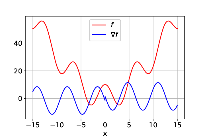
A finite and bounded perturbation should not change the above convergence rate. Indeed, consider the function ϕ⁡(x)=cos⁡(∥x∥){\phi(x)=\cos{(\lVert x\rVert)}}, which is bounded with bounded first derivative. Its gradient is given by ∇ϕ​(x)=−x∥x∥​sin⁡(∥x∥)\nabla\phi(x)=-\frac{x}{\lVert x\rVert}\sin{(\lVert x\rVert)} which is Lipschitz continuous; hence, Lemma 33 implies that it is also β\beta-Hölder continuous. By Lemma 6, the rate obtained from Corollary 4 is applicable to g⁡(x)=∥x∥α+10​cos⁡(∥x∥)+ξ{g(x)=\lVert x\rVert^{\alpha}+10\cos{(\lVert x\rVert)}+\xi}, and the convergence rate 𝒪~​(​d3−αα−1​ϵ−1α−1​){\widetilde{\mathcal{O}}\raisebox{2.15277pt}{\big(}d^{\frac{3-\alpha}{\alpha-1}}\epsilon^{-\frac{1}{\alpha-1}}\raisebox{2.15277pt}{\big)}} still holds. Figure 1(a) demonstrates the behavior of this potential and its gradient when α=1.5{\alpha=1.5}, in 1 dimension.

Refer to caption
(a)
Refer to caption
(b)
Figure 1: (a) Potential f(x)=|x|1.5+10cos(x){f(x)=\mathopen{}\mathclose{{\left|x}}\right|^{1.5}+10\cos{(x)}} and its gradient. The normalizing constant is ignored. (b) Comparison of Growth needed for LSI and this work’s setting, both settings can work with perturbations which are ignored here for clarity.

Example 2 (Smooth potential with linear tails): Since ∥x∥\lVert x\rVert has discontinuous gradient at the origin, we consider f⁡(x)=1+∥x∥2{f(x)=\sqrt{1+\lVert x\rVert^{2}}} as an example of a smooth potential with linear growth. The Hessian of this potential can be computed as

∇2f(x)=(1+∥x∥2CLOSE)−3/2[(1+∥x∥2CLOSE)Id−xx⊤].\nabla^{2}f(x)={{\mathopen{}\mathclose{{\left(1+\lVert x\rVert^{2}}}\right)}^{-3/2}\mathopen{}\mathclose{{\left[\mathopen{}\mathclose{{\left(1+\lVert x\rVert^{2}}}\right){I}_{d}-xx^{\top}}}\right]}.

If we let f~=f{\tilde{f}=f} in Assumption 1, one can easily verify that the assumption holds for θ=3{\theta=3}. Further, computing its gradient reveals that Assumption 2 is satisfied with ζ=0{\zeta=0} and α=1{\alpha=1}. Finally, since its Hessian is bounded, Assumption 3 is satisfied with β=1{\beta=1}. Plugging these parameters in Corollary 4, we obtain the convergence rate OPEN𝒪~​(d7​ϵ−1CLOSE){\widetilde{\mathcal{O}}\mathopen{}\mathclose{{\left(d^{7}\epsilon^{-1}}}\right)} in KL-divergence.

The dimension dependency in the previous convergence rate can be improved by changing f~\tilde{f} to a function that is different than ff. Observe that the difference between 1+∥x∥2\sqrt{1+\lVert x\rVert^{2}} and OPEN(1+∥x∥1+τCLOSE)1/(1+τ){\mathopen{}\mathclose{{\left(1+\lVert x\rVert^{1+\tau}}}\right)^{1/(1+\tau)}} is bounded for any τ∈(0,1){\tau\in(0,1)}. Thus, if we set OPENf~​(x)=(1+∥x∥1+τCLOSE)1/(1+τ){\tilde{f}(x)={\mathopen{}\mathclose{{\left(1+\lVert x\rVert^{1+\tau}}}\right)^{1/(1+\tau)}}}, Assumption 1 is satisfied with θ=2+τ{\theta=2+\tau} and μ=𝒪⁡(τ){\mu=\mathcal{O}(\tau)}. Setting OPENτ=𝒪​(log⁡(6​dCLOSE)−1){\tau=\mathcal{O}({\log\mathopen{}\mathclose{{\left(6d}}\right)}^{-1}}) and invoking Corollary 4 implies a convergence rate of 𝒪~​(d5​ϵ−1){\widetilde{\mathcal{O}}(d^{5}\epsilon^{-1})} in KL-divergence, for a potential like f⁡(x)=1+∥x∥2+0.5​cos⁡(∥x∥){f(x)=\sqrt{1+\lVert x\rVert^{2}}+0.5\cos(\lVert x\rVert)}. We note that in this case, the norm of the perturbation needs to be strictly smaller than 11, otherwise Assumption 2 is no longer satisfied.

Example 3 (Smooth potential with linear tails up to log factor): We consider the potential function OPENf⁡(x)=∥x∥​log⁡(1+∥x∥2CLOSE){f(x)=\lVert x\rVert\log{\mathopen{}\mathclose{{\left(1+\lVert x\rVert^{2}}}\right)}} which is smooth and has a superlinear tail growth. By choosing OPENf~​(x)=log⁡(1+∥x∥2CLOSE)​1+∥x∥2{\tilde{f}(x)=\log{\mathopen{}\mathclose{{\left(1+\lVert x\rVert^{2}}}\right)}\sqrt{1+\lVert x\rVert^{2}}}, one can verify Assumption 1 for θ=1{\theta=1}. Simply calculating the gradient of ff, one can also verify α\alpha-dissipativity (3.3) for α=1\alpha=1. Moreover, ∇f{\nabla f} has logarithmic growth, which means that for any ζ>0{\zeta>0}, gradient growth condition (3.4) holds; thus, Assumption 2 is satisfied. Since ∇f\nabla f is Lipschitz, Assumption 3 is satisfied with β=1\beta=1. Finally, invoking Corollary 4, one obtains a convergence rate of OPEN𝒪~​(d3​ϵ−1CLOSE){\widetilde{\mathcal{O}}\mathopen{}\mathclose{{\left(d^{3}\epsilon^{-1}}}\right)} in KL-divergence.

Comparing the above rate to that in the previous example, we observe that the extra log factor improves the dimension dependence from OPEN𝒪~​(d5CLOSE){\widetilde{\mathcal{O}}\mathopen{}\mathclose{{\left(d^{5}}}\right)} to OPEN𝒪~​(d3CLOSE){\widetilde{\mathcal{O}}\mathopen{}\mathclose{{\left(d^{3}}}\right)}, while the ϵ\epsilon-dependence remains the same. Note that in here α=1\alpha=1, same as in the previous example; yet, the convergence in this case is faster than the advertised rate of 𝒪~​(​dOPEN1β+(1+1β)​(2α−𝟙{α≠1})​ϵ−1β​){\widetilde{\mathcal{O}}\raisebox{2.15277pt}{\big(}d^{\frac{1}{\beta}+(1+\frac{1}{\beta})\mathopen{}\mathclose{{\left(\frac{2}{\alpha}-{\mathbbm{1}}_{\{\alpha\neq 1\}}}}\right)}\epsilon^{-\frac{1}{\beta}}\raisebox{2.15277pt}{\big)}} because the potential is not growing like ∥x∥α\lVert x\rVert^{\alpha} for any α\alpha due to the additional log\log factor. We note that including an extra log factor will only improve the convergence when α=1\alpha=1; when α>1\alpha>1, the convergence rate simply stays the same. One intuitive reason for this phenomenon is that for α>1\alpha>1 the tails are already convex but when α=1\alpha=1, the tails are linear, in which case the Hessian is almost equal to zero, and the extra log\log injects the much needed convexity to the tails.

Figure 1(b) compares the growth rate of these examples with that of the quadratic function, in which case the standard LSI (1.3) holds. Perturbations are ignored to make the figure clear.

5.2 Bayesian regression

In this section, the fixed problem parameters such as MM and LL depend on the data, and the rates are obtained assuming these constants are 𝒪⁡(1)\mathcal{O}(1). Depending on the data scaling, these parameters may depend on the dimension as well as the number of samples nn, in which case the rates can be still obtained by using the explicit formulas presented in Theorem 3 and Corollary 4.

Example 4 (Bridge regression): Our analysis shows that the LMC algorithm can handle potentials that are weakly smooth, which comes up frequently in Bayesian statistics. For example, denoting the matrix of covariates with V={vi}i=1n∈ℝn×d{V=\{v_{i}\}_{i=1}^{n}\in\mathbb{R}^{n\times d}}, and the response vector with Y={yi}i=1n∈ℝn{Y=\{y_{i}\}_{i=1}^{n}\in\mathbb{R}^{n}}, in Bridge linear regression [Fu98, FF93], one assumes the following linear model

Y=V​x+ε where ε∼𝒩⁡(0,In),{Y=Vx+\varepsilon}\quad\text{ where }\quad\varepsilon\sim\mathcal{N}(0,I_{n}),

and a prior proportional to exp(∑i=1d|xi|q){\exp(\sum_{i=1}^{d}\mathopen{}\mathclose{{\left|x_{i}}}\right|^{q})}. Therefore, sampling from the resulting posterior is equivalent to sampling from the following potential function

f(x)=∥Y−Vx∥2+∑i=1d|xi|q.\displaystyle f(x)=\lVert Y-Vx\rVert^{2}+\sum_{i=1}^{d}\mathopen{}\mathclose{{\left|x_{i}}}\right|^{q}.

Assume that we have V⊤​V≻0{V^{\top}V\succ 0} and q∈(1,2)q\in(1,2). Then, the above potential has quadratic growth which, in our framework, translates to setting θ=0{\theta=0} in Assumption 1, and setting α=2{\alpha=2} and ζ=1{\zeta=1} in Assumption 2. This potential lacks smoothness and in the close neighborhood of the origin, Assumption 3 holds with β=q−1\beta=q-1. On the other hand, ∇f\nabla f has linear growth and when ‖x−y‖≥1\|x-y\|\geq 1 Assumption 3 holds with β=1\beta=1. In other words, Assumptions 3 does not hold for a single β\beta for all xx. Initially, it might seem that our results are non-applicable to this potential but by adapting Assumption 3 to this setting as

OPEN∥∇f​(x)−∇f​(y)∥≤L⁡(∥x−y∥β1+∥x−y∥β2CLOSE) for all x,y∈ℝd,\lVert\nabla f(x)-\nabla f(y)\rVert\leq L\mathopen{}\mathclose{{\left(\lVert x-y\rVert^{\beta_{1}}+\lVert x-y\rVert^{\beta_{2}}}}\right)\ \ \text{ for all }\ \ x,y\in\mathbb{R}^{d},

where β1<β2\beta_{1}<\beta_{2}, and some minor changes to Lemma 17, our results can be applied to this potential. In this example, we need to set β1=q−1\beta_{1}=q-1, β2=1\beta_{2}=1, and ζ≤β2\zeta\leq\beta_{2} which yields the convergence rate 𝒪~​(​d1q−1​ϵ−1q−1​){\widetilde{\mathcal{O}}\raisebox{2.15277pt}{\big(}d^{\frac{1}{q-1}}\epsilon^{-\frac{1}{q-1}}\raisebox{2.15277pt}{\big)}} in KL-divergence.

This form of Assumption 3 enables us to deal with composite potentials that are sum of two components each of which is Hölder continuous but with a different exponent.

Example 5 (Bayesian logistic regression): In Bayesian logistic regression, we are given nn samples V={vi}i=1n∈ℝn×d{V=\{v_{i}\}_{i=1}^{n}\in\mathbb{R}^{n\times d}}, Y={yi}i=1n∈{0,1}n{Y=\{y_{i}\}_{i=1}^{n}\in\{0,1\}^{n}} according to the logistic regression model ℙ⁡(yi=1|vi)=1/(1+exp⁡(−⟨x,vi⟩)){\mathbb{P}(y_{i}=1|v_{i})=1/(1+\exp(-{\langle x,v_{i}\rangle}))} for some parameter x∈ℝdx\in\mathbb{R}^{d}, and we would like to make inference about the parameter xx under some prior distribution p⁡(x)p(x). In this framework, it is common to use LMC to generate samples from the posterior distribution p⁡(x|V,Y){p(x|V,Y)} with the following potential function

f⁡(x)=−log⁡p⁡(x)−⟨Y,V​x⟩+∑i=1nlog⁡(1+exp⁡(⟨x,vi⟩)).\displaystyle f(x)=-\log{p(x)}-{\langle Y,Vx\rangle}+\sum_{i=1}^{n}\log(1+\exp({\langle x,v_{i}\rangle})). (5.1)

In practice, the prior distribution can be arbitrary whereas most theoretical results require the prior to be the Gaussian distribution in order to ensure that the posterior is smooth and has quadratic growth [Dal17b, LWME19]. The framework in this paper allows for priors that have heavier tails than a Gaussian and/or have potentials that do not have Lipschitz gradients. For example, consider a pseudo-Huber prior p⁡(x)∝exp⁡(1−1+∥x∥2){p(x)\propto\exp\big(1-\sqrt{1+\lVert x\rVert^{2}}\big)} [GDV+19, HZ03], which results in a similar setting as in Example 2 in the sense that simply choosing f~\tilde{f} as the potential yields an OPEN𝒪~​(d7​ϵ−1CLOSE){\widetilde{\mathcal{O}}\mathopen{}\mathclose{{\left(d^{7}\epsilon^{-1}}}\right)} convergence rate in KL-divergence. As before, the dimension dependency can be improved by a more careful choice of f~\tilde{f}, i.e.,

OPENf~​(x)=(1+∥x∥1+τCLOSE)1/(1+τ)−⟨Y,V​x⟩+∑i=1nlog⁡(1+exp⁡(⟨x,vi⟩)),\displaystyle\tilde{f}(x)={\mathopen{}\mathclose{{\left(1+\lVert x\rVert^{1+\tau}}}\right)^{1/(1+\tau)}}-{\langle Y,Vx\rangle}+\sum_{i=1}^{n}\log(1+\exp({\langle x,v_{i}\rangle})),

which yields a convergence rate of OPEN𝒪~​(d5​ϵ−1CLOSE){\widetilde{\mathcal{O}}\mathopen{}\mathclose{{\left(d^{5}\epsilon^{-1}}}\right)}. In here the parameters are set as follows θ=2+τ\theta=2+\tau, α=1\alpha=1, ζ=0\zeta=0 and β=1\beta=1.

Next, consider the prior p(x)∝exp(∑i=1d|xi|q){p(x)\propto\exp\big(\sum_{i=1}^{d}\mathopen{}\mathclose{{\left|x_{i}}}\right|^{q}\big)} for q∈(1,2)q\in(1,2) which is similar to the Bridge linear regression setting. The resulting potential is not smooth in this case, and the potential lacks quadratic growth. Our analysis shows that LMC reaches ϵ\epsilon-accuracy in KL-divergence after 𝒪~​(​d3−qq−1​ϵ−1q−1​){\widetilde{\mathcal{O}}\raisebox{2.15277pt}{\big(}d^{\frac{3-q}{q-1}}\epsilon^{-\frac{1}{q-1}}\raisebox{2.15277pt}{\big)}} steps. Here, the parameters are given as θ=2−q\theta=2-q, α=q\alpha=q, ζ=q−1\zeta=q-1, and β=q−1\beta=q-1.

Example 6 (Huberized Regression with log-linear prior): Let VV and YY denote the matrix of covariates and the response vector respectively, as in Example 4. We consider the Bayesian analog of Huberized loss [PC08] with a log-linear prior, which corresponds to sampling from the posterior p⁡(x)∝e−f⁡(x)p(x)\propto e^{-f(x)} where

f⁡(x)=∑i=1nOPEN1+(yi−⟨x,vi⟩CLOSE)2+1+∥x∥2.\displaystyle f(x)=\sum_{i=1}^{n}\sqrt{1+\mathopen{}\mathclose{{\left(y_{i}-{\langle x,v_{i}\rangle}}}\right)^{2}}+\sqrt{1+\lVert x\rVert^{2}}.

By considering

OPENf~​(x)=∑i=1nOPEN1+(yi−⟨x,vi⟩CLOSE)2+(1+∥x∥1+τCLOSE)11+τ,\displaystyle\tilde{f}(x)=\sum_{i=1}^{n}\sqrt{1+\mathopen{}\mathclose{{\left(y_{i}-{\langle x,v_{i}\rangle}}}\right)^{2}}+\mathopen{}\mathclose{{\left(1+\lVert x\rVert^{1+\tau}}}\right)^{\frac{1}{1+\tau}},

for τ∈(0,1)\tau\in(0,1) and applying an argument similar to the one in Example 2, one can obtain the convergence rate OPEN𝒪~​(d5​ϵ−1CLOSE){\widetilde{\mathcal{O}}\mathopen{}\mathclose{{\left(d^{5}\epsilon^{-1}}}\right)} for the LMC algorithm in KL-divergence. In here, the parameters are given as θ=2+τ\theta=2+\tau, α=1\alpha=1, ζ=0\zeta=0 and β=1\beta=1.

6 Proof of Modified Log-Sobolev Inequality

We start with a lemma that allows us to construct a finite perturbation of the potential function that has polynomially decaying Hessian which is unbounded at 0. This will allow us to optimize the final bound.

Lemma 10.

Suppose Assumption 1 holds. Then for sufficiently small ε>0{\varepsilon>0}, there exist a function f~ε:ℝd→ℝ{\tilde{f}_{\varepsilon}:\mathbb{R}^{d}\to\mathbb{R}} such that

‖f−f~ε‖∞≤ξ+ε/2,\big\|f-\tilde{f}_{\varepsilon}\big\|_{\infty}\leq\xi+\varepsilon/2,

where f~ε\tilde{f}_{\varepsilon} satisfies,

∇2f~ε​(x)⪰m⁡(‖x‖)​Id,\displaystyle\nabla^{2}\tilde{f}_{\varepsilon}(x)\succeq m(\|x\|){I}_{d}, (6.1)

where m:ℝ+→ℝ+{m:\mathbb{R}_{+}\to\mathbb{R}_{+}} is a monotonically decreasing and onto function satisfying

m⁡(r)≥μ−αθ​ε(1+r2/4)θ/2,{m(r)\geq\frac{\mu-\alpha_{\theta}\varepsilon}{(1+r^{2}/4)^{\theta/2}}},

where αθ<∞{\alpha_{\theta}<\infty} is a constant depending only on θ\theta.

Proof of Lemma 10. Let f~ε​(x)=f~​(x)+ε​∥x∥3/2​e−∥x∥2\tilde{f}_{\varepsilon}(x)=\tilde{f}(x)+\varepsilon\lVert x\rVert^{3/2}e^{-\lVert x\rVert^{2}}, and notice that ff satisfies

∥f−f~ε∥∞≤ξ+ε/2.{\lVert f-\tilde{f}_{\varepsilon}\rVert_{\infty}\leq\xi+\varepsilon/2}.

For its Hessian, we write

∇2f~ε(x)=∇2f~(x)+εe−∥x∥2{(32∥x∥−1/2−2∥x∥3/2)Id−(6∥x∥−1/2−4∥x∥3/2+34∥x∥−5/2)xx⊤}\displaystyle\nabla^{2}\tilde{f}_{\varepsilon}(x)=\nabla^{2}\tilde{f}(x)+\varepsilon e^{-\lVert x\rVert^{2}}\mathopen{}\mathclose{{\left\{\mathopen{}\mathclose{{\left(\frac{3}{2}\lVert x\rVert^{-1/2}-2\lVert x\rVert^{3/2}}}\right){I}_{d}-\mathopen{}\mathclose{{\left(6\lVert x\rVert^{-1/2}-4\lVert x\rVert^{3/2}+\frac{3}{4}\lVert x\rVert^{-5/2}}}\right)xx^{\top}}}\right\}

and choosing αθ=8​supr≥0r1.5​(1+r2/4)θ/2​e−r2{\alpha_{\theta}=8\sup_{r\geq 0}r^{1.5}(1+r^{2}/4)^{\theta/2}e^{-r^{2}}}, we observe that

∇2f~ε​(x)⪰μ−αθ​ε(1+∥x∥2/4)θ/2​Id.{\nabla^{2}\tilde{f}_{\varepsilon}(x)\succeq\frac{\mu-\alpha_{\theta}\varepsilon}{(1+\lVert x\rVert^{2}/4)^{\theta/2}}}{I}_{d}.

Also, ∇2f~ε(x)>ε∥x∥−1/2/2{\nabla^{2}\tilde{f}_{\varepsilon}(x)>\varepsilon\lVert x\rVert^{-1/2}/2} when x≤0.1{x\leq 0.1}. Now by selecting

m(r)=(μ−αθε)(1+r2/4)−θ/2∨ε2r−1/2𝟙{r≤0.1},{m(r)=(\mu-\alpha_{\theta}\varepsilon)(1+r^{2}/4)^{-\theta/2}\vee\frac{\varepsilon}{2}r^{-1/2}{\mathbbm{1}}_{\{r\leq 0.1\}}},

the lemma follows. Note that m:ℝ+→ℝ{m:\mathbb{R}_{+}\to\mathbb{R}} is both monotone and onto for ε<1/(αθ+2){\varepsilon<{1}/{(\alpha_{\theta}+2)}}. ∎

Proof of Theorem 1. We follow a similar construction developed in [TV00], and define the functions hh and h~ε\tilde{h}_{\varepsilon} as

h(x)=f(x)+m(2r)(∥x∥−r)2𝟙{∥x∥≥r}+Cr and\displaystyle h(x)=f(x)+m(2r)\big(\lVert x\rVert-r\big)^{2}{\mathbbm{1}}_{\{\lVert x\rVert\geq r\}}+C_{r}\ \text{ and } (6.2)
h~ε(x)=f~ε(x)+m(2r)(∥x∥−r)2𝟙{∥x∥≥r}+Cr,\displaystyle\tilde{h}_{\varepsilon}(x)=\tilde{f}_{\varepsilon}(x)+m(2r)\big(\lVert x\rVert-r\big)^{2}{\mathbbm{1}}_{\{\lVert x\rVert\geq r\}}+C_{r}, (6.3)

where CrC_{r} is the normalizing constant for the unnormalized potential hh satisfying

eCr=∫∥x∥<re−f⁡(x)​𝑑x+∫∥x∥≥re−f⁡(x)​e−m⁡(2​r)​(∥x∥−r)2​𝑑x.e^{C_{r}}=\int_{\lVert x\rVert<r}e^{-f(x)}dx+\int_{\lVert x\rVert\geq r}e^{-f(x)}e^{-m(2r)(\lVert x\rVert-r)^{2}}dx. (6.4)

Using Assumption 1 and Lemma 10, we notice that hh and h~ε\tilde{h}_{\varepsilon} satisfy |h⁡(x)−h~ε​(x)|≤ξ+ε/2{\big|h(x)-\tilde{h}_{\varepsilon}(x)\big|\leq\xi+\varepsilon/2}, and also the growth of the function h~ε\tilde{h}_{\varepsilon} can be characterized in the following three regions.

  • •

    For ∥x∥<r{\lVert x\rVert<r}, we have

    ∇2h~ε​(x)=∇2f~ε​(x)⪰\displaystyle\nabla^{2}\tilde{h}_{\varepsilon}(x)=\nabla^{2}\tilde{f}_{\varepsilon}(x)\succeq m⁡(∥x∥)​Id\displaystyle m(\lVert x\rVert){I}_{d}
    ⪰\displaystyle\succeq m⁡(2​r)​Id,\displaystyle m(2r){I}_{d},

    where in the last step we used the monotonicity of mm.

  • •

    For r≤∥x∥<2​r{r\leq\lVert x\rVert<2r}, we have

    ∇2h~ε​(x)=∇2f~ε(x)+m(2r){2Id−2​r∥x∥Id+2rx​x⊤∥x∥3}⪰m(∥x∥)Id+m(2r){2Id−2Id+0}⪰m⁡(2​r)​Id,\begin{split}\nabla^{2}\tilde{h}_{\varepsilon}(x)=&\nabla^{2}\tilde{f}_{\varepsilon}(x)+m(2r)\mathopen{}\mathclose{{\left\{2{I}_{d}-\frac{2r}{\lVert x\rVert}{I}_{d}+2r\frac{xx^{\top}}{\lVert x\rVert^{3}}}}\right\}\\ \succeq&m(\lVert x\rVert){I}_{d}+{m(2r)}\mathopen{}\mathclose{{\left\{2{I}_{d}-2{I}_{d}+0}}\right\}\\ \succeq&m(2r){I}_{d},\end{split}

    where again the last step follows from the monotonicity of mm.

  • •

    For 2​r≤∥x∥{2r\leq\lVert x\rVert}, we have

    ∇2h~ε​(x)=∇2f~ε(x)+m(2r){2Id−2​r∥x∥Id+2rx​x⊤∥x∥3}⪰0+m(2r){2Id−Id+0}⪰m⁡(2​r)​Id.\begin{split}\nabla^{2}\tilde{h}_{\varepsilon}(x)=&\nabla^{2}\tilde{f}_{\varepsilon}(x)+{m(2r)}\mathopen{}\mathclose{{\left\{2{I}_{d}-\frac{2r}{\lVert x\rVert}{I}_{d}+2r\frac{xx^{\top}}{\lVert x\rVert^{3}}}}\right\}\\ \succeq&0+{m(2r)}\mathopen{}\mathclose{{\left\{2{I}_{d}-{I}_{d}+0}}\right\}\\ \succeq&{m(2r)}{I}_{d}.\end{split}

In all three cases, we obtain that the function h~ε\tilde{h}_{\varepsilon} has a positive definite Hessian which is lower bounded by m⁡(2​r){m(2r)} which implies, by the Bakry-Emery’s LSI result on strongly convex potentials [BE85] that the distribution e−h~εe^{-\tilde{h}_{\varepsilon}} satisfies (1.3). Combining this with the Holley-Stroock perturbation lemma [HS87], we obtain

∀ρ,H​(ρ|e−h)≤e2​ξ+ε2​m​(2​r)​I​(ρ|e−h).\forall\rho,\ \ \textnormal{H}\big({\rho}|{e^{-h}}\big)\leq\frac{e^{2\xi+\varepsilon}}{2m(2r)}\textnormal{I}\big({\rho}|{e^{-h}}\big). (6.5)

We will convert the above inequality on the perturbed potential hh to an inequality on the potential function ff. Using the definition in (6.2), we can obtain an upper bound on the relative entropy for all r>0{r>0},

H​(ρ|e−f)=\displaystyle\textnormal{H}\big({\rho}|{e^{-f}}\big)= H​(ρ|e−h)+∫ρ⁡(x)​(f⁡(x)−h⁡(x))​𝑑x\displaystyle\textnormal{H}\big({\rho}|{e^{-h}}\big)+\int\rho(x)(f(x)-h(x))dx (6.6)
=\displaystyle= H​(ρ|e−h)−m⁡(2​r)​∫∥x∥≥rρ⁡(x)​(‖x‖−r)2​𝑑x−Cr.\displaystyle\textnormal{H}\big({\rho}|{e^{-h}}\big)-{m(2r)}\int_{\lVert x\rVert\geq r}\rho(x)(\|x\|-r)^{2}dx-C_{r}. (6.7)

For the normalizing constant CrC_{r} explicitly given in (6.4), one can obtain a lower bound using the Jensen’s inequality,

Cr=\displaystyle C_{r}= log∫e−f⁡(x)e−m(2r)(∥x∥−r)2𝟙{∥x∥≥r}dx\displaystyle\log\int e^{-f(x)}e^{-{m(2r)}(\lVert x\rVert-r)^{2}{\mathbbm{1}}_{\{\|x\|\geq r\}}}dx (6.8)
≥\displaystyle\geq −m(2r)∫‖x‖≥re−f⁡(x)(∥x∥−r)2dx.\displaystyle-{m(2r)}\int_{\|x\|\geq r}e^{-f(x)}(\lVert x\rVert-r)^{2}dx. (6.9)

Combining this with (6.6), we obtain

H​(ρ|e−f)≤\displaystyle\textnormal{H}\big({\rho}|{e^{-f}}\big)\leq H​(ρ|e−h)+m⁡(2​r)​∫∥x∥≥r(e−f⁡(x)−ρ⁡(x))​(‖x‖−r)2​𝑑x\displaystyle\textnormal{H}\big({\rho}|{e^{-h}}\big)+{m(2r)}\int_{\lVert x\rVert\geq r}\big(e^{-f(x)}-\rho(x)\big)(\|x\|-r)^{2}dx (6.10)
≤\displaystyle\leq H​(ρ|e−h)+m⁡(2​r)​∫∥x∥≥re−f⁡(x)​‖x‖2​𝑑x\displaystyle\textnormal{H}\big({\rho}|{e^{-h}}\big)+{m(2r)}\int_{\lVert x\rVert\geq r}e^{-f(x)}\|x\|^{2}dx (6.11)
≤\displaystyle\leq H​(ρ|e−h)+m⁡(2​r)​Ms​(ν∗)(1+r2)s/2−1\displaystyle\textnormal{H}\big({\rho}|{e^{-h}}\big)+{m(2r)}\frac{\textnormal{M}_{s}(\nu_{*})}{(1+r^{2})^{s/2-1}} (6.12)

where the second step follows since ρ≥0{\rho\geq 0}, and ‖x‖2≥(‖x‖−r)2{\|x\|^{2}\geq(\|x\|-r)^{2}} in the domain of integration, and the last step follows from Lemma 11 below.

Lemma 11.

For a given distribution ρ\rho and for a constant r>0{r>0}, we have

∫‖x‖≥rρ⁡(x)​‖x‖2​𝑑x≤Ms​(ρ)(1+r2)s/2−1.\displaystyle\int_{\|x\|\geq r}\rho(x)\|x\|^{2}dx\leq\frac{\textnormal{M}_{s}(\rho)}{(1+r^{2})^{s/2-1}}. (6.13)

Proof of Lemma 11. For positive constants p,q,s>0{p,q,s>0} satisfying 1/p+1/q=1{1/p+1/q=1}, we apply the Hölder’s inequality and get

∫‖x‖≥rρ⁡(x)​‖x‖2​𝑑x=\displaystyle\int_{\|x\|\geq r}\rho(x)\|x\|^{2}dx= ∫ρ(x)∥x∥2𝟙{∥x∥≥r}dx\displaystyle\int\rho(x)\|x\|^{2}{\mathbbm{1}}_{\{\|x\|\geq r\}}dx (6.14)
≤\displaystyle\leq (∫ρ⁡(x)​‖x‖2​p​𝑑xCLOSE)1/pℙ((1+‖x‖2CLOSE)s/2≥(1+r2)s/2)1/q\displaystyle\mathopen{}\mathclose{{\left(\int\rho(x)\|x\|^{2p}dx}}\right)^{{1}/{p}}\mathbb{P}\mathopen{}\mathclose{{\left(\mathopen{}\mathclose{{\left(1+\|x\|^{2}}}\right)^{s/2}\geq{(1+r^{2})^{s/2}}}}\right)^{1/q} (6.15)
≤\displaystyle\leq M2​p​(ρ)1/p​Ms​(ρ)1/q(1+r2)s/2​q,\displaystyle\frac{\textnormal{M}_{2p}(\rho)^{{1}/{p}}\textnormal{M}_{s}(\rho)^{1/q}}{(1+r^{2})^{s/2q}}, (6.16)

where the last step follows from Markov’s inequality. Final result follows by choosing p=s/2{p=s/2}. ∎

Similarly for the Fisher information, we write

I​(ρ|e−h)≤2​I​(ρ|e−f)+2​∫ρ⁡(x)​∥∇h​(x)−∇f​(x)∥2​𝑑x.\displaystyle\textnormal{I}\big({\rho}|{e^{-h}}\big)\leq 2\textnormal{I}\big({\rho}|{e^{-f}}\big)+2\int\rho(x)\lVert\nabla h(x)-\nabla f(x)\rVert^{2}dx. (6.17)

For the second term on the right hand side, we write

∫ρ⁡(x)​∥∇h​(x)−∇f​(x)∥2​𝑑x=\displaystyle\int\rho(x)\lVert\nabla h(x)-\nabla f(x)\rVert^{2}dx= 4m(2r)2∫ρ(x)(∥x∥−r)2𝟙{∥x∥≥r}dx\displaystyle 4m(2r)^{2}\int\rho(x)(\lVert x\rVert-r)^{2}{\mathbbm{1}}_{\{\lVert x\rVert\geq r\}}dx (6.18)
≤\displaystyle\leq 4m(2r)2∫ρ(x)∥x∥2𝟙{∥x∥≥r}dx\displaystyle 4m(2r)^{2}\int\rho(x)\lVert x\rVert^{2}{\mathbbm{1}}_{\{\lVert x\rVert\geq r\}}dx (6.19)
≤\displaystyle\leq 4​m​(2​r)2(1+r2)s/2−1​Ms​(ρ),\displaystyle\frac{4m(2r)^{2}}{(1+r^{2})^{s/2-1}}\textnormal{M}_{s}(\rho), (6.20)

where in the last step we applied Lemma 11. Plugging this back in (6.17), we get

I​(ρ|e−h)≤2​I​(ρ|e−f)+8​m​(2​r)2(1+r2)s/2−1​Ms​(ρ).\displaystyle\textnormal{I}\big({\rho}|{e^{-h}}\big)\leq 2\textnormal{I}\big({\rho}|{e^{-f}}\big)+\frac{8m(2r)^{2}}{(1+r^{2})^{s/2-1}}\textnormal{M}_{s}(\rho). (6.21)

Combining the inequalities (6.5), (6.12), and (6.21), we obtain

∀ρ,H​(ρ|e−f)≤\displaystyle\forall\rho,\ \ \textnormal{H}\big({\rho}|{e^{-f}}\big)\leq H​(ρ|e−h)+m⁡(2​r)​Ms​(ν∗)(1+r2)s/2−1\displaystyle\textnormal{H}\big({\rho}|{e^{-h}}\big)+\frac{m(2r)\textnormal{M}_{s}(\nu_{*})}{(1+r^{2})^{s/2-1}} (6.22)
≤\displaystyle\leq e2​ξ+ε2​m​(2​r)​I​(ρ|e−h)+m⁡(2​r)​Ms​(ν∗)(1+r2)s/2−1\displaystyle\frac{e^{2\xi+\varepsilon}}{2m(2r)}\textnormal{I}\big({\rho}|{e^{-h}}\big)+\frac{m(2r)\textnormal{M}_{s}(\nu_{*})}{(1+r^{2})^{s/2-1}} (6.23)
≤\displaystyle\leq OPENe2​ξ+εm⁡(2​r)​I​(ρ|e−f)+m⁡(2​r)(1+r2)s/2−1​(4​e2​ξ+ε​Ms​(ρ)+Ms​(ν∗)CLOSE)\displaystyle\frac{e^{2\xi+\varepsilon}}{m(2r)}\textnormal{I}\big({\rho}|{e^{-f}}\big)+\frac{m(2r)}{(1+r^{2})^{s/2-1}}\mathopen{}\mathclose{{\left(4e^{2\xi+\varepsilon}\textnormal{M}_{s}(\rho)+\textnormal{M}_{s}(\nu_{*})}}\right) (6.24)
≤\displaystyle\leq e2​ξ+εm⁡(2​r)​I​(ρ|e−f)+4​e2​ξ+ε​m⁡(2​r)(1+r2)s/2−1​Ms​(ρ+ν∗).\displaystyle\frac{e^{2\xi+\varepsilon}}{m(2r)}\textnormal{I}\big({\rho}|{e^{-f}}\big)+4e^{2\xi+\varepsilon}\frac{m(2r)}{(1+r^{2})^{s/2-1}}\textnormal{M}_{s}(\rho+\nu_{*}). (6.25)

Finally, using the Lemma 27 and optimizing over m⁡(2​r){m(2r)}, we get

∀ρ,H​(ρ|e−f)≤\displaystyle\forall\rho,\ \ \textnormal{H}\big({\rho}|{e^{-f}}\big)\leq λε​I​(ρ|e−f)s−2+θs−2+2​θ​Ms​(ρ+ν∗)θs−2+2​θ,\displaystyle\lambda_{\varepsilon}\textnormal{I}\big({\rho}|{e^{-f}}\big)^{\frac{s-2+\theta}{s-2+2\theta}}\textnormal{M}_{s}(\rho+\nu_{*})^{\frac{\theta}{s-2+2\theta}}, (6.26)

where

λε=4​e2​ξ+ε(μ−αθ​ε)s−2s−2+2​θ,\displaystyle\lambda_{\varepsilon}=\frac{4e^{2\xi+\varepsilon}}{(\mu-\alpha_{\theta}\varepsilon)^{\frac{s-2}{s-2+2\theta}}}, (6.27)

for all sufficiently small ε>0{\varepsilon>0}. Taking the limit of ε↓0{\varepsilon\downarrow 0} concludes the proof. ∎

7 Moment Bounds on the LMC Iterates

Proof of Proposition 2. Similar to the continuous-time case, it suffices to prove

Ms​(ρk)≤Ms​(ρ0)+Cs​k​η.\displaystyle\textnormal{M}_{s}(\rho_{k})\leq\textnormal{M}_{s}(\rho_{0})+C_{s}k\eta.

Part 1. We prove a linear bound on the second moment of x~k,t\widetilde{x}_{k,t} conditioned on xkx_{k}. Consider the distribution ρ(x~k,t|xk){\rho(\widetilde{x}_{k,t}\rvert x_{k})} which is the distribution of x~k,t\widetilde{x}_{k,t} given xkx_{k}.

𝔼[∥x~k,t∥2|xk]=∥xk∥2−2t⟨∇f(xk),xk⟩+t2∥∇f(xk)∥2+2dt≤1∥xk∥2−2​t​(a​∥xk∥α−b)+2​t2​M2​(1+∥xk∥2​ζ)+2​d​t=∥xk∥2+2t(−a⁡(1+∥xk∥αCLOSE)+η​M2​∥xk∥2​ζ+a+b+d+η​M2)OPEN≤2∥xk∥2+2​(a+b+d+η​M2CLOSE)​t≤∥xk∥2+C2​t,\begin{split}\mathbb{E}\mathopen{}\mathclose{{\left[\lVert\widetilde{x}_{k,t}\rVert^{2}\rvert x_{k}}}\right]&=\lVert x_{k}\rVert^{2}-2t\mathopen{}\mathclose{{\left<\nabla f(x_{k}),x_{k}}}\right>+t^{2}\lVert\nabla{f(x_{k})}\rVert^{2}+2dt\\ &\stackrel{{\scriptstyle 1}}{{\leq}}\lVert x_{k}\rVert^{2}-2t(a\lVert x_{k}\rVert^{\alpha}-b)+2t^{2}M^{2}(1+\lVert x_{k}\rVert^{2\zeta})+2dt\\ &=\lVert x_{k}\rVert^{2}+2t\mathopen{}\mathclose{{\left(-a\mathopen{}\mathclose{{\left(1+\lVert x_{k}\rVert^{\alpha}}}\right)+\eta M^{2}\lVert x_{k}\rVert^{2\zeta}+a+b+d+\eta M^{2}}}\right)\\ &\stackrel{{\scriptstyle 2}}{{\leq}}\lVert x_{k}\rVert^{2}+2\mathopen{}\mathclose{{\left(a+b+d+\eta M^{2}}}\right)t\\ &\leq\lVert x_{k}\rVert^{2}+C_{2}t,\end{split}

for any C2C_{2} satisfying

C2≥3​a+2​b+2​d.C_{2}\geq 3a+2b+2d. (7.1)

Step 1 is obtained using Assumptions 2, and step 2 is because 4​η​M2≤a{4\eta M^{2}\leq a}. Adding one to both sides, we get the following equation

M2(ρ~k,t|xk)≤g2(xk)+C2t,\textnormal{M}_{2}(\widetilde{\rho}_{k,t}\rvert x_{k})\leq g_{2}(x_{k})+C_{2}t, (7.2)

where OPENgs​(x)=(1+x2CLOSE)s/2{g_{s}(x)=\mathopen{}\mathclose{{\left(1+x^{2}}}\right)^{s/2}} and Ms(ρ~k,t|xk){\textnormal{M}_{s}(\widetilde{\rho}_{k,t}\rvert x_{k})} denotes the ss-moment of x~k,t\widetilde{x}_{k,t} conditioned on xkx_{k}.

Part 2. We upper bound a term which will become useful in the proof of the induction step. (In below, ZZ denotes a standard Gaussian vector that is independent of xkx_{k}.)

𝔼[−⟨∇f(xk),Z⟩g2(x~k,t)|xk]=122​t𝔼[−⟨∇f(xk),Z⟩⟨xk,Z⟩+t⟨∇f(xk),Z⟩⟨∇f(xk),Z⟩|xk]OPEN=2​2​t​(−⟨∇f(xk),xk⟩+t∥∇f(xk)∥2)OPEN≤2​2​η​(−a​∥xk∥α+b+2​η​M2​(1+∥xk∥2​ζ)CLOSE)≤22​η(−a⁡(∥xk∥α+1CLOSE)+2​η​M2​∥xk∥2​ζ+a+b+2​η​M2)OPEN≤22​2​η​(a+b+2​η​M2CLOSE)≤N2,\begin{split}\mathbb{E}\mathopen{}\mathclose{{\left[-\mathopen{}\mathclose{{\left<\nabla f(x_{k}),Z}}\right>g_{2}(\widetilde{x}_{k,t})\rvert x_{k}}}\right]&\stackrel{{\scriptstyle 1}}{{=}}2\sqrt{2t}\mathbb{E}\mathopen{}\mathclose{{\left[-\mathopen{}\mathclose{{\left<\nabla f(x_{k}),Z}}\right>\mathopen{}\mathclose{{\left<x_{k},Z}}\right>+t\mathopen{}\mathclose{{\left<\nabla f(x_{k}),Z}}\right>\mathopen{}\mathclose{{\left<\nabla f(x_{k}),Z}}\right>\rvert x_{k}}}\right]\\ &=2\sqrt{2t}\mathopen{}\mathclose{{\left(-\mathopen{}\mathclose{{\left<\nabla f(x_{k}),x_{k}}}\right>+t\lVert\nabla{f(x_{k})}\rVert^{2}}}\right)\\ &\leq 2\sqrt{2\eta}\mathopen{}\mathclose{{\left(-a\lVert x_{k}\rVert^{\alpha}+b+2\eta M^{2}(1+\lVert x_{k}\rVert^{2\zeta})}}\right)\\ &\leq 2\sqrt{2\eta}\mathopen{}\mathclose{{\left(-a\mathopen{}\mathclose{{\left(\lVert x_{k}\rVert^{\alpha}+1}}\right)+2\eta M^{2}\lVert x_{k}\rVert^{2\zeta}+a+b+2\eta M^{2}}}\right)\\ &\stackrel{{\scriptstyle 2}}{{\leq}}2\sqrt{2\eta}\mathopen{}\mathclose{{\left(a+b+2\eta M^{2}}}\right)\leq N_{2},\end{split}

where

OPENN2≜2​2​η​(1.5​a+bCLOSE).N_{2}\triangleq 2\sqrt{2\eta}\mathopen{}\mathclose{{\left(1.5a+b}}\right). (7.3)

Step 1 follows from odd Gaussian moments being zero, and step 2 uses 4​η​M2<a{4\eta M^{2}<a}. Note that ZZ is independent of xkx_{k}, with zero mean.

Part 3. Now we use induction to prove the linear bound for even moments of the conditional distribution. The base case (s=2{s=2}) is already proved. Hence we can assume s≥4{s\geq 4} which implies (s−4){(s-4)} is an even non-negative integer. For the proof to work, we need to strengthen the induction hypothesis for which part 2 in the proof will be useful. For all even ss, we have

  1. 1.

    Ms(ρ~k,t|xk)≤gs(xk)+Cst.{\textnormal{M}_{s}(\widetilde{\rho}_{k,t}\rvert x_{k})\leq g_{s}(x_{k})+C_{s}t}.

  2. 2.

    𝔼[−⟨∇f(xk),Z⟩gs(x~k,t)|xk]≤Ns.{\mathbb{E}\mathopen{}\mathclose{{\left[-\mathopen{}\mathclose{{\left<\nabla f(x_{k}),Z}}\right>g_{s}(\widetilde{x}_{k,t})\rvert x_{k}}}\right]\leq N_{s}}.

For the first inequality above, we will bound the time derivative of Ms(ρ~k,t|xk){\textnormal{M}_{s}(\widetilde{\rho}_{k,t}\rvert x_{k})} as follows.

∂∂t​Ms​(CLOSEρ~k,t|xk)=𝔼[−s⟨∇f(xk),x~k,t⟩gs−2(x~k,t)+s(d+s−2)gs−2(x~k,t)−s(s−2)gs−4(x~k,t)|xk]≤s𝔼[(−⟨∇f(xk),xk−t∇f(xk)+2​tZ⟩+(d+s−2))gs−2(x~k,t)|xk]≤s(−⟨∇f(xk),xk⟩+t∥∇f(xk)∥2+(d+s−2))𝔼[gs−2(x~k,t)|xk]+s2​t𝔼[⟨−∇f(xk),Z⟩gs−2(x~k,t)|xk]≤s[−a∥xk∥α+b+2ηM2(1+∥xk∥2​ζ)+(d+s−2)]+(gs−2(xk)+Cs−2t)+s2​ηNs−2≤s[−a(1+∥xk∥2)α2+2ηM2(1+∥xk∥2)ζ+(2ηM2+a+b+d+s−2)]+(gs−2(xk)+Cs−2t)+s​2​η​Ns−2OPEN≤1maxu≥1⁡s⁡(−a​uα+2​η​M2​u2​ζ+(2​η​M2+a+b+d+s−2)CLOSE)​(us−2+Cs−2​t)+s​2​η​Ns−2OPEN≤s​maxu≥1​(−a2​uα+s−2+2​η​M2​u2​ζ+s−2CLOSE)OPEN+s​maxu≥1​(−a2​uα+s−2+(2​η​M2+a+b+d+s−2)​us−2CLOSE)OPEN+s​Cs−2​η​maxu≥1​(−a​uα+2​η​M2​u2​ζ+(2​η​M2+a+b+d+s−2)CLOSE)+s​2​η​Ns−2≤2s[(2ηM2+a+b+d+s−2)(2​(2​η​M2+a+b+d+s−2)​(s−2)a⁡(α+s−2)CLOSE)s−2α+Cs−2η(2ηM2+a+b+d+s−2)+2​ηNs−2],\begin{split}\frac{\partial}{\partial t}\textnormal{M}_{s}(&\widetilde{\rho}_{k,t}\rvert x_{k})\\ &=\mathbb{E}\mathopen{}\mathclose{{\left[-s\mathopen{}\mathclose{{\left<\nabla f(x_{k}),\widetilde{x}_{k,t}}}\right>g_{s-2}(\widetilde{x}_{k,t})+s(d+s-2)g_{s-2}(\widetilde{x}_{k,t})-s(s-2)g_{s-4}(\widetilde{x}_{k,t})\rvert x_{k}}}\right]\\ &\leq s\mathbb{E}\mathopen{}\mathclose{{\left[\mathopen{}\mathclose{{\left(-\mathopen{}\mathclose{{\left<\nabla f(x_{k}),x_{k}-t\nabla f(x_{k})+\sqrt{2t}Z}}\right>+(d+s-2)}}\right)g_{s-2}(\widetilde{x}_{k,t})\rvert x_{k}}}\right]\\ &\leq s\mathopen{}\mathclose{{\left(-\mathopen{}\mathclose{{\left<\nabla f(x_{k}),x_{k}}}\right>+t\lVert\nabla f(x_{k})\rVert^{2}+(d+s-2)}}\right)\mathbb{E}\mathopen{}\mathclose{{\left[g_{s-2}(\widetilde{x}_{k,t})\rvert x_{k}}}\right]\\ &\qquad+s\sqrt{2t}\mathbb{E}\mathopen{}\mathclose{{\left[\mathopen{}\mathclose{{\left<-\nabla f(x_{k}),Z}}\right>g_{s-2}(\widetilde{x}_{k,t})\rvert x_{k}}}\right]\\ &\leq s\mathopen{}\mathclose{{\left[-a\lVert x_{k}\rVert^{\alpha}+b+2\eta M^{2}(1+\lVert x_{k}\rVert^{2\zeta})+(d+s-2)}}\right]_{+}(g_{s-2}(x_{k})+C_{s-2}t)+s\sqrt{2\eta}N_{s-2}\\ &\leq s\mathopen{}\mathclose{{\left[-a(1+\lVert x_{k}\rVert^{2})^{\frac{\alpha}{2}}+2\eta M^{2}(1+\lVert x_{k}\rVert^{2})^{\zeta}+(2\eta M^{2}+a+b+d+s-2)}}\right]_{+}(g_{s-2}(x_{k})+C_{s-2}t)\\ &\qquad+s\sqrt{2\eta}N_{s-2}\\ &\stackrel{{\scriptstyle 1}}{{\leq}}\max_{u\geq 1}s\mathopen{}\mathclose{{\left(-au^{\alpha}+2\eta M^{2}u^{2\zeta}+(2\eta M^{2}+a+b+d+s-2)}}\right)(u^{s-2}+C_{s-2}t)+s\sqrt{2\eta}N_{s-2}\\ &\leq s\max_{u\geq 1}\mathopen{}\mathclose{{\left(-\frac{a}{2}u^{\alpha+s-2}+2\eta M^{2}u^{2\zeta+s-2}}}\right)\\ &\qquad+s\max_{u\geq 1}\mathopen{}\mathclose{{\left(-\frac{a}{2}u^{\alpha+s-2}+(2\eta M^{2}+a+b+d+s-2)u^{s-2}}}\right)\\ &\qquad+sC_{s-2}\eta\max_{u\geq 1}\mathopen{}\mathclose{{\left(-au^{\alpha}+2\eta M^{2}u^{2\zeta}+(2\eta M^{2}+a+b+d+s-2)}}\right)+s\sqrt{2\eta}N_{s-2}\\ &\stackrel{{\scriptstyle 2}}{{\leq}}s\bigg[(2\eta M^{2}+a+b+d+s-2)\mathopen{}\mathclose{{\left(\frac{2(2\eta M^{2}+a+b+d+s-2)(s-2)}{a(\alpha+s-2)}}}\right)^{\frac{s-2}{\alpha}}\\ &\qquad+C_{s-2}\eta(2\eta M^{2}+a+b+d+s-2)+\sqrt{2\eta}N_{s-2}\bigg],\end{split}

in which substitution u=1+∥xk∥2{u=\sqrt{1+\lVert x_{k}\rVert^{2}}} is used in step 1 and Lemma 29 is used in step 2. The above inequality shows Ms(ρ~k,t|xk)≤Ms(xk)+Cst{\textnormal{M}_{s}(\widetilde{\rho}_{k,t}\rvert x_{k})\leq\textnormal{M}_{s}(x_{k})+C_{s}t} for any CsC_{s} satisfying

CssOPEN≥(2​η​M2+a+b+d+s−2)​(2​(2​η​M2+a+b+d+s−2)aCLOSE)s−2α+Cs−2​η​(2​η​M2+a+b+d+s−2)+2​η​Ns−2.\begin{split}\frac{C_{s}}{s}&\geq(2\eta M^{2}+a+b+d+s-2)\mathopen{}\mathclose{{\left(\frac{2(2\eta M^{2}+a+b+d+s-2)}{a}}}\right)^{\frac{s-2}{\alpha}}\\ &\qquad+C_{s-2}\eta(2\eta M^{2}+a+b+d+s-2)+\sqrt{2\eta}N_{s-2}.\end{split} (7.4)

For proving the second part of the induction step, we use Stein’s lemma [Ste81] (the version we use is stated in Lemma 30) in the first equality below.

𝔼[−⟨∇f(xk),Z⟩gs(x~k,t)|xk]=𝔼[−s2​t⟨∇f(xk),gs−2(x~k,t)(xk−t∇f(xk)+2​tZ)⟩|xk]≤s2​t(−⟨∇f(xk),xk⟩+t∥∇f(xk)∥2)Ms−2(ρ~k,t|xk)+2stNs−2≤s2​η[−a∥xk∥α+b+2ηM2(1+∥xk∥2​ζ)]+(gs−2(xk)+Cs−2η)+2sηNs−2≤s2​η[−a(1+∥xk∥2)α2+2ηM2(1+∥xk∥2)ζ+(b+a+2ηM2)]+(gs−2​(xk)+Cs−2​ηCLOSE)+2​s​η​Ns−2OPEN≤s​2​η​maxu≥1​(−a​uα+2​η​M2​u2​ζ+(b+a+2​η​M2)CLOSE)​(us−2+Cs−2​η)+2​s​η​Ns−2OPEN≤s​2​η​maxu≥1​(−a2​uα+s−2+2​η​M2​u2​ζ+s−2CLOSE)OPEN+s​2​η​maxu≥1​(−a2​uα+s−2+(b+a+2​η​M2)​us−2CLOSE)OPEN+s​2​η​Cs−2​η​maxu​(−a​uα+2​η​M2​u2​ζ+(b+a+2​η​M2)CLOSE)+2​s​η​Ns−2≤s[(b+a+2ηM2)2​η(2​(b+a+2​η​M2)​(s−2)a⁡(α+s−2)CLOSE)s−2α+Cs−2η2​η(b+a+2ηM2)+2ηNs−2]≤Ns,\begin{split}\mathbb{E}[-\mathopen{}\mathclose{{\left<\nabla f(x_{k}),Z}}\right>&g_{s}(\widetilde{x}_{k,t})\rvert x_{k}]\\ &=\mathbb{E}\mathopen{}\mathclose{{\left[-s\sqrt{2t}\mathopen{}\mathclose{{\left<\nabla f(x_{k}),g_{s-2}(\widetilde{x}_{k,t})\mathopen{}\mathclose{{\left(x_{k}-t\nabla f(x_{k})+\sqrt{2t}Z}}\right)}}\right>\rvert x_{k}}}\right]\\ &\leq s\sqrt{2t}\mathopen{}\mathclose{{\left(-\mathopen{}\mathclose{{\left<\nabla f(x_{k}),x_{k}}}\right>+t\lVert\nabla f(x_{k})\rVert^{2}}}\right)\textnormal{M}_{s-2}(\widetilde{\rho}_{k,t}\rvert x_{k})+2stN_{s-2}\\ &\leq s\sqrt{2\eta}\mathopen{}\mathclose{{\left[-a\lVert x_{k}\rVert^{\alpha}+b+2\eta M^{2}(1+\lVert x_{k}\rVert^{2\zeta})}}\right]_{+}(g_{s-2}(x_{k})+C_{s-2}\eta)+2s\eta N_{s-2}\\ &\leq s\sqrt{2\eta}\mathopen{}\mathclose{{\left[-a(1+\lVert x_{k}\rVert^{2})^{\frac{\alpha}{2}}+2\eta M^{2}(1+\lVert x_{k}\rVert^{2})^{\zeta}+(b+a+2\eta M^{2})}}\right]_{+}\mathopen{}\mathclose{{\left(g_{s-2}(x_{k})+C_{s-2}\eta}}\right)\\ &\qquad+2s\eta N_{s-2}\\ &\leq s\sqrt{2\eta}\max_{u\geq 1}\mathopen{}\mathclose{{\left(-au^{\alpha}+2\eta M^{2}u^{2\zeta}+(b+a+2\eta M^{2})}}\right)(u^{s-2}+C_{s-2}\eta)+2s\eta N_{s-2}\\ &\leq s\sqrt{2\eta}\max_{u\geq 1}\mathopen{}\mathclose{{\left(-\frac{a}{2}u^{\alpha+s-2}+2\eta M^{2}u^{2\zeta+s-2}}}\right)\\ &\qquad+s\sqrt{2\eta}\max_{u\geq 1}\mathopen{}\mathclose{{\left(-\frac{a}{2}u^{\alpha+s-2}+(b+a+2\eta M^{2})u^{s-2}}}\right)\\ &\qquad+s\sqrt{2\eta}C_{s-2}\eta\max_{u}\mathopen{}\mathclose{{\left(-au^{\alpha}+2\eta M^{2}u^{2\zeta}+(b+a+2\eta M^{2})}}\right)+2s\eta N_{s-2}\\ &\leq s\bigg[(b+a+2\eta M^{2})\sqrt{2\eta}\mathopen{}\mathclose{{\left(\frac{2(b+a+2\eta M^{2})(s-2)}{a(\alpha+s-2)}}}\right)^{\frac{s-2}{\alpha}}\\ &\qquad+C_{s-2}\eta\sqrt{2\eta}(b+a+2\eta M^{2})+2\eta N_{s-2}\bigg]\leq N_{s},\end{split}

where

OPENNss=(b+a+2​η​M2)​2​η​(2​(b+a+2​η​M2)aCLOSE)s−2α+Cs−2​η​2​η​(b+a+2​η​M2)+2​η​Ns−2.\begin{split}\frac{N_{s}}{s}=(b+a+2\eta M^{2})\sqrt{2\eta}\mathopen{}\mathclose{{\left(\frac{2(b+a+2\eta M^{2})}{a}}}\right)^{\frac{s-2}{\alpha}}+C_{s-2}\eta\sqrt{2\eta}(b+a+2\eta M^{2})+2\eta N_{s-2}.\end{split} (7.5)

Again, the substitution u=1+∥x∥2{u=\sqrt{1+\lVert x\rVert^{2}}} is used here. This completes the induction.

The previous induction showed Ms(ρ~k,t|xk)≤gs(xk)+Cst{\textnormal{M}_{s}(\widetilde{\rho}_{k,t}\rvert x_{k})\leq g_{s}(x_{k})+C_{s}t} when ss is a positive even integer. We take expectation with respect to xkx_{k} in order to get

Ms​(ρ~k,t)≤Ms​(ρk)+Cs​t,\textnormal{M}_{s}(\widetilde{\rho}_{k,t})\leq\textnormal{M}_{s}(\rho_{k})+C_{s}t, (7.6)

setting t=η{t=\eta} yields

Ms​(ρk+1)≤Ms​(ρk)+Cs​η,\textnormal{M}_{s}(\rho_{k+1})\leq\textnormal{M}_{s}(\rho_{k})+C_{s}\eta,

and finally, induction on kk gives

Ms​(ρk)≤Ms​(ρ0)+Cs​k​η.\textnormal{M}_{s}(\rho_{k})\leq\textnormal{M}_{s}(\rho_{0})+C_{s}k\eta.

Part 4. In this part, we establish a non-recursive formula for CsC_{s}. Note that the theorem holds for a larger CsC_{s}, this helps us to derive a closed-form formula for CsC_{s}. We combine (7.1) and (7.3) to get N2≤C2​2​η{N_{2}\leq C_{2}\sqrt{2\eta}}, then we use (7.4) and (7.5) inductively, to establish Ns≤Cs​2​η{N_{s}\leq C_{s}\sqrt{2\eta}}. By combining the previous inequality with 4​η​M2≤a{4\eta M^{2}\leq a}, we can strengthen the bound (7.4) to

OPENCs≥(3​a+2​b+2​d+2​s1∧aCLOSE)s−2α+1​s+3​a+2​b+2​d+2​s1∧a×Cs−2​s​η.\begin{split}C_{s}\geq\mathopen{}\mathclose{{\left(\frac{3a+2b+2d+2s}{1\wedge a}}}\right)^{\frac{s-2}{\alpha}+1}s+\frac{3a+2b+2d+2s}{1\wedge a}\times C_{s-2}s\eta.\end{split}

CsC_{s}, as defined in (3.9), satisfies the previous inequality and (7.1), which in turn implies that it also satisfies (7.4) and (7.1). ∎

The next proposition is the analog moment bound for the continuous-time process, and is adapted from [TV00] for the sake of comparison with the bound for the discrete time process.

Lemma 12.

Let ff satisfy Assumption 2 and ptp_{t} be the distribution of ZtZ_{t}, then

Ms​(pt+ν∗)≤Ms​(p0+ν∗)+Ks​t,\textnormal{M}_{s}(p_{t}+\nu_{*})\leq\textnormal{M}_{s}(p_{0}+\nu_{*})+K_{s}t,

where 𝑂𝑃𝐸𝑁Ks=(b+d+a+s−2)​(b+d+a+s−2a𝐶𝐿𝑂𝑆𝐸)s−2α​s{K_{s}=(b+d+a+s-2)\mathopen{}\mathclose{{\left(\frac{b+d+a+s-2}{a}}}\right)^{\frac{s-2}{\alpha}}s}.

Proof.  Because of linearity of integral, it is sufficient to prove

Ms​(pt)≤Ms​(p0)+Ks​t.\displaystyle\textnormal{M}_{s}(p_{t})\leq\textnormal{M}_{s}(p_{0})+K_{s}t.

Note that if s<s′{s<s^{\prime}} then Ms​(pt)=∫pt​(x)​(1+∥x∥2)s2≤∫pt​(x)​(1+∥x∥2)s′2=Ms′​(pt){\textnormal{M}_{s}(p_{t})=\int p_{t}(x)(1+\lVert x\rVert^{2})^{\tfrac{s}{2}}\leq\int p_{t}(x)(1+\lVert x\rVert^{2})^{\tfrac{s^{\prime}}{2}}=\textnormal{M}_{s^{\prime}}(p_{t})}. We differentiate Ms​(pt){\textnormal{M}_{s}(p_{t})} with respect to time.

dd​t​Ms​(pt)=∫pt(x)[Δ(1+∥x∥2)s2−⟨∇f(x),∇(1+∥x∥2)s2⟩]=(d​s+s⁡(s−2)CLOSE)Ms−2(pt)−s(s−2)Ms−4(pt)−s∫pt(x)⟨∇f(x),x⟩(1+∥x∥2)s−22≤(b+d+s−2)​s​Ms−2​(pt)−s​∫pt​(x)​a​∥x∥α​(1+∥x∥2)s−22≤(b+d+a+s−2)​s​Ms−2​(pt)−a​s2​Ms+α−2​(pt)≤(b+d+a+s−2)​s​Ms+α−2​(pt)s−2s+α−2−a​s2​Ms+α−2​(pt)OPEN≤1(b+d+a+s−2)​s​(2​(b+d+a+s−2)​(s−2)a⁡(s+α−2)CLOSE)s−2αOPEN≤(b+d+a+s−2)​(b+d+a+s−2a/2CLOSE)s−2α​s,\begin{split}\frac{d}{dt}\textnormal{M}_{s}(p_{t})&=\int p_{t}(x)\mathopen{}\mathclose{{\left[\Delta(1+\lVert x\rVert^{2})^{\tfrac{s}{2}}-\mathopen{}\mathclose{{\left<\nabla f(x),\nabla(1+\lVert x\rVert^{2})^{\tfrac{s}{2}}}}\right>}}\right]\\ &=\mathopen{}\mathclose{{\left(ds+s(s-2)}}\right)\textnormal{M}_{s-2}(p_{t})-s(s-2)\textnormal{M}_{s-4}(p_{t})-s\int p_{t}(x)\mathopen{}\mathclose{{\left<\nabla f(x),x}}\right>(1+\lVert x\rVert^{2})^{\tfrac{s-2}{2}}\\ &\leq(b+d+s-2)s\textnormal{M}_{s-2}(p_{t})-s\int p_{t}(x)a\lVert x\rVert^{\alpha}(1+\lVert x\rVert^{2})^{\tfrac{s-2}{2}}\\ &\leq(b+d+a+s-2)s\textnormal{M}_{s-2}(p_{t})-\frac{as}{2}\textnormal{M}_{s+\alpha-2}(p_{t})\\ &\leq(b+d+a+s-2)s\textnormal{M}_{s+\alpha-2}(p_{t})^{\tfrac{s-2}{s+\alpha-2}}-\frac{as}{2}\textnormal{M}_{s+\alpha-2}(p_{t})\\ &\stackrel{{\scriptstyle 1}}{{\leq}}(b+d+a+s-2)s\mathopen{}\mathclose{{\left(\frac{2(b+d+a+s-2)(s-2)}{a(s+\alpha-2)}}}\right)^{\frac{s-2}{\alpha}}\\ &\leq(b+d+a+s-2)\mathopen{}\mathclose{{\left(\frac{b+d+a+s-2}{a/2}}}\right)^{\frac{s-2}{\alpha}}s,\end{split}

where step 1 follows from Lemma 29. ∎

We utilize a method similar to the previous proof in order to bound the moments of target

Proof of Lemma 22. From the proof of Lemma 12, we have the following inequality for s≥2{s\geq 2}.

dd​t​Ms​(pt)≤(b+d+a+s−2)​s​Ms−2​(pt)−a​s2​Ms+α−2​(pt).\displaystyle\frac{d}{dt}\textnormal{M}_{s}(p_{t})\leq(b+d+a+s-2)s\textnormal{M}_{s-2}(p_{t})-\frac{as}{2}\textnormal{M}_{s+\alpha-2}(p_{t}).

If we let p0=ν∗{p_{0}=\nu_{*}}, then pt=ν∗{p_{t}=\nu_{*}} which means that the left hand side of the above inequality is zero. The derivative is well defined because Lemma 13 shows that Ms​(ν∗){\textnormal{M}_{s}(\nu_{*})} is finite. By rearranging the previous inequality, we get

Ms+α−2​(pt)≤2​(b+d+a+s−2)a​Ms−2​(pt).\displaystyle\textnormal{M}_{s+\alpha-2}(p_{t})\leq\frac{2(b+d+a+s-2)}{a}\textnormal{M}_{s-2}(p_{t}).

Using the above inequality inductively from s=2{s=2}, we get

OPENMk​α​(pt)≤(2aCLOSE)k​(a+b+d+(k−1)​α)k.\displaystyle\textnormal{M}_{k\alpha}(p_{t})\leq\mathopen{}\mathclose{{\left(\frac{2}{a}}}\right)^{k}(a+b+d+(k-1)\alpha)^{k}.

For every ss there is an integer kk such that k​α≤s<(k+1)​α{k\alpha\leq s<(k+1)\alpha}. We have the following bound

OPENOPENMs​(pt)≤M(k+1)​α​(pt)s(k+1)​α≤(2aCLOSE)s/α​(a+b+d+k​α)s/α≤(a+b+3aCLOSE)s/α​ss/α​ds/α.\displaystyle\textnormal{M}_{s}(p_{t})\leq{\textnormal{M}_{(k+1)\alpha}(p_{t})}^{\frac{s}{(k+1)\alpha}}\leq\mathopen{}\mathclose{{\left(\frac{2}{a}}}\right)^{s/\alpha}(a+b+d+k\alpha)^{s/\alpha}\leq\mathopen{}\mathclose{{\left(\frac{a+b+3}{a}}}\right)^{s/\alpha}s^{s/\alpha}d^{s/\alpha}.

∎

8 Proof of The Main Theorem

The proof will be done in three parts. In the first part, we bound the α\alpha-th moment of a given distribution with its KL-divergence from the ν∗\nu_{*}. In the second part, the bound derived in the first part will be used to construct a differential inequality on the interpolation diffusion. Next, using a comparison theorem on the differential inequality, we will derive a single step bound on the LMC iterates. Finally in the last part, we will iterate the single step bound to obtain a non-asymptotic convergence rate.

8.1 Bounding LMC moments with KL-divergence

The behavior of the discrete-time process is different from that of the continuous-time diffusion in that, a step size dependent bias term appears in the differential inequality that governs its evolution. The results in this section will help us handle the bias term. First, using Assumption 2, we prove that the potential grows at least like ∥x∥α\lVert x\rVert^{\alpha} in Lemma 13. Using this growth, we bound the α\alpha-th exponential moment of the target ν∗\nu_{*} in Lemma 14. Finally, using the exponential moment bound, in Lemma 15, we upper bound the α\alpha-th moment of a given distribution with its KL-divergence from the ν∗\nu_{*}. Although this step can be handled easily by Talagrand’s inequality in the case of α=2\alpha=2, it is more challenging for α∈[1,2)\alpha\in[1,2).

Lemma 13.

If ff satisfies Assumption 2, then

OPENf⁡(x)≥a2​α​∥x∥α+f⁡(0)−M⁡(2​a+2​baCLOSE)2−b.f(x)\geq\frac{a}{2\alpha}\lVert x\rVert^{\alpha}+f(0)-M\mathopen{}\mathclose{{\left(\frac{2a+2b}{a}}}\right)^{2}-b.

Proof.  For notational ease, let OPENR=(2​baCLOSE)1α{R=\mathopen{}\mathclose{{\left(\frac{2b}{a}}}\right)^{\frac{1}{\alpha}}}. First, using the gradient growth condition in Assumption 2, we upper bound ∥∇f​(x)∥\lVert\nabla f(x)\rVert when x≤R{x\leq R}.

∥∇f(x)∥≤max∥x∥≤RM(1+∥x∥ζ)≤M(1+(2​baCLOSE)ζ/α)≤M⁡(2​a+2​b)a.\displaystyle\lVert\nabla f(x)\rVert\leq\max_{\lVert x\rVert\leq R}M(1+\lVert x\rVert^{\zeta})\leq M\mathopen{}\mathclose{{\left(1+\mathopen{}\mathclose{{\left(\frac{2b}{a}}}\right)^{{\zeta}/{\alpha}}}}\right)\leq\frac{M(2a+2b)}{a}. (8.1)

Now using Assumption 2 we lower bound ff.

f⁡(x)=f(0)+∫0R∥x∥⟨∇f(tx),x⟩dt+∫R∥x∥1⟨∇f(tx),x⟩dt≥f(0)−∫0R∥x∥∥∇f(tx)∥∥x∥dt+∫R∥x∥11t⟨∇f(tx),tx⟩dtOPENOPEN≥f⁡(0)−(M⁡(2​a+2​b)aCLOSE)​R+∫R∥x∥11t​(a​∥t​x∥α−bCLOSE)​𝑑tOPEN≥1f⁡(0)−M⁡(2​a+2​baCLOSE)2+a2​∥x∥α​∫R∥x∥1tα−1​𝑑tOPENOPEN≥f⁡(0)−M⁡(2​a+2​baCLOSE)2+a2​α​∥x∥α​(1−Rα∥x∥αCLOSE)OPEN≥a2​α​∥x∥α+f⁡(0)−M⁡(2​a+2​baCLOSE)2−b.\begin{split}f(x)&=f(0)+\int_{0}^{\frac{R}{\lVert x\rVert}}\mathopen{}\mathclose{{\left<\nabla f(tx),x}}\right>dt+\int_{\frac{R}{\lVert x\rVert}}^{1}\mathopen{}\mathclose{{\left<\nabla f(tx),x}}\right>dt\\ &\geq f(0)-\int_{0}^{\frac{R}{\lVert x\rVert}}\lVert\nabla f(tx)\rVert\lVert x\rVert dt+\int_{\frac{R}{\lVert x\rVert}}^{1}\frac{1}{t}\mathopen{}\mathclose{{\left<\nabla f(tx),tx}}\right>dt\\ &\geq f(0)-\mathopen{}\mathclose{{\left(\frac{M(2a+2b)}{a}}}\right)R+\int_{\frac{R}{\lVert x\rVert}}^{1}\frac{1}{t}\mathopen{}\mathclose{{\left(a\lVert tx\rVert^{\alpha}-b}}\right)dt\\ &\stackrel{{\scriptstyle 1}}{{\geq}}f(0)-M\mathopen{}\mathclose{{\left(\frac{2a+2b}{a}}}\right)^{2}+\frac{a}{2}\lVert x\rVert^{\alpha}\int_{\frac{R}{\lVert x\rVert}}^{1}t^{\alpha-1}dt\\ &\geq f(0)-M\mathopen{}\mathclose{{\left(\frac{2a+2b}{a}}}\right)^{2}+\frac{a}{2\alpha}\lVert x\rVert^{\alpha}\mathopen{}\mathclose{{\left(1-\frac{R^{\alpha}}{\lVert x\rVert^{\alpha}}}}\right)\\ &\geq\frac{a}{2\alpha}\lVert x\rVert^{\alpha}+f(0)-M\mathopen{}\mathclose{{\left(\frac{2a+2b}{a}}}\right)^{2}-b.\end{split}

where step 1 uses the fact that if t≥R∥x∥{t\geq\frac{R}{\lVert x\rVert}} then a​∥t​x∥α−b≥a2​∥t​x∥α{a\lVert tx\rVert^{\alpha}-b\geq\frac{a}{2}\lVert tx\rVert^{\alpha}}. ∎

We use Lemma 13 to prove that the α\alpha-th exponential moment of the target ν∗\nu_{*} is bounded.

Lemma 14.

If ff satisfies Assumption 2, then

OPEN0<log⁡(∫ea4​α​∥x∥α−f⁡(x)CLOSE)≤d~​μ~,0<\log{\mathopen{}\mathclose{{\left(\int e^{\frac{a}{4\alpha}\lVert x\rVert^{\alpha}-f(x)}}}\right)}\leq\tilde{d}\tilde{\mu},

where,

{μ~=log(16​πaCLOSE)+M(2​a+2​baCLOSE)2+b+|f(0)|,d~OPEN=d​(1+(1−α/2)​log⁡(d)CLOSE).\displaystyle\mathopen{}\mathclose{{\left\{\begin{array}[]{ll}\tilde{\mu}&=\log\mathopen{}\mathclose{{\left(\frac{16\pi}{a}}}\right)+M\mathopen{}\mathclose{{\left(\frac{2a+2b}{a}}}\right)^{2}+b+\mathopen{}\mathclose{{\left|f(0)}}\right|,\\ \tilde{d}&=d\mathopen{}\mathclose{{\left(1+(1-\alpha/2)\log(d)}}\right).\end{array}}}\right.

Proof.  Using Lemma 13 we get

∫ea4​α​∥x∥α−f⁡(x)​𝑑x≤eOPEN−f⁡(0)+M⁡(2​a+2​baCLOSE)2+b​∫e−a4​α​∥x∥α​𝑑xOPEN=2​πd/2α​(4​αaCLOSE)d/α​eOPEN−f⁡(0)+M⁡(2​a+2​baCLOSE)2+b​Γ⁡(d/α)Γ⁡(d/2).\begin{split}\int e^{\frac{a}{4\alpha}\lVert x\rVert^{\alpha}-f(x)}dx&\leq e^{-f(0)+M\mathopen{}\mathclose{{\left(\frac{2a+2b}{a}}}\right)^{2}+b}\int e^{-\frac{a}{4\alpha}\lVert x\rVert^{\alpha}}dx\\ &=\frac{2\pi^{d/2}}{\alpha}\mathopen{}\mathclose{{\left(\frac{4\alpha}{a}}}\right)^{d/\alpha}e^{-f(0)+M\mathopen{}\mathclose{{\left(\frac{2a+2b}{a}}}\right)^{2}+b}\frac{\Gamma(d/\alpha)}{\Gamma(d/2)}.\end{split}

Next, using an inequality for the ratio of Gamma functions [JDK71], we obtain

Γ⁡(d/α)Γ⁡(d/2)≤(d/α)dα−12(d/2)d2−12​ed2−dα.\displaystyle\frac{\Gamma(d/\alpha)}{\Gamma(d/2)}\leq\frac{(d/\alpha)^{\frac{d}{\alpha}-\frac{1}{2}}}{(d/2)^{\frac{d}{2}-\frac{1}{2}}}e^{\frac{d}{2}-\frac{d}{\alpha}}. (8.4)

Plugging this back into the previous bound and taking logs, we obtain

OPENlog⁡(∫ea4​α​∥x∥α−f⁡(x)​𝑑xCLOSE)≤\displaystyle\log\mathopen{}\mathclose{{\left(\int e^{\frac{a}{4\alpha}\lVert x\rVert^{\alpha}-f(x)}dx}}\right)\leq d2log(πCLOSE)+dαlog(4​αaCLOSE)+(dα−d2CLOSE)log(d2​eCLOSE)\displaystyle\frac{d}{2}\log\mathopen{}\mathclose{{\left(\pi}}\right)+\frac{d}{\alpha}\log\mathopen{}\mathclose{{\left(\frac{4\alpha}{a}}}\right)+\mathopen{}\mathclose{{\left(\frac{d}{\alpha}-\frac{d}{2}}}\right)\log\mathopen{}\mathclose{{\left(\frac{d}{2e}}}\right) (8.5)
+(dα+12CLOSE)log(2αCLOSE)+M(2​a+2​baCLOSE)2+b+|f(0)|\displaystyle\qquad+\mathopen{}\mathclose{{\left(\frac{d}{\alpha}+\frac{1}{2}}}\right)\log\mathopen{}\mathclose{{\left(\frac{2}{\alpha}}}\right)+M\mathopen{}\mathclose{{\left(\frac{2a+2b}{a}}}\right)^{2}+b+\mathopen{}\mathclose{{\left|f(0)}}\right| (8.6)
≤\displaystyle\leq dαOPENOPEN(log⁡(16​πaCLOSE)+(1−α2CLOSE)​log⁡(d2​eCLOSE))+M(2​a+2​baCLOSE)2+b+|f(0)|\displaystyle\frac{d}{\alpha}\mathopen{}\mathclose{{\left(\log\mathopen{}\mathclose{{\left(\frac{16\pi}{a}}}\right)+\mathopen{}\mathclose{{\left(1-\frac{\alpha}{2}}}\right)\log\mathopen{}\mathclose{{\left(\frac{d}{2e}}}\right)}}\right)+M\mathopen{}\mathclose{{\left(\frac{2a+2b}{a}}}\right)^{2}+b+\mathopen{}\mathclose{{\left|f(0)}}\right| (8.7)
≤\displaystyle\leq d~​μ~.\displaystyle\tilde{d}\tilde{\mu}. (8.8)

∎

Finally, using the previous lemma, we will bound the α\alpha-th moment of any distribution ρ\rho using its KL-divergence from the target ν∗\nu_{*}.

Lemma 15.

If the potential ff satisfies Assumption 2, then for ν∗=e−f{\nu_{*}=e^{-f}} and any distribution ρ\rho, we have

4​αa[H(ρ|ν∗)+d~μ~]≥𝔼ρ[∥x∥α].\frac{4\alpha}{a}\mathopen{}\mathclose{{\left[\textnormal{H}\big({\rho}|{\nu_{*}}\big)+\tilde{d}\tilde{\mu}}}\right]\geq\mathbb{E}_{\rho}\mathopen{}\mathclose{{\left[{\lVert x\rVert^{\alpha}}}}\right]. (8.9)

Proof.  Let q⁡(x)=ea4​α​∥x∥α−f⁡(x){q(x)=e^{\tfrac{a}{4\alpha}\lVert x\rVert^{\alpha}-f(x)}}. Let zz be number such that q⁡(x)/zq(x)/z be a probability distribution. Lemma 14 implies log⁡z≤d~​μ~\log{z}\leq\tilde{d}\tilde{\mu}. Using this bound on zz we get

H(ρ|ν∗)=∫ρlogρq/z+∫ρlogq/zν∗=H(ρ|q/z)+𝔼ρ[logq/ze−f]≥a4​α𝔼ρ[∥x∥α]−d~μ~.\begin{split}\textnormal{H}\big({\rho}|{\nu_{*}}\big)=\int\rho\log{\frac{\rho}{q/z}}+\int\rho\log{\frac{q/z}{\nu_{*}}}=\textnormal{H}\big({\rho}|{q/z}\big)+\mathbb{E}_{\rho}\mathopen{}\mathclose{{\left[{\log{\frac{q/z}{e^{-f}}}}}}\right]\geq\frac{a}{4\alpha}\mathbb{E}_{\rho}\mathopen{}\mathclose{{\left[{\lVert x\rVert^{\alpha}}}}\right]-\tilde{d}\tilde{\mu}.\end{split}

Rearranging this yields the desired inequality. ∎

8.2 Single step bound

The proof strategy is to consider the continuous-time interpolation of a single LMC iteration

d​x~k,t=−∇f​(xk)​d​t+2​d​Bt with x~k,0=xk,d\widetilde{x}_{k,t}=-\nabla f(x_{k})dt+\sqrt{2}dB_{t}\ \ \text{ with }\ \ \widetilde{x}_{k,0}=x_{k}, (8.10)

where xkx_{k} is the kk-th iterate of the LMC algorithm (1.2). Denoting the distributions of xkx_{k} and x~k,t\widetilde{x}_{k,t} with ρk\rho_{k} and ρ~k,t\widetilde{\rho}_{k,t}, respectively, we notice that ρ~k,0=ρk{\widetilde{\rho}_{k,0}=\rho_{k}} and x~k,η∼ρk+1\widetilde{x}_{k,\eta}\sim\rho_{k+1}. In the following, we construct a differential inequality for the KL-divergence between ρ~k,t\widetilde{\rho}_{k,t} and the target. This inequality will be used together with the modified log-Sobolev inequality Theorem 1 and the linear moment bounds Proposition 2 to obtain a single step bound.

The time derivative of the KL-divergence between ρ~k,t\widetilde{\rho}_{k,t} and the target ν∗\nu_{*} has an additional bias term compared to the diffusion process (1.1). The next lemma characterizes this bias and is adapted from [VW19].

Lemma 16 ([VW19]).

Suppose x~k,t\widetilde{x}_{k,t} is the interpolation of the discretized process (8.10). Let ρ~k,t\widetilde{\rho}_{k,t} denote its distribution. Then

dd​tH(ρ~k,t|ν∗)=−I(ρ~k,t|ν∗)+𝔼[⟨∇f(x~k,t)−∇f(xk),∇log(ρ~k,t​(x~k,t)ν∗​(x~k,t)CLOSE)⟩]≤−34I(ρ~k,t|ν∗)+𝔼[∥∇f(x~k,t)−∇f(xk)∥2].\begin{gathered}\frac{d}{dt}\textnormal{H}\big({\widetilde{\rho}_{k,t}}|{\nu_{*}}\big)=-\textnormal{I}\big({\widetilde{\rho}_{k,t}}|{\nu_{*}}\big)+\mathbb{E}\mathopen{}\mathclose{{\left[\mathopen{}\mathclose{{\left<\nabla f(\widetilde{x}_{k,t})-\nabla f(x_{k}),\nabla\log\mathopen{}\mathclose{{\left(\frac{\widetilde{\rho}_{k,t}(\widetilde{x}_{k,t})}{\nu_{*}(\widetilde{x}_{k,t})}}}\right)}}\right>}}\right]\\ \leq-\frac{3}{4}\textnormal{I}\big({\widetilde{\rho}_{k,t}}|{\nu_{*}}\big)+\mathbb{E}\mathopen{}\mathclose{{\left[\lVert\nabla f(\widetilde{x}_{k,t})-\nabla f(x_{k})\rVert^{2}}}\right].\end{gathered} (8.11)

Proof.  The following proof is included for reader’s convenience. For further notational convenience, we denote with ρ~k​t​(xk,x~k,t){\widetilde{\rho}_{kt}(x_{k},\widetilde{x}_{k,t})}, the joint distribution of random variables xkx_{k} and x~k,t\widetilde{x}_{k,t}, and similarly, we denote with ρ~k|t​(xk){\widetilde{\rho}_{k|t}(x_{k})} and ρ~t|k​(x~k,t)\widetilde{\rho}_{t|k}(\widetilde{x}_{k,t}), the conditional distributions of xkx_{k} conditioned on x~k,t\widetilde{x}_{k,t}, and x~k,t\widetilde{x}_{k,t} conditioned on xkx_{k}, respectively.

The distribution of x~k,t\widetilde{x}_{k,t} conditioned on xkx_{k} can be described by the following Fokker-Planck equation.

OPEN∂ρ~t|k​(x~k,t)∂t=∇⋅(ρ~t|k(x~k,t)∇f(xk))+Δ​ρ~t|k​(x~k,t).\frac{\partial\widetilde{\rho}_{t|k}(\widetilde{x}_{k,t})}{\partial t}=\nabla\cdot\mathopen{}\mathclose{{\left(\widetilde{\rho}_{t|k}(\widetilde{x}_{k,t})\nabla f(x_{k})}}\right)+\Delta\widetilde{\rho}_{t|k}(\widetilde{x}_{k,t}).

Taking expectation with respect to xkx_{k} yields

∂ρ~k,t​(x)∂t=∫∂ρ~t|k​(x)∂t​ρ​(xk)​d​xk=∫(∇⋅(ρ~k​t(xk,x)∇f(xk))+Δ​ρ~k​t​(xk,x))dxkOPEN=∇⋅(ρ(xk)∫ρ~k|t(xk)∇f(xk)dxk)+Δ​ρ~k,t​(x)OPEN=∇⋅(ρ~k,t(x)𝔼ρ~k|t[∇f(xk)|x~k,t=x])+Δ​ρ~k,t​(x).\begin{split}\frac{\partial\widetilde{\rho}_{k,t}(x)}{\partial t}&=\int\frac{\partial\widetilde{\rho}_{t|k}(x)}{\partial t}\rho(x_{k})dx_{k}\\ &=\int\mathopen{}\mathclose{{\left(\nabla\cdot\mathopen{}\mathclose{{\left(\widetilde{\rho}_{kt}(x_{k},x)\nabla f(x_{k})}}\right)+\Delta\widetilde{\rho}_{kt}(x_{k},x)}}\right)dx_{k}\\ &=\nabla\cdot\mathopen{}\mathclose{{\left(\rho(x_{k})\int\widetilde{\rho}_{k|t}(x_{k})\nabla f(x_{k})dx_{k}}}\right)+\Delta\widetilde{\rho}_{k,t}(x)\\ &=\nabla\cdot\mathopen{}\mathclose{{\left(\widetilde{\rho}_{k,t}(x)\mathbb{E}_{\widetilde{\rho}_{k|t}}\mathopen{}\mathclose{{\left[{\nabla f(x_{k})|\widetilde{x}_{k,t}=x}}}\right]}}\right)+\Delta\widetilde{\rho}_{k,t}(x).\end{split}

This equality is combined with the time derivative of KL-divergence to prove the claim.

dd​t​H​(ρ~k,t|ν∗)OPEN=dd​t​∫ρ~k,t​(x)​log⁡(ρ~k,t​(x)ν∗​(x)CLOSE)​𝑑xOPEN=∫∂ρ~k,t∂t​(x)​log⁡(ρ~k,t​(x)ν∗​(x)CLOSE)​𝑑x=∫(∇⋅(ρ~k,t(x)𝔼ρ~k|t[∇f(xk)|x~k,t=x])+Δ​ρ~k,t​(x))log(ρ~k,t​(x)ν∗​(x)CLOSE)dxOPENOPEN=1∫(∇⋅(ρ~k,t(x)𝔼ρ~k|t[∇f(xk)|x~k,t=x]+∇log(ρ~k,t​(x)ν∗​(x)CLOSE)−∇f(x)))​log⁡(ρ~k,t​(x)ν∗​(x)CLOSE)​𝑑x=2−∫ρ~k,t(x)⟨𝔼ρ~k|t[∇f(xk)|x~k,t=x]+∇log(ρ~k,t​(x)ν∗​(x)CLOSE)−∇f(x),∇log(ρ~k,t​(x)ν∗​(x)CLOSE)⟩dx=−I(ρ~k,t|ν∗)+∫ρ~k,t(x)⟨∇f(x)−𝔼ρ~k|t[∇f(xk)|x~k,t=x],∇log(ρ~k,t​(x)ν∗​(x)CLOSE)⟩dx=−I(ρ~k,t|ν∗)+𝔼ρ~k​t[⟨∇f(x~k,t)−∇f(xk),∇log(ρ~k,t​(x~k,t)ν∗​(x~k,t)CLOSE)⟩]≤3−I(ρ~k,t|ν∗)+𝔼ρ~k​t[∥∇f(x~k,t)−f(xk)∥2]+14𝔼ρ~k​t[∥∇log(ρ~k,t​(x~k,t)ν∗​(x~k,t)CLOSE)∥2]=−34I(ρ~k,t|ν∗)+𝔼[∥∇f(x~k,t)−f(xk)∥2],\begin{split}\frac{d}{dt}\textnormal{H}\big({\widetilde{\rho}_{k,t}}|{\nu_{*}}\big)&=\frac{d}{dt}\int\widetilde{\rho}_{k,t}(x)\log{\mathopen{}\mathclose{{\left(\frac{\widetilde{\rho}_{k,t}(x)}{\nu_{*}(x)}}}\right)}dx\\ &=\int\frac{\partial\widetilde{\rho}_{k,t}}{\partial t}(x)\log{\mathopen{}\mathclose{{\left(\frac{\widetilde{\rho}_{k,t}(x)}{\nu_{*}(x)}}}\right)}dx\\ &=\int\mathopen{}\mathclose{{\left(\nabla\cdot\mathopen{}\mathclose{{\left(\widetilde{\rho}_{k,t}(x)\mathbb{E}_{\widetilde{\rho}_{k|t}}\mathopen{}\mathclose{{\left[{\nabla f(x_{k})|\widetilde{x}_{k,t}=x}}}\right]}}\right)+\Delta\widetilde{\rho}_{k,t}(x)}}\right)\log{\mathopen{}\mathclose{{\left(\frac{\widetilde{\rho}_{k,t}(x)}{\nu_{*}(x)}}}\right)}dx\\ &\stackrel{{\scriptstyle 1}}{{=}}\int\mathopen{}\mathclose{{\left(\nabla\cdot\mathopen{}\mathclose{{\left(\widetilde{\rho}_{k,t}(x)\mathbb{E}_{\widetilde{\rho}_{k|t}}\mathopen{}\mathclose{{\left[{\nabla f(x_{k})|\widetilde{x}_{k,t}=x}}}\right]+\nabla\log\mathopen{}\mathclose{{\left(\frac{\widetilde{\rho}_{k,t}(x)}{\nu_{*}(x)}}}\right)-\nabla f(x)}}\right)}}\right)\log{\mathopen{}\mathclose{{\left(\frac{\widetilde{\rho}_{k,t}(x)}{\nu_{*}(x)}}}\right)}dx\\ &\stackrel{{\scriptstyle 2}}{{=}}-\int\widetilde{\rho}_{k,t}(x)\mathopen{}\mathclose{{\left<\mathbb{E}_{\widetilde{\rho}_{k|t}}\mathopen{}\mathclose{{\left[{\nabla f(x_{k})|\widetilde{x}_{k,t}=x}}}\right]+\nabla\log\mathopen{}\mathclose{{\left(\frac{\widetilde{\rho}_{k,t}(x)}{\nu_{*}(x)}}}\right)-\nabla f(x),\nabla\log{\mathopen{}\mathclose{{\left(\frac{\widetilde{\rho}_{k,t}(x)}{\nu_{*}(x)}}}\right)}}}\right>dx\\ &=-\textnormal{I}\big({\widetilde{\rho}_{k,t}}|{\nu_{*}}\big)+\int\widetilde{\rho}_{k,t}(x)\mathopen{}\mathclose{{\left<\nabla f(x)-\mathbb{E}_{\widetilde{\rho}_{k|t}}\mathopen{}\mathclose{{\left[{\nabla f(x_{k})|\widetilde{x}_{k,t}=x}}}\right],\nabla\log{\mathopen{}\mathclose{{\left(\frac{\widetilde{\rho}_{k,t}(x)}{\nu_{*}(x)}}}\right)}}}\right>dx\\ &=-\textnormal{I}\big({\widetilde{\rho}_{k,t}}|{\nu_{*}}\big)+\mathbb{E}_{\widetilde{\rho}_{kt}}\mathopen{}\mathclose{{\left[{\mathopen{}\mathclose{{\left<\nabla f(\widetilde{x}_{k,t})-\nabla f(x_{k}),\nabla\log{\mathopen{}\mathclose{{\left(\frac{\widetilde{\rho}_{k,t}(\widetilde{x}_{k,t})}{\nu_{*}(\widetilde{x}_{k,t})}}}\right)}}}\right>}}}\right]\\ &\stackrel{{\scriptstyle 3}}{{\leq}}-\textnormal{I}\big({\widetilde{\rho}_{k,t}}|{\nu_{*}}\big)+\mathbb{E}_{\widetilde{\rho}_{kt}}\mathopen{}\mathclose{{\left[{\lVert\nabla f(\widetilde{x}_{k,t})-f(x_{k})\rVert^{2}}}}\right]+\frac{1}{4}\mathbb{E}_{\widetilde{\rho}_{kt}}\mathopen{}\mathclose{{\left[{\lVert\nabla\log{\mathopen{}\mathclose{{\left(\frac{\widetilde{\rho}_{k,t}(\widetilde{x}_{k,t})}{\nu_{*}(\widetilde{x}_{k,t})}}}\right)}\rVert^{2}}}}\right]\\ &=-\frac{3}{4}\textnormal{I}\big({\widetilde{\rho}_{k,t}}|{\nu_{*}}\big)+\mathbb{E}\mathopen{}\mathclose{{\left[\lVert\nabla f(\widetilde{x}_{k,t})-f(x_{k})\rVert^{2}}}\right],\end{split}

in which equality 1 is follows from Δ​ρ~k,t=∇⋅(∇ρ~k,t){\Delta\widetilde{\rho}_{k,t}=\nabla\cdot(\nabla\widetilde{\rho}_{k,t})}, equality 2 follows from the divergence theorem, inequality 3 follows from ⟨u,v⟩≤∥u∥2+14∥v∥2{\mathopen{}\mathclose{{\left<u,v}}\right>\leq\lVert u\rVert^{2}+\frac{1}{4}\lVert v\rVert^{2}}, and in the last step, the subscript of the expectation is removed and indicates that the expectation is taken with respect to both xkx_{k} and x~k,t\widetilde{x}_{k,t}. ∎

Next, using Lemma 16, we bound the time derivative of the KL-divergence dd​t​H​(ρ~k,t|ν∗){\frac{d}{dt}\textnormal{H}\big({\widetilde{\rho}_{k,t}}|{\nu_{*}}\big)}, and obtain a useful differential inequality.

Lemma 17.

If the potential ff satisfies Assumptions 1, 2 and 3, then

dd​t​H​(ρ~k,t|ν∗)OPEN≤−34​λ−11−δ​(Ms​(ρ0+ν∗)+Cs​(k+1)​ηCLOSE)−δ1−δ​H​(ρ~k,t|ν∗)11−δOPEN+16​α​L2​M2​βa​H​(ρk|ν∗)​η2​β+4​L2​(1+M2​β​(1+2​α​μ~aCLOSE))​d~​ηβ,\begin{split}\frac{d}{dt}\textnormal{H}\big({\widetilde{\rho}_{k,t}}|{\nu_{*}}\big)&\leq-\frac{3}{4}\lambda^{-\frac{1}{1-\delta}}\mathopen{}\mathclose{{\left(\textnormal{M}_{s}(\rho_{0}+\nu_{*})+C_{s}(k+1)\eta}}\right)^{-\frac{\delta}{1-\delta}}\textnormal{H}\big({\widetilde{\rho}_{k,t}}|{\nu_{*}}\big)^{\frac{1}{1-\delta}}\\ &\qquad+\frac{16\alpha L^{2}M^{2\beta}}{a}\textnormal{H}\big({\rho_{k}}|{\nu_{*}}\big)\eta^{2\beta}+4L^{2}\mathopen{}\mathclose{{\left(1+M^{2\beta}\mathopen{}\mathclose{{\left(1+\frac{2\alpha\tilde{\mu}}{a}}}\right)}}\right)\tilde{d}\eta^{\beta},\end{split} (8.12)

when 𝑂𝑃𝐸𝑁t≤η≤12​(1∧a2​M2𝐶𝐿𝑂𝑆𝐸){t\leq\eta\leq\frac{1}{2}\mathopen{}\mathclose{{\left(1\wedge\frac{a}{2M^{2}}}}\right)}. The constants d~\tilde{d} and μ~\tilde{\mu} are defined in (14).

Proof.  We bound 𝔼[∥∇f(x~k,t)−∇f(xk)∥2]{\mathbb{E}\mathopen{}\mathclose{{\left[\lVert\nabla f(\widetilde{x}_{k,t})-\nabla f(x_{k})\rVert^{2}}}\right]} using Assumption 3

𝔼[∥∇f(x~k,t)−∇f(xk)∥2]≤L2𝔼[∥x~k,t−xk∥2​β]=L2𝔼[∥−t∇f(xk)+2​tZ∥2​β]≤12L2t2​β𝔼[∥∇f(xk)∥2​β]+4L2tβ𝔼[∥Z∥2​β]≤22L2t2​β𝔼[(2​M2​(1+∥xk∥2​ζ)CLOSE)β]+4L2tβ𝔼[∥Z∥2]β≤4t2​βL2M2​β𝔼[1+∥xk∥2​β​ζ]+4L2dβtβ≤34t2​βL2M2​β𝔼[2+∥xk∥α]+4L2dβtβOPEN≤416​α​L2​M2​βa​H​(ρk|ν∗)​η2​β+4​ηβ​L2​OPEN(dβ+2​(η​M2CLOSE)β​(1+2​α​μ~​d~aCLOSE))OPEN≤16​α​L2​M2​βa​H​(ρk|ν∗)​η2​β+4​d~​L2​(1+2​aβ​(1+2​α​μ~aCLOSE))​ηβ,\begin{split}\mathbb{E}\mathopen{}\mathclose{{\left[\lVert\nabla f(\widetilde{x}_{k,t})-\nabla f(x_{k})\rVert^{2}}}\right]&\leq L^{2}\mathbb{E}\mathopen{}\mathclose{{\left[\lVert\widetilde{x}_{k,t}-x_{k}\rVert^{2\beta}}}\right]=L^{2}\mathbb{E}\mathopen{}\mathclose{{\left[\lVert-t\nabla f(x_{k})+\sqrt{2t}Z\rVert^{2\beta}}}\right]\\ &\stackrel{{\scriptstyle 1}}{{\leq}}2L^{2}t^{2\beta}\mathbb{E}\mathopen{}\mathclose{{\left[\lVert\nabla f(x_{k})\rVert^{2\beta}}}\right]+4L^{2}t^{\beta}\mathbb{E}\mathopen{}\mathclose{{\left[\lVert Z\rVert^{2\beta}}}\right]\\ &\stackrel{{\scriptstyle 2}}{{\leq}}2L^{2}t^{2\beta}\mathbb{E}\mathopen{}\mathclose{{\left[\mathopen{}\mathclose{{\left(2M^{2}(1+\lVert x_{k}\rVert^{2\zeta})}}\right)^{\beta}}}\right]+4L^{2}t^{\beta}\mathbb{E}\mathopen{}\mathclose{{\left[\lVert Z\rVert^{2}}}\right]^{\beta}\\ &\leq 4t^{2\beta}L^{2}M^{2\beta}\mathbb{E}\mathopen{}\mathclose{{\left[1+\lVert x_{k}\rVert^{2\beta\zeta}}}\right]+4L^{2}d^{\beta}t^{\beta}\\ &\stackrel{{\scriptstyle 3}}{{\leq}}4t^{2\beta}L^{2}M^{2\beta}\mathbb{E}\mathopen{}\mathclose{{\left[2+\lVert x_{k}\rVert^{\alpha}}}\right]+4L^{2}d^{\beta}t^{\beta}\\ &\stackrel{{\scriptstyle 4}}{{\leq}}\frac{16\alpha L^{2}M^{2\beta}}{a}\textnormal{H}\big({\rho_{k}}|{\nu_{*}}\big)\eta^{2\beta}+4\eta^{\beta}L^{2}\mathopen{}\mathclose{{\left(d^{\beta}+2\mathopen{}\mathclose{{\left(\eta M^{2}}}\right)^{\beta}\mathopen{}\mathclose{{\left(1+\frac{2\alpha\tilde{\mu}\tilde{d}}{a}}}\right)}}\right)\\ &\leq\frac{16\alpha L^{2}M^{2\beta}}{a}\textnormal{H}\big({\rho_{k}}|{\nu_{*}}\big)\eta^{2\beta}+4\tilde{d}L^{2}\mathopen{}\mathclose{{\left(1+2a^{\beta}\mathopen{}\mathclose{{\left(1+\frac{2\alpha\tilde{\mu}}{a}}}\right)}}\right)\eta^{\beta},\end{split}

where step 1 follows from Lemma 28, step 2 from Assumption 2, step 3 from the fact that 2​ζ​β≤α{2\zeta\beta\leq\alpha}, and step 4 from Lemma 15 and η<1{\eta<1}. Plugging the above inequality back in (8.11) and using Theorem 1 and Proposition 2 results in (8.12). ∎
Finally, using a differential comparison argument, a single step bound is obtained on the KL-divergence of steps of LMC (1.2) from the target.

Lemma 18.

Suppose ff satisfies Assumptions 1, 2 and 3, then

H​(ρk+1|ν∗)≤H(ρk|ν∗)(1−3​η8​λ11−δ​(H​(ρk|ν∗)Ms​(ρ0+ν∗)+Cs​(k+1)CLOSE)δ1−δ+16​α​L2​M2​β​η2​β+1a)+σ​d~​ηβ+1,\begin{split}\textnormal{H}\big({\rho_{k+1}}|{\nu_{*}}\big)\leq&\textnormal{H}\big({\rho_{k}}|{\nu_{*}}\big)\mathopen{}\mathclose{{\left(1-\frac{3\eta}{8\lambda^{\frac{1}{1-\delta}}}\mathopen{}\mathclose{{\left(\frac{\textnormal{H}\big({\rho_{k}}|{\nu_{*}}\big)}{\textnormal{M}_{s}(\rho_{0}+\nu_{*})+C_{s}(k+1)}}}\right)^{\frac{\delta}{1-\delta}}+\frac{16\alpha L^{2}M^{2\beta}\eta^{2\beta+1}}{a}}}\right)\\ &+\sigma\tilde{d}\eta^{\beta+1},\end{split} (8.13)

where 𝑂𝑃𝐸𝑁σ=4​L2​(1+2​aβ​(1+2​α​μ~a𝐶𝐿𝑂𝑆𝐸)){\sigma=4L^{2}\mathopen{}\mathclose{{\left(1+2a^{\beta}\mathopen{}\mathclose{{\left(1+\frac{2\alpha\tilde{\mu}}{a}}}\right)}}\right)}. The step size needs to be sufficiently small, satisfying

η≤12(1∧a2​M2CLOSE)∧(4​λ11−δ3​(Ms​(ρ0+ν∗)+Cs​(k+1)​ηH​(ρk|ν∗)CLOSE)δ1−δ).{\eta\leq\frac{1}{2}\mathopen{}\mathclose{{\left(1\wedge\frac{a}{2M^{2}}}}\right)\wedge\mathopen{}\mathclose{{\left(\frac{4\lambda^{\frac{1}{1-\delta}}}{3}\mathopen{}\mathclose{{\left(\frac{\textnormal{M}_{s}(\rho_{0}+\nu_{*})+C_{s}(k+1)\eta}{\textnormal{H}\big({\rho_{k}}|{\nu_{*}}\big)}}}\right)^{\frac{\delta}{1-\delta}}}}\right)}.

Proof.  Let

κ1OPEN=34​λ−11−δ​(Ms​(ρ0+ν∗)+Cs​(k+1)​ηCLOSE)−δ1−δ,κ2=16​α​L2​M2​βa​H​(ρk|ν∗)​η2​β+σ​d~​ηβ,ψ⁡(t,x)=−κ1​x11−δ+κ2,\begin{split}\kappa_{1}&=\frac{3}{4}\lambda^{-\frac{1}{1-\delta}}\mathopen{}\mathclose{{\left(\textnormal{M}_{s}(\rho_{0}+\nu_{*})+C_{s}(k+1)\eta}}\right)^{-\frac{\delta}{1-\delta}},\\ \kappa_{2}&=\frac{16\alpha L^{2}M^{2\beta}}{a}\textnormal{H}\big({\rho_{k}}|{\nu_{*}}\big)\eta^{2\beta}+\sigma\tilde{d}\eta^{\beta},\\ \psi(t,x)&=-\kappa_{1}x^{\frac{1}{1-\delta}}+\kappa_{2},\end{split}

where κ1\kappa_{1} and κ2\kappa_{2} are constants independent of tt. We can rewrite (8.12) as

OPENdd​t​H​(ρ~k,t|ν∗)≤ψ⁡(t,H​(ρ~k,t|ν∗)CLOSE).\frac{d}{dt}\textnormal{H}\big({\widetilde{\rho}_{k,t}}|{\nu_{*}}\big)\leq\psi\mathopen{}\mathclose{{\left(t,\textnormal{H}\big({\widetilde{\rho}_{k,t}}|{\nu_{*}}\big)}}\right).

For positive and sufficiently small ε~\tilde{\varepsilon} (less than H​(ρk|ν∗)−δ1−δ\textnormal{H}\big({\rho_{k}}|{\nu_{*}}\big)^{-\frac{\delta}{1-\delta}}), consider the function

OPENhε~​(t)=(H​(ρk|ν∗)−δ1−δ+κ1​δ1−δ​t−ε~CLOSE)−1−δδ+κ2​t.h_{\tilde{\varepsilon}}(t)=\mathopen{}\mathclose{{\left(\textnormal{H}\big({\rho_{k}}|{\nu_{*}}\big)^{-\frac{\delta}{1-\delta}}+\kappa_{1}\frac{\delta}{1-\delta}t-\tilde{\varepsilon}}}\right)^{-\frac{1-\delta}{\delta}}+\kappa_{2}t.

We will use the following basic comparison lemma for differential inequalities; see, for example [McN86] for a simple proof.

Lemma 19.

Suppose u⁡(t)u(t) and v⁡(t)v(t) are continuous on interval [a,b]{[a,b]} and differentiable on (a,b](a,b], f:ℝ×ℝ→ℝf:\mathbb{R}\times\mathbb{R}\to\mathbb{R} is a continuous mapping and

u⁡(a)<v⁡(a)andd​ud​t−f⁡(t,u)<d​vd​t−f⁡(t,v),on(a,b].u(a)<v(a)\qquad\textrm{and}\qquad\frac{du}{dt}-f(t,u)<\frac{dv}{dt}-f(t,v),\qquad\textrm{on}\quad(a,b\,].

Then u<v{u<v} on [a,b]{[a,b]}.

For positive tt, we have

OPENdd​t​hε~​(t)−ψ⁡(t,hε~​(t))>0≥dd​t​H​(ρ~k,t|ν∗)−ψ⁡(t,H​(ρ~k,t|ν∗)CLOSE).\frac{d}{dt}h_{\tilde{\varepsilon}}(t)-\psi(t,h_{\tilde{\varepsilon}}(t))>0\geq\frac{d}{dt}\textnormal{H}\big({\widetilde{\rho}_{k,t}}|{\nu_{*}}\big)-\psi\mathopen{}\mathclose{{\left(t,\textnormal{H}\big({\widetilde{\rho}_{k,t}}|{\nu_{*}}\big)}}\right).

Since hε~​(0)>H​(ρ~k,0|ν∗){h_{\tilde{\varepsilon}}(0)>\textnormal{H}\big({\widetilde{\rho}_{k,0}}|{\nu_{*}}\big)}, the previous comparison lemma implies

hε~​(η)>H​(ρ~k,η|ν∗)=H​(ρk+1|ν∗).h_{\tilde{\varepsilon}}(\eta)>\textnormal{H}\big({\widetilde{\rho}_{k,\eta}}|{\nu_{*}}\big)=\textnormal{H}\big({\rho_{k+1}}|{\nu_{*}}\big).

Taking the limit of ε~↓0{\tilde{\varepsilon}\downarrow 0} gives

OPENH​(ρk+1|ν∗)≤(H​(ρk|ν∗)−δ1−δ+κ1​δ1−δ​ηCLOSE)−1−δδ+κ2​η.\textnormal{H}\big({\rho_{k+1}}|{\nu_{*}}\big)\leq\mathopen{}\mathclose{{\left(\textnormal{H}\big({\rho_{k}}|{\nu_{*}}\big)^{-\frac{\delta}{1-\delta}}+\kappa_{1}\frac{\delta}{1-\delta}\eta}}\right)^{-\frac{1-\delta}{\delta}}+\kappa_{2}\eta.

Plugging the values for κ1\kappa_{1} and κ2\kappa_{2} back in the previous inequality reads

H​(ρk+1|ν∗)≤(H​(ρk|ν∗)−δ1−δ+3​λ−11−δ​δ4​(1−δ)​(Ms​(ρ0+ν∗)+Cs​(k+1)​ηCLOSE)−δ1−δ​η)−1−δδ+16​α​L2​M2​βa​H​(ρk|ν∗)​η2​β+1+σ​d~​ηβ+1.\begin{split}\textnormal{H}\big({\rho_{k+1}}|{\nu_{*}}\big)&\leq\mathopen{}\mathclose{{\left(\textnormal{H}\big({\rho_{k}}|{\nu_{*}}\big)^{-\frac{\delta}{1-\delta}}+\frac{3\lambda^{-\frac{1}{1-\delta}}\delta}{4(1-\delta)}\mathopen{}\mathclose{{\left(\textnormal{M}_{s}(\rho_{0}+\nu_{*})+C_{s}(k+1)\eta}}\right)^{-\frac{\delta}{1-\delta}}\eta}}\right)^{-\frac{1-\delta}{\delta}}\\ &\qquad+\frac{16\alpha L^{2}M^{2\beta}}{a}\textnormal{H}\big({\rho_{k}}|{\nu_{*}}\big)\eta^{2\beta+1}+\sigma\tilde{d}\eta^{\beta+1}.\end{split}

We rewrite the previous inequality to get

H​(ρk+1|ν∗)≤H​(ρk|ν∗)(1+3​λ−11−δ​δ4​(1−δ)​(H​(ρk|ν∗)Ms​(ρ0+ν∗)+Cs​(k+1)​ηCLOSE)δ1−δ​η)1−δδ+16​α​L2​M2​βa​H​(ρk|ν∗)​η2​β+1+σ​d~​ηβ+1.\begin{split}\textnormal{H}\big({\rho_{k+1}}|{\nu_{*}}\big)&\leq\frac{\textnormal{H}\big({\rho_{k}}|{\nu_{*}}\big)}{\mathopen{}\mathclose{{\left(1+\frac{3\lambda^{-\frac{1}{1-\delta}}\delta}{4(1-\delta)}\mathopen{}\mathclose{{\left(\frac{\textnormal{H}\big({\rho_{k}}|{\nu_{*}}\big)}{\textnormal{M}_{s}(\rho_{0}+\nu_{*})+C_{s}(k+1)\eta}}}\right)^{\frac{\delta}{1-\delta}}\eta}}\right)^{\frac{1-\delta}{\delta}}}+\frac{16\alpha L^{2}M^{2\beta}}{a}\textnormal{H}\big({\rho_{k}}|{\nu_{*}}\big)\eta^{2\beta+1}\\ &\qquad+\sigma\tilde{d}\eta^{\beta+1}.\end{split}

Using the fact that (1+x)1−δδ≥1+1−δδ​x{(1+x)^{\frac{1-\delta}{\delta}}\geq 1+\frac{1-\delta}{\delta}x}, in the denominator, yields

H​(ρk+1|ν∗)≤H​(ρk|ν∗)OPEN1+34​λ11−δ​(H​(ρk|ν∗)Ms​(ρ0+ν∗)+Cs​(k+1)​ηCLOSE)δ1−δ​η+16​α​L2​M2​βa​H​(ρk|ν∗)​η2​β+1+σ​d~​ηβ+1.\begin{split}\textnormal{H}\big({\rho_{k+1}}|{\nu_{*}}\big)&\leq\frac{\textnormal{H}\big({\rho_{k}}|{\nu_{*}}\big)}{1+\frac{3}{4\lambda^{\frac{1}{1-\delta}}}\mathopen{}\mathclose{{\left(\frac{\textnormal{H}\big({\rho_{k}}|{\nu_{*}}\big)}{\textnormal{M}_{s}(\rho_{0}+\nu_{*})+C_{s}(k+1)\eta}}}\right)^{\frac{\delta}{1-\delta}}\eta}+\frac{16\alpha L^{2}M^{2\beta}}{a}\textnormal{H}\big({\rho_{k}}|{\nu_{*}}\big)\eta^{2\beta+1}+\sigma\tilde{d}\eta^{\beta+1}.\end{split}

Since 11+x<1−x2{\frac{1}{1+x}<1-\frac{x}{2}}, when x≤1{x\leq 1}, and OPEN34​λ11−δ​(H​(ρk|ν∗)Ms​(ρ0+ν∗)+Cs​(k+1)​ηCLOSE)δ1−δ​η<1{\frac{3}{4\lambda^{\frac{1}{1-\delta}}}\mathopen{}\mathclose{{\left(\frac{\textnormal{H}\big({\rho_{k}}|{\nu_{*}}\big)}{\textnormal{M}_{s}(\rho_{0}+\nu_{*})+C_{s}(k+1)\eta}}}\right)^{\frac{\delta}{1-\delta}}\eta<1}, we have

H​(ρk+1|ν∗)≤H(ρk|ν∗)(1−38​λ11−δ​(H​(ρk|ν∗)Ms​(ρ0+ν∗)+Cs​(k+1)​ηCLOSE)δ1−δ​η)+16​α​L2​M2​βa​H​(ρk|ν∗)​η2​β+1+σ​d~​ηβ+1.\begin{split}\textnormal{H}\big({\rho_{k+1}}|{\nu_{*}}\big)&\leq\textnormal{H}\big({\rho_{k}}|{\nu_{*}}\big)\mathopen{}\mathclose{{\left(1-\frac{3}{8\lambda^{\frac{1}{1-\delta}}}\mathopen{}\mathclose{{\left(\frac{\textnormal{H}\big({\rho_{k}}|{\nu_{*}}\big)}{\textnormal{M}_{s}(\rho_{0}+\nu_{*})+C_{s}(k+1)\eta}}}\right)^{\frac{\delta}{1-\delta}}\eta}}\right)\\ &\qquad+\frac{16\alpha L^{2}M^{2\beta}}{a}\textnormal{H}\big({\rho_{k}}|{\nu_{*}}\big)\eta^{2\beta+1}+\sigma\tilde{d}\eta^{\beta+1}.\end{split}

Rearranging the above inequality yields the desired result. ∎

8.3 Proof of the main theorem

In this section, we prove the convergence of the LMC algorithm by iterating the single step bound obtained in the previous section. More specifically, we establish that the algorithm reaches the desired accuracy ϵ\epsilon after NN steps, for which our argument relies on two steps. In the first step, we prove that if an iterate of LMC reaches the desired accuracy before NN steps, then it will remain below that accuracy level until the step NN. In the second step, we show that if LMC does not reach ϵ\epsilon accuracy before NN steps, it is guaranteed to reach that accuracy at the step NN. Since the single step bound obtained in Lemma 18 is quite convoluted, we first simplify it to a manageable recursive formula, and iterate the resulting expression. Special care is taken to determine the upper bound on the accuracy for the aforementioned claims to hold. The bound on ϵ\epsilon is independent of the moment order ss, which is crucial for tuning this parameter to obtain the final convergence rate leading to the main corollary.

Proof of Theorem 3. We simplify the recurrence relation for the single step bound in (8.13). For notational convenience, let OPENA=λ−1/(1−δ)16​(σ​d~Ms​(ρ0+ν∗)∨CsCLOSE)δ/(1−δ).{A=\frac{\lambda^{-1/(1-\delta)}}{16}\mathopen{}\mathclose{{\left(\frac{\sigma\tilde{d}}{\textnormal{M}_{s}(\rho_{0}+\nu_{*})\vee C_{s}}}}\right)^{\delta/(1-\delta)}}. We remind that d~\tilde{d} is defined as OPENd~=d​(1+(1−α/2)​log⁡(d)CLOSE){\tilde{d}=d\mathopen{}\mathclose{{\left(1+(1-\alpha/2)\log(d)}}\right)}. We will show that under the conditions and notations of Lemma 18, if k<N{k<N} and H​(ρk|ν∗)≥ϵ/2{\textnormal{H}\big({\rho_{k}}|{\nu_{*}}\big)\geq\epsilon/2}, then

OPENH​(ρk+1|ν∗)≤(1−A​ηδ​β/(1−δ)+1OPENlog⁡(2​Δ0ϵCLOSE)δ/(1−δ)CLOSE)​H​(ρk|ν∗)+σ​d~​ηβ+1.\textnormal{H}\big({\rho_{k+1}}|{\nu_{*}}\big)\leq\mathopen{}\mathclose{{\left(1-\frac{A\eta^{\delta\beta/(1-\delta)+1}}{\log{\mathopen{}\mathclose{{\left(\frac{2\Delta_{0}}{\epsilon}}}\right)}^{\delta/(1-\delta)}}}}\right)\textnormal{H}\big({\rho_{k}}|{\nu_{*}}\big)+\sigma\tilde{d}\eta^{\beta+1}. (8.14)

The above expression depends on the choice of step size η\eta and number of steps NN; thus, given (8.13), we verify the inequality (8.14) for

η−1=(σd~)1β(16λ)1β⁡(1−2​δ)(Ms​(ρ0+ν∗)∨Cs16CLOSE)δβ⁡(1−2​δ)log(2​Δ0ϵCLOSE)δβ⁡(1−2​δ)(2ϵCLOSE)1−δβ⁡(1−2​δ),N=(σd~)1β(16λ)1+ββ⁡(1−2​δ)(Ms​(ρ0+ν∗)∨Cs16CLOSE)(1+β)​δβ⁡(1−2​δ)log(2​Δ0ϵCLOSE)1+(β+1)​δβ⁡(1−2​δ)(2ϵCLOSE)1−δ⁡(1−β)β⁡(1−2​δ).\begin{split}\eta^{-1}&=(\sigma\tilde{d})^{\frac{1}{\beta}}(16\lambda)^{\frac{1}{\beta(1-2\delta)}}\mathopen{}\mathclose{{\left(\frac{\textnormal{M}_{s}(\rho_{0}+\nu_{*})\vee C_{s}}{16}}}\right)^{\frac{\delta}{\beta(1-2\delta)}}\log{\mathopen{}\mathclose{{\left(\frac{2\Delta_{0}}{\epsilon}}}\right)}^{\frac{\delta}{\beta(1-2\delta)}}\mathopen{}\mathclose{{\left(\frac{2}{\epsilon}}}\right)^{\frac{1-\delta}{\beta(1-2\delta)}},\\ N&=(\sigma\tilde{d})^{\frac{1}{\beta}}(16\lambda)^{\frac{1+\beta}{\beta(1-2\delta)}}\mathopen{}\mathclose{{\left(\frac{\textnormal{M}_{s}(\rho_{0}+\nu_{*})\vee C_{s}}{16}}}\right)^{\frac{(1+\beta)\delta}{\beta(1-2\delta)}}\log{\mathopen{}\mathclose{{\left(\frac{2\Delta_{0}}{\epsilon}}}\right)}^{1+\frac{(\beta+1)\delta}{\beta(1-2\delta)}}\mathopen{}\mathclose{{\left(\frac{2}{\epsilon}}}\right)^{\frac{1-\delta(1-\beta)}{\beta(1-2\delta)}}.\end{split} (8.15)

For the above choices of η\eta and NN, using (8.13) together with the fact that k<N{k<N} and H​(ρk|ν∗)≥ϵ/2{\textnormal{H}\big({\rho_{k}}|{\nu_{*}}\big)\geq\epsilon/2}, in order for (8.14) to hold, it suffices to prove the following inequality

OPEN3λ−1/(1−δ)8​(ϵ/2Ms​(ρ0+ν∗)+Cs​(N+1)​ηCLOSE)δ/(1−δ)​η−16​α​L2​M2​βa​η2​β+1≥A​ηδ​β/(1−δ)+1OPENlog⁡(2​Δ0ϵCLOSE)δ/(1−δ).\frac{3\lambda^{-1/(1-\delta)}}{8}\mathopen{}\mathclose{{\left(\frac{\epsilon/2}{\textnormal{M}_{s}(\rho_{0}+\nu_{*})+C_{s}(N+1)\eta}}}\right)^{\delta/(1-\delta)}\eta-\frac{16\alpha L^{2}M^{2\beta}}{a}\eta^{2\beta+1}\geq\frac{A\eta^{\delta\beta/(1-\delta)+1}}{\log{\mathopen{}\mathclose{{\left(\frac{2\Delta_{0}}{\epsilon}}}\right)}^{\delta/(1-\delta)}}.

We will prove this inequality by showing that the following two inequalities hold,

{OPEN3λ−1/(1−δ)8​(ϵ/2Ms​(ρ0+ν∗)+Cs​(N+1)​ηCLOSE)δ/(1−δ)≥2​A​ηδ​β/(1−δ)OPENlog⁡(2​Δ0ϵCLOSE)δ/(1−δ),A​ηδ​β/(1−δ)+1OPENlog⁡(2​Δ0ϵCLOSE)δ/(1−δ)≥16​α​L2​M2​βa​η2​β+1.\mathopen{}\mathclose{{\left\{\begin{array}[]{ll}\frac{3\lambda^{-1/(1-\delta)}}{8}\mathopen{}\mathclose{{\left(\frac{\epsilon/2}{\textnormal{M}_{s}(\rho_{0}+\nu_{*})+C_{s}(N+1)\eta}}}\right)^{\delta/(1-\delta)}\geq\frac{2A\eta^{\delta\beta/(1-\delta)}}{\log{\mathopen{}\mathclose{{\left(\frac{2\Delta_{0}}{\epsilon}}}\right)}^{\delta/(1-\delta)}},\\ \frac{A\eta^{\delta\beta/(1-\delta)+1}}{\log{\mathopen{}\mathclose{{\left(\frac{2\Delta_{0}}{\epsilon}}}\right)}^{\delta/(1-\delta)}}\geq\frac{16\alpha L^{2}M^{2\beta}}{a}\eta^{2\beta+1}.\end{array}}}\right. (8.16)

For the second inequality, we simply plug in the values for η\eta and AA. Then, by using ϵ<2​Δ0/e{\epsilon<2\Delta_{0}/e} and Ms​(ρ0+ν∗)≥1{\textnormal{M}_{s}(\rho_{0}+\nu_{*})\geq 1}, this inequality holds if the following is satisfied,

OPEN(2ϵCLOSE)2−3​δ1−2​δOPEN≥16​α​L2​M2​βa​(116​λ11−δCLOSE)1−δ1−2​δ​(σ​d~)−2.\begin{split}\mathopen{}\mathclose{{\left(\frac{2}{\epsilon}}}\right)^{\frac{2-3\delta}{1-2\delta}}&\geq\frac{16\alpha L^{2}M^{2\beta}}{a}\mathopen{}\mathclose{{\left(\frac{1}{16\lambda^{\frac{1}{1-\delta}}}}}\right)^{\frac{1-\delta}{1-2\delta}}(\sigma\tilde{d})^{-2}.\end{split}

This yields an upper bound on the accuracy. In order to simplify this bound and make it independent of ss, we define λ~=4​e2​ξ1∨μ≤λ{\tilde{\lambda}=\frac{4e^{2\xi}}{1\vee\mu}\leq\lambda}. Also using 4​L2<σ{4L^{2}<\sigma} and d≤d~{d\leq\tilde{d}}, the bound can be simplified to

OPENOPENϵ≤2​(λ~0.5∧λ~2CLOSE)​(1∧2​a​σ​d2M2​βCLOSE)0.5,\begin{split}\epsilon\leq 2\mathopen{}\mathclose{{\left(\tilde{\lambda}^{0.5}\wedge\tilde{\lambda}^{2}}}\right)\mathopen{}\mathclose{{\left(1\wedge\frac{2a\sigma d^{2}}{M^{2\beta}}}}\right)^{0.5},\end{split}

under which the second inequality in (8.16) holds.

For the first inequality in (8.16), we consider two cases. In the first case N​η≥1{N\eta\geq 1}, since we have Ms​(ρ0+ν∗)+Cs​(N+1)​η≤3​(Ms​(ρ0+ν∗)∨Cs)​N​η\textnormal{M}_{s}(\rho_{0}+\nu_{*})+C_{s}(N+1)\eta\leq 3(\textnormal{M}_{s}(\rho_{0}+\nu_{*})\vee C_{s})N\eta, the following condition implies the desired inequality

OPEN3λ−1/(1−δ)8​(ϵ/23​(Ms​(ρ0+ν∗)∨Cs)​N​ηCLOSE)δ/(1−δ)≥2​A​ηδ​β/(1−δ)OPENlog⁡(2​Δ0ϵCLOSE)δ/(1−δ).\frac{3\lambda^{-1/(1-\delta)}}{8}\mathopen{}\mathclose{{\left(\frac{\epsilon/2}{3(\textnormal{M}_{s}(\rho_{0}+\nu_{*})\vee C_{s})N\eta}}}\right)^{\delta/(1-\delta)}\geq\frac{2A\eta^{\delta\beta/(1-\delta)}}{\log{\mathopen{}\mathclose{{\left(\frac{2\Delta_{0}}{\epsilon}}}\right)}^{\delta/(1-\delta)}}.

This inequality can be verified by plugging in the values of AA, η\eta and NN. In the other case N​η<1{N\eta<1}, we simply drop N​ηN\eta since we have Ms​(ρ0+ν∗)+Cs​(N+1)​η≤3​(Ms​(ρ0+ν∗)∨Cs)\textnormal{M}_{s}(\rho_{0}+\nu_{*})+C_{s}(N+1)\eta\leq 3(\textnormal{M}_{s}(\rho_{0}+\nu_{*})\vee C_{s}); hence, the following condition suffices

OPEN3λ−1/(1−δ)8​(ϵ/23​(Ms​(ρ0+ν∗)∨Cs)CLOSE)δ/(1−δ)≥2​A​ηδ​β/(1−δ)OPENlog⁡(2​Δ0ϵCLOSE)δ/(1−δ).\frac{3\lambda^{-1/(1-\delta)}}{8}\mathopen{}\mathclose{{\left(\frac{\epsilon/2}{3(\textnormal{M}_{s}(\rho_{0}+\nu_{*})\vee C_{s})}}}\right)^{\delta/(1-\delta)}\geq\frac{2A\eta^{\delta\beta/(1-\delta)}}{\log{\mathopen{}\mathclose{{\left(\frac{2\Delta_{0}}{\epsilon}}}\right)}^{\delta/(1-\delta)}}.

For this to hold, it is sufficient if ϵ<2{\epsilon<2} and

OPENlog⁡(2​Δ0ϵCLOSE)≥116​λ−11−δ.\log{\mathopen{}\mathclose{{\left(\frac{2\Delta_{0}}{\epsilon}}}\right)}\geq\frac{1}{16}\lambda^{-\frac{1}{1-\delta}}.

which can be further strengthened to

ϵ≤2​Δ0​e−116​(λ~∧λ~2).\epsilon\leq 2\Delta_{0}e^{\frac{-1}{16(\tilde{\lambda}\wedge\tilde{\lambda}^{2})}}.

Hence, the simplified single step bound (8.14) holds when KL-divergence is not too small, i.e. when it is greater than ϵ/2{\epsilon/2}. For handling the case where KL-divergence is small, we need to show that once LMC reaches ϵ\epsilon-accuracy, it remains below that threshold until the last step. In other words

H​(ρk|ν∗)≤ϵ⟹H​(ρk+1|ν∗)≤ϵ,for k<N.\textnormal{H}\big({\rho_{k}}|{\nu_{*}}\big)\leq\epsilon\implies\textnormal{H}\big({\rho_{k+1}}|{\nu_{*}}\big)\leq\epsilon,\ \text{for ${k<N}$}. (8.17)

We split this into two cases. First, consider the case ϵ/2≤H​(ρk|ν∗)≤ϵ{\epsilon/2\leq\textnormal{H}\big({\rho_{k}}|{\nu_{*}}\big)\leq\epsilon}. In this case, using (8.14) and H​(ρk|ν∗)≤ϵ{\textnormal{H}\big({\rho_{k}}|{\nu_{*}}\big)\leq\epsilon}, it suffices to show

σ​d~​ηβ+1≤ϵ​A​ηδ​β/(1−δ)+1OPENlog⁡(2​Δ0ϵCLOSE)δ/(1−δ),\sigma\tilde{d}\eta^{\beta+1}\leq\epsilon\frac{A\eta^{\delta\beta/(1-\delta)+1}}{\log{\mathopen{}\mathclose{{\left(\frac{2\Delta_{0}}{\epsilon}}}\right)}^{\delta/(1-\delta)}},

which can be verified by plugging in the values for AA, η\eta and d~\tilde{d}. The second case is when H​(ρk|ν∗)≤ϵ/2{\textnormal{H}\big({\rho_{k}}|{\nu_{*}}\big)\leq\epsilon/2}. Using Lemma 18, we need to show

16​α​L2​M2​βa​η2​β+1​ϵ2+σ​d~​ηβ+1≤ϵ2.\begin{split}\frac{16\alpha L^{2}M^{2\beta}}{a}\eta^{2\beta+1}\frac{\epsilon}{2}+\sigma\tilde{d}\eta^{\beta+1}\leq\frac{\epsilon}{2}.\end{split}

We bound each of the terms on the left hand side with ϵ/4{\epsilon/4}. By simplifying the expressions and further using ϵ<2​Δ0/e{\epsilon<2\Delta_{0}/e} and Ms≥1{\textnormal{M}_{s}\geq 1}, we obtain the following two conditions on the accuracy ϵ\epsilon to be combined together later,

ϵOPENOPEN≤8​(λ~∧λ~2)​(1∧aα​L2​M2​βCLOSE)13​(1∧σ​d)≤25−5​β​(1−2​δ)(1+2​β)​(1−δ)​(aα​L2​M2​βCLOSE)β⁡(1−2​δ)(1+2​β)​(1−δ)​λ~11−δ​(σ​d~)1−2​δ1−δ,ϵ≤32​(λ~∧λ~2)​(1∧σ​d)≤25+3​β​(1−2​δ)1−δ+δ​β​λ1+β1−δ+δ​β​(σ​d~)1−2​δ1−δ+δ​β.\begin{split}\epsilon&\leq 8(\tilde{\lambda}\wedge\tilde{\lambda}^{2})\mathopen{}\mathclose{{\left(1\wedge\frac{a}{\alpha L^{2}M^{2\beta}}}}\right)^{\frac{1}{3}}(1\wedge\sigma d)\leq 2^{5-\frac{5\beta(1-2\delta)}{(1+2\beta)(1-\delta)}}\mathopen{}\mathclose{{\left(\frac{a}{\alpha L^{2}M^{2\beta}}}}\right)^{\frac{\beta(1-2\delta)}{(1+2\beta)(1-\delta)}}\tilde{\lambda}^{\frac{1}{1-\delta}}(\sigma\tilde{d})^{\frac{1-2\delta}{1-\delta}},\\ \epsilon&\leq 32(\tilde{\lambda}\wedge\tilde{\lambda}^{2})(1\wedge\sigma d)\leq 2^{5+\frac{3\beta(1-2\delta)}{1-\delta+\delta\beta}}\lambda^{\frac{1+\beta}{1-\delta+\delta\beta}}(\sigma\tilde{d})^{\frac{1-2\delta}{1-\delta+\delta\beta}}.\end{split}

Next, our analysis continues with considering the following two cases.

  1. 1.

    LMC reaches ϵ\epsilon accuracy at a step k<Nk<N.

  2. 2.

    LMC does not reach ϵ\epsilon accuracy at a step k<Nk<N.

For the first case above, if at any step k<N{k<N}, we have H​(ρk|ν∗)≤ϵ{\textnormal{H}\big({\rho_{k}}|{\nu_{*}}\big)\leq\epsilon}, then (8.17) shows H​(ρN|ν∗)≤ϵ{\textnormal{H}\big({\rho_{N}}|{\nu_{*}}\big)\leq\epsilon} and there is nothing to prove. For the second case, we have H​(ρk|ν∗)>ϵ{\textnormal{H}\big({\rho_{k}}|{\nu_{*}}\big)>\epsilon} for all k<N{k<N}; therefore, (8.14) combined with Lemma 31 and the fact that H​(ρ0|ν∗)≤Δ0{\textnormal{H}\big({\rho_{0}}|{\nu_{*}}\big)\leq\Delta_{0}} imply

OPENH​(ρN|ν∗)≤exp⁡(−A​ηδ​β/(1−δ)+1OPENlog⁡(2​Δ0ϵCLOSE)δ/(1−δ)​NCLOSE)​Δ0+OPENσ​d~​log⁡(2​Δ0ϵCLOSE)δ/(1−δ)​ηβ⁡(1−2​δ)/(1−δ)A.\textnormal{H}\big({\rho_{N}}|{\nu_{*}}\big)\leq\exp{\mathopen{}\mathclose{{\left(\frac{-A\eta^{\delta\beta/(1-\delta)+1}}{\log{\mathopen{}\mathclose{{\left(\frac{2\Delta_{0}}{\epsilon}}}\right)}^{\delta/(1-\delta)}}N}}\right)}\Delta_{0}+\frac{\sigma\tilde{d}\log{\mathopen{}\mathclose{{\left(\frac{2\Delta_{0}}{\epsilon}}}\right)}^{\delta/(1-\delta)}\eta^{\beta(1-2\delta)/(1-\delta)}}{A}.

Notice that to reach ϵ\epsilon accuracy at step NN, it is sufficient that each of the above terms on the right hand side is upper bounded by ϵ/2{\epsilon/2}. Simplifying these bounds, we obtain

OPENlog⁡(2​Δ0ϵCLOSE)≤A​ηδ​β/(1−δ)+1OPENlog⁡(2​Δ0ϵCLOSE)δ/(1−δ)​N,ηOPENOPEN≤A1−δβ⁡(1−2​δ)​(σ​d~)−1−δβ⁡(1−2​δ)​(ϵ2CLOSE)1−δβ⁡(1−2​δ)​log⁡(2​Δ0ϵCLOSE)−δβ⁡(1−2​δ).\begin{split}\log{\mathopen{}\mathclose{{\left(\frac{2\Delta_{0}}{\epsilon}}}\right)}&\leq\frac{A\eta^{\delta\beta/(1-\delta)+1}}{\log{\mathopen{}\mathclose{{\left(\frac{2\Delta_{0}}{\epsilon}}}\right)}^{\delta/(1-\delta)}}N,\\ \eta&\leq A^{\frac{1-\delta}{\beta(1-2\delta)}}(\sigma\tilde{d})^{-\frac{1-\delta}{\beta(1-2\delta)}}\mathopen{}\mathclose{{\left(\frac{\epsilon}{2}}}\right)^{\frac{1-\delta}{\beta(1-2\delta)}}\log{\mathopen{}\mathclose{{\left(\frac{2\Delta_{0}}{\epsilon}}}\right)}^{-\frac{\delta}{\beta(1-2\delta)}}.\end{split}

The second inequality holds with the selection of η\eta. Plugging the value for η\eta in the first inequality yields

OPENOPEN(σ​d~)1−δ+δ​ββ⁡(1−2​δ)​A−(1+β)​(1−δ)β⁡(1−2​δ)​log⁡(2​Δ0ϵCLOSE)β⁡(1−δ)+δβ⁡(1−2​δ)​(2ϵCLOSE)1−δ+δ​ββ⁡(1−2​δ)≤N,(\sigma\tilde{d})^{\frac{1-\delta+\delta\beta}{\beta(1-2\delta)}}A^{-\frac{(1+\beta)(1-\delta)}{\beta(1-2\delta)}}\log{\mathopen{}\mathclose{{\left(\frac{2\Delta_{0}}{\epsilon}}}\right)}^{\frac{\beta(1-\delta)+\delta}{\beta(1-2\delta)}}\mathopen{}\mathclose{{\left(\frac{2}{\epsilon}}}\right)^{\frac{1-\delta+\delta\beta}{\beta(1-2\delta)}}\leq N,

which is true because of the value of NN.

Finally, we translate the bound on the step size in Lemma 18, to a condition on the accuracy ϵ\epsilon. That is, we have

OPENOPENη≤12​(1∧a2​M2CLOSE)∧4​λ11−δ3​(Ms​(ρ0+ν∗)+Cs​(k+1)​ηH​(ρk|ν∗)CLOSE)δ1−δ.{\eta\leq\frac{1}{2}\mathopen{}\mathclose{{\left(1\wedge\frac{a}{2M^{2}}}}\right)\wedge\frac{4\lambda^{\frac{1}{1-\delta}}}{3}\mathopen{}\mathclose{{\left(\frac{\textnormal{M}_{s}(\rho_{0}+\nu_{*})+C_{s}(k+1)\eta}{\textnormal{H}\big({\rho_{k}}|{\nu_{*}}\big)}}}\right)^{\frac{\delta}{1-\delta}}.}

By plugging the value of η\eta, in OPENη≤12​(1∧a2​M2CLOSE){\eta\leq\frac{1}{2}\mathopen{}\mathclose{{\left(1\wedge\frac{a}{2M^{2}}}}\right)}, we get

(ϵ2CLOSE)log(2​Δ0ϵCLOSE)−δ1−δ≤32(12​(1∧a2​M2CLOSE))β⁡(1−2​δ1−δ)λ11−δ(Ms​(ρ0+ν∗)∨CsCLOSE)δ1−δ(σd~)1−2​δ1−δ,\begin{split}\mathopen{}\mathclose{{\left(\frac{\epsilon}{2}}}\right)\log{\mathopen{}\mathclose{{\left(\frac{2\Delta_{0}}{\epsilon}}}\right)}^{-\frac{\delta}{1-\delta}}\leq 32\mathopen{}\mathclose{{\left(\frac{1}{2}\mathopen{}\mathclose{{\left(1\wedge\frac{a}{2M^{2}}}}\right)}}\right)^{\beta(\frac{1-2\delta}{1-\delta})}\lambda^{\frac{1}{1-\delta}}\mathopen{}\mathclose{{\left(\textnormal{M}_{s}(\rho_{0}+\nu_{*})\vee C_{s}}}\right)^{\frac{\delta}{1-\delta}}(\sigma\tilde{d})^{\frac{1-2\delta}{1-\delta}},\end{split}

but since ϵ<2​Δ0e{\epsilon<\frac{2\Delta_{0}}{e}} and Ms≥1{\textnormal{M}_{s}\geq 1} and β⁡(1−2​δ1−δ)≤1{\beta(\frac{1-2\delta}{1-\delta})\leq 1} , it suffices to have

OPENOPENϵ≤16​(λ~∧λ~2)​(1∧σ​d)​(1∧a2​M2CLOSE)≤16​(1∧a2​M2CLOSE)​λ11−δ​(σ​d~)1−2​δ1−δ.\epsilon\leq 16(\tilde{\lambda}\wedge\tilde{\lambda}^{2})(1\wedge\sigma d)\mathopen{}\mathclose{{\left(1\wedge\frac{a}{2M^{2}}}}\right)\leq 16\mathopen{}\mathclose{{\left(1\wedge\frac{a}{2M^{2}}}}\right)\lambda^{\frac{1}{1-\delta}}(\sigma\tilde{d})^{\frac{1-2\delta}{1-\delta}}.

For the other constraint on η\eta, if we show OPENη≤4​λ11−δ3​(Ms​(ρ0+ν∗)Δ0CLOSE)δ1−δ{\eta\leq\frac{4\lambda^{\frac{1}{1-\delta}}}{3}\mathopen{}\mathclose{{\left(\frac{\textnormal{M}_{s}(\rho_{0}+\nu_{*})}{\Delta_{0}}}}\right)^{\frac{\delta}{1-\delta}}}, Lemma 18 shows that the first step is decreasing and H​(ρ1|ν∗)≤Δ0{\textnormal{H}\big({\rho_{1}}|{\nu_{*}}\big)\leq\Delta_{0}}. Continuing inductively from there, we get either H​(ρk|ν∗)\textnormal{H}\big({\rho_{k}}|{\nu_{*}}\big) is decreasing or it is less than ϵ\epsilon, in both of the cases, we have H​(ρk|ν∗)≤Δ0{\textnormal{H}\big({\rho_{k}}|{\nu_{*}}\big)\leq\Delta_{0}}. This in turn shows that the constraint on η\eta is getting looser, so all we need to consider is

OPENη≤4​λ11−δ3​(Ms​(ρ0+ν∗)Δ0CLOSE)δ1−δ,\eta\leq\frac{4\lambda^{\frac{1}{1-\delta}}}{3}\mathopen{}\mathclose{{\left(\frac{\textnormal{M}_{s}(\rho_{0}+\nu_{*})}{\Delta_{0}}}}\right)^{\frac{\delta}{1-\delta}},

which holds whenever

ϵlog(2​Δ0ϵCLOSE)−δ1−δ≤32λ1−δ+β⁡(1−2​δ)(1−δ)2(Ms​(ρ0+ν∗)∨CsCLOSE)δ1−δ(Ms​(ρ0+ν∗)Δ0CLOSE)δ⁡(1−2​δ)​β(1−δ)2(σd~)1−2​δ1−δ.\begin{split}\epsilon\log{\mathopen{}\mathclose{{\left(\frac{2\Delta_{0}}{\epsilon}}}\right)}^{-\frac{\delta}{1-\delta}}\leq 32\lambda^{\frac{1-\delta+\beta(1-2\delta)}{(1-\delta)^{2}}}\mathopen{}\mathclose{{\left(\textnormal{M}_{s}(\rho_{0}+\nu_{*})\vee C_{s}}}\right)^{\frac{\delta}{1-\delta}}\mathopen{}\mathclose{{\left(\frac{\textnormal{M}_{s}(\rho_{0}+\nu_{*})}{\Delta_{0}}}}\right)^{\frac{\delta(1-2\delta)\beta}{(1-\delta)^{2}}}(\sigma\tilde{d})^{\frac{1-2\delta}{1-\delta}}.\end{split}

Once again, since ϵ<2​Δ0e{\epsilon<\frac{2\Delta_{0}}{e}} and Ms≥1{\textnormal{M}_{s}\geq 1}, all we need is

ϵ≤32​(1∧σ​d)​(λ~∧λ~3)​(1∧Δ0−1)β4≤32​λ1−δ+β⁡(1−2​δ)(1−δ)2​Δ0−δ⁡(1−2​δ)​β(1−δ)2​(σ​d~)1−2​δ1−δ.\epsilon\leq 32(1\wedge\sigma d)(\tilde{\lambda}\wedge\tilde{\lambda}^{3})(1\wedge\Delta_{0}^{-1})^{\frac{\beta}{4}}\leq 32\lambda^{\frac{1-\delta+\beta(1-2\delta)}{(1-\delta)^{2}}}\Delta_{0}^{\frac{-\delta(1-2\delta)\beta}{(1-\delta)^{2}}}(\sigma\tilde{d})^{\frac{1-2\delta}{1-\delta}}.

Collecting all the upper bounds on the accuracy we get

ψ=min{OPEN2,2​Δ0e,2​Δ0​e−116​(λ~∧λ~2),32​(1∧σ​d)​(λ~∧λ~3)​(1∧Δ0−1)β4,16​(λ~∧λ~2)​(1∧σ​d)​(1∧a2​M2CLOSE),2(λ~0.5∧λ~2CLOSE)(1∧2​a​σ​d2M2​βCLOSE)0.5,8(λ~2∧λ~)(1∧aα​L2​M2​βCLOSE)13(1∧σd),32(λ~∧λ~2)(1∧σd)},\begin{split}\psi=\min\bigg\{&2,\frac{2\Delta_{0}}{e},2\Delta_{0}e^{\frac{-1}{16(\tilde{\lambda}\wedge\tilde{\lambda}^{2})}},32(1\wedge\sigma d)(\tilde{\lambda}\wedge\tilde{\lambda}^{3})(1\wedge\Delta_{0}^{-1})^{\frac{\beta}{4}},16(\tilde{\lambda}\wedge\tilde{\lambda}^{2})(1\wedge\sigma d)\mathopen{}\mathclose{{\left(1\wedge\frac{a}{2M^{2}}}}\right),\\ &2\mathopen{}\mathclose{{\left(\tilde{\lambda}^{0.5}\wedge\tilde{\lambda}^{2}}}\right)\mathopen{}\mathclose{{\left(1\wedge\frac{2a\sigma d^{2}}{M^{2\beta}}}}\right)^{0.5},8(\tilde{\lambda}^{2}\wedge\tilde{\lambda})\mathopen{}\mathclose{{\left(1\wedge\frac{a}{\alpha L^{2}M^{2\beta}}}}\right)^{\frac{1}{3}}(1\wedge\sigma d),32(\tilde{\lambda}\wedge\tilde{\lambda}^{2})(1\wedge\sigma d)\bigg\},\end{split} (8.18)

where λ~\tilde{\lambda} is defined as λ~=4​e2​ξ1∨μ\tilde{\lambda}=\frac{4e^{2\xi}}{1\vee\mu}. Note that the upper bound on ϵ\epsilon is of order 𝒪⁡(1)\mathcal{O}(1), and it depends on the fixed parameters except for Δ0\Delta_{0} which depends on the initial distribution. In case of starting with a Gaussian random vector, Lemma 26 provides a bound on Δ0\Delta_{0}. More importantly, the upper bound on the accuracy does not depend on the moment order ss, which enables us to optimize over this parameter which is done in Corollary 4. Finally, we plug in the values for δ\delta, d~\tilde{d} and CsC_{s} back into (8.15) to get

η=σ−1β(16λ)−s−2+2​θβ⁡(s−2)(Ms​(ρ0+ν∗)16​d(s−2+α)/α∨(3​a+2​b+31∧aCLOSE)s−2+αα​ss16)−θβ⁡(s−2)d−1β−(s−2+α)​θα​β​(s−2)(1+(1−α/2)​log⁡(d)CLOSE)−1βlog(2​Δ0ϵCLOSE)−θβ⁡(s−2)(ϵ2CLOSE)s−2+θβ⁡(s−2),N=σ1β(16λ)(1+β)​(s−2+2​θ)β⁡(s−2)(Ms​(ρ0+ν∗)16​d(s−2+α)/α∨(3​a+2​b+31∧aCLOSE)s−2+αα​ss16)(1+β)​θβ⁡(s−2)d1β+(s−2+α)​(1+β)​θα​β​(s−2)(1+(1−α/2)​log⁡(d)CLOSE)1βlog(2​Δ0ϵCLOSE)1+(β+1)​θβ⁡(s−2)(2ϵCLOSE)1β+(1+β)​θβ⁡(s−2).\begin{split}\eta&=\sigma^{-\frac{1}{\beta}}(16\lambda)^{-\frac{s-2+2\theta}{\beta(s-2)}}\mathopen{}\mathclose{{\left(\frac{\textnormal{M}_{s}(\rho_{0}+\nu_{*})}{16d^{(s-2+\alpha)/\alpha}}\vee\mathopen{}\mathclose{{\left(\frac{3a+2b+3}{1\wedge a}}}\right)^{\frac{s-2+\alpha}{\alpha}}\frac{s^{s}}{16}}}\right)^{-\frac{\theta}{\beta(s-2)}}\\ &d^{-\frac{1}{\beta}-\frac{(s-2+\alpha)\theta}{\alpha\beta(s-2)}}\mathopen{}\mathclose{{\left(1+(1-\alpha/2)\log(d)}}\right)^{-\frac{1}{\beta}}\log{\mathopen{}\mathclose{{\left(\frac{2\Delta_{0}}{\epsilon}}}\right)}^{-\frac{\theta}{\beta(s-2)}}\mathopen{}\mathclose{{\left(\frac{\epsilon}{2}}}\right)^{\frac{s-2+\theta}{\beta(s-2)}},\\ N&=\sigma^{\frac{1}{\beta}}(16\lambda)^{\frac{(1+\beta)(s-2+2\theta)}{\beta(s-2)}}\mathopen{}\mathclose{{\left(\frac{\textnormal{M}_{s}(\rho_{0}+\nu_{*})}{16d^{(s-2+\alpha)/\alpha}}\vee\mathopen{}\mathclose{{\left(\frac{3a+2b+3}{1\wedge a}}}\right)^{\frac{s-2+\alpha}{\alpha}}\frac{s^{s}}{16}}}\right)^{\frac{(1+\beta)\theta}{\beta(s-2)}}\\ &d^{\frac{1}{\beta}+\frac{(s-2+\alpha)(1+\beta)\theta}{\alpha\beta(s-2)}}\mathopen{}\mathclose{{\left(1+(1-\alpha/2)\log(d)}}\right)^{\frac{1}{\beta}}\log{\mathopen{}\mathclose{{\left(\frac{2\Delta_{0}}{\epsilon}}}\right)}^{1+\frac{(\beta+1)\theta}{\beta(s-2)}}\mathopen{}\mathclose{{\left(\frac{2}{\epsilon}}}\right)^{\frac{1}{\beta}+\frac{(1+\beta)\theta}{\beta(s-2)}}.\end{split}

∎

9 Linear Growth of Convex Potentials

First, we prove a lemma about one dimensional convex potentials, which will be used to prove the unboundedness in the general case.

Lemma 20.

Let f:ℝ→ℝ{f:\mathbb{R}\to\mathbb{R}} be a convex function such that ∫ℝe−f⁡(x)​𝑑x<∞{\int_{\mathbb{R}}e^{-f(x)}dx<\infty}, then ff is lower bounded, i.e. infx∈ℝf⁡(x)>−∞{\inf\limits_{x\in\mathbb{R}}f(x)>-\infty}.

Proof.  Shifting ff does not affect convexity or finiteness of the integral, so we can assume, without loss of generality, f⁡(0)=0{f(0)=0}. Let B⁡(r)=minx∈[−r,r]⁡f⁡(x){B(r)=\min_{x\in[-r,r]}f(x)}, which is well defined because ff is continuous – convexity implies continuity in this context. If BB is lower bounded, then so is ff. Suppose BB is not lower bounded. Continuity of ff implies that BB is also continuous, and f⁡(0)=0{f(0)=0} implies that B⁡(0)=0{B(0)=0}. Further, BB is a non-increasing function in its domain.

Since the range of BB contains all non-positive numbers, we can define y⁡(M)=min⁡{r|B⁡(r)=−M}{y(M)=\min\{r|B(r)=-M\}}, for M≥0{M\geq 0}. Fix some M>1{M>1}. Then, the continuity of BB and ff imply that either f⁡(y⁡(M))=−M{f(y(M))=-M} or f⁡(−y⁡(M))=−M{f(-y(M))=-M}. Without loss of generality, we assume f⁡(y⁡(M))=−M{f(y(M))=-M} (the other case is similar), and write

∀x∈[0,y(M)]:f(x)≤(1−xy⁡(M)CLOSE)×f(0)+xy⁡(M)×f(y(M))=−M​xy⁡(M).\displaystyle\forall x\in[0,y(M)]:\ f(x)\leq\mathopen{}\mathclose{{\left(1-\frac{x}{y(M)}}}\right)\times f(0)+\frac{x}{y(M)}\times f(y(M))=-\frac{Mx}{y(M)}.

Using this fact, we integrate e−f{e^{-f}}

∫ℝe−f⁡(x)​𝑑x≥∫0y⁡(M)e−f⁡(x)​𝑑x≥∫0y⁡(M)eM​xy⁡(M)​𝑑x=y⁡(M)×eM−1M.\displaystyle\int_{\mathbb{R}}e^{-f(x)}dx\geq\int_{0}^{y(M)}e^{-f(x)}dx\geq\int_{0}^{y(M)}e^{\frac{Mx}{y(M)}}dx=y(M)\times\frac{e^{M}-1}{M}.

Monotonicity of BB implies y⁡(M)>y⁡(1)>0{y(M)>y(1)>0} since we also have B⁡(0)=0{B(0)=0}. Hence, the previous inequality yields

∫ℝe−f⁡(x)​𝑑x≥y⁡(1)×eM−1M for every M>1.\displaystyle\int_{\mathbb{R}}e^{-f(x)}dx\geq y(1)\times\frac{e^{M}-1}{M}\ \ \text{ for every ${M>1}$}.

This inequality contradicts ∫ℝe−f⁡(x)​𝑑x<∞{\int_{\mathbb{R}}e^{-f(x)}dx<\infty}. ∎

We use the previous one dimensional result to show that, in the general case, not only the potential is lower bounded but also it has at least linear growth along every direction. The method is to first prove the potential is unbounded along every direction and then use that to prove linear growth.

Lemma 21.

Suppose f:ℝd→ℝ{f:\mathbb{R}^{d}\to\mathbb{R}} is a convex potential and u∈ℝdu\in\mathbb{R}^{d} is unit vector. Then, ff is coercive satisfying

supt≥0f⁡(t​u)=+∞.{\sup\limits_{t\geq 0}f(tu)=+\infty}.

Proof.  Let f:ℝd→ℝ{f:\mathbb{R}^{d}\to\mathbb{R}} be a convex potential satisfying ∫e−f⁡(x)​𝑑x=1{\int e^{-f(x)}dx=1}. Assume, for the sake of contradiction, that there is a direction u1∈ℝd{u_{1}\in\mathbb{R}^{d}} such that

supt≥0f⁡(t​u1)<M<∞,\sup_{t\geq 0}f(tu_{1})<M<\infty,

and let {u1,u2,…,ud}{\{u_{1},u_{2},...,u_{d}\}} be an orthonormal basis for ℝd\mathbb{R}^{d}. Using convexity, we have

f⁡(t​u1)≥f⁡(x)+t⁡⟨∇f​(x),u1⟩−⟨∇f​(x),x⟩.\displaystyle f(tu_{1})\geq f(x)+t{\langle\nabla f(x),u_{1}\rangle}-{\langle\nabla f(x),x\rangle}. (9.1)

Taking supremum in both sides with respect to tt yields ⟨∇f​(x),u1⟩≤0{{\langle\nabla f(x),u_{1}\rangle}\leq 0} for every x∈ℝd{x\in\mathbb{R}^{d}}. Let x1=⟨x,u1⟩{x_{1}={\langle x,u_{1}\rangle}} and write x=x1​u1+x−1{x=x_{1}u_{1}+x_{-1}} where ⟨u1,x−1⟩=0{{\langle u_{1},x_{-1}\rangle}=0}. By convexity, we have

−f⁡(x)≥−f⁡(0)−⟨∇f​(x),x⟩.\displaystyle-f(x)\geq-f(0)-{\langle\nabla f(x),x\rangle}. (9.2)

We can write

1=∫ℝde−f⁡(x)​𝑑x≥\displaystyle 1=\int_{\mathbb{R}^{d}}e^{-f(x)}dx\geq ∫ℝd−1∫ℝe−f​(0)−⟨∇f​(x),x⟩​d​x1​d​x−1\displaystyle\int_{\mathbb{R}^{d-1}}\int_{\mathbb{R}}e^{-f(0)-{\langle\nabla f(x),x\rangle}}dx_{1}dx_{-1} (9.3)
=\displaystyle= ∫ℝd−1∫ℝe−f⁡(0)−x1​⟨∇f​(x),u1⟩−⟨∇f​(x),x−1⟩​d​x1​d​x−1\displaystyle\int_{\mathbb{R}^{d-1}}\int_{\mathbb{R}}e^{-f(0)-x_{1}{\langle\nabla f(x),u_{1}\rangle}-{\langle\nabla f(x),x_{-1}\rangle}}dx_{1}dx_{-1} (9.4)
≥\displaystyle\geq ∫ℝd−1∫x1≥0e−f⁡(0)−x1​⟨∇f​(x),u1⟩−⟨∇f​(x),x−1⟩​d​x1​d​x−1\displaystyle\int_{\mathbb{R}^{d-1}}\int_{x_{1}\geq 0}e^{-f(0)-x_{1}{\langle\nabla f(x),u_{1}\rangle}-{\langle\nabla f(x),x_{-1}\rangle}}dx_{1}dx_{-1} (9.5)
≥\displaystyle\geq ∫ℝd−1∫x1≥0e−f⁡(0)−⟨∇f​(x1​u1+x−1),x−1⟩​d​x1​d​x−1.\displaystyle\int_{\mathbb{R}^{d-1}}\int_{x_{1}\geq 0}e^{-f(0)-{\langle\nabla f(x_{1}u_{1}+x_{-1}),x_{-1}\rangle}}dx_{1}dx_{-1}. (9.6)

If we have supx1≥0⟨∇f​(x1​u1+x−1),x−1⟩<∞{\sup_{x_{1}\geq 0}{\langle\nabla f(x_{1}u_{1}+x_{-1}),x_{-1}\rangle}<\infty}, then the inner integral diverges, so for almost every x−1∈span⁡{u2,…,ud}{x_{-1}\in\Span\{u_{2},...,u_{d}\}},

supx1≥0⟨∇f​(x1​u1+x−1),x−1⟩=∞.\sup_{x_{1}\geq 0}{\langle\nabla f(x_{1}u_{1}+x_{-1}),x_{-1}\rangle}=\infty.

Using finiteness of the integral once again, we write

1=∫ℝde−f⁡(x)​𝑑x=∫ℝd−1∫ℝe−f⁡(x1​u1+x−1)​d​x1​d​x−1.\displaystyle 1=\int_{\mathbb{R}^{d}}e^{-f(x)}dx=\int_{\mathbb{R}^{d-1}}\int_{\mathbb{R}}e^{-f(x_{1}u_{1}+x_{-1})}dx_{1}dx_{-1}. (9.7)

The inner integral should converge for almost every x−1∈span⁡{u2,…,ud}{x_{-1}\in\Span\{u_{2},...,u_{d}\}}. Since a convex function restricted to a line is still convex, Lemma 20 implies g⁡(x1)=e−f⁡(x1​u1+x−1){g(x_{1})=e^{-f(x_{1}u_{1}+x_{-1})}} is lower bounded for almost every x−1x_{-1}. Fix some x−1∈span⁡{u2,…,ud}{x_{-1}\in\Span\{u_{2},...,u_{d}\}} such that g⁡(x1)=e−f⁡(x1​u1+x−1){g(x_{1})=e^{-f(x_{1}u_{1}+x_{-1})}} is lower bounded and supx1≥0⟨∇f​(x1​u1+x−1),x−1⟩=∞{\sup_{x_{1}\geq 0}{\langle\nabla f(x_{1}u_{1}+x_{-1}),x_{-1}\rangle}=\infty}, which happens for almost every x−1x_{-1}. By convexity, we have

f⁡(x1​u+2​x−1)≥\displaystyle f(x_{1}u+2x_{-1})\geq f⁡(x1​u+x−1)+⟨∇f​(x1​u1+x−1),x−1⟩.\displaystyle f(x_{1}u+x_{-1})+{\langle\nabla f(x_{1}u_{1}+x_{-1}),x_{-1}\rangle}. (9.8)

Taking supremum over x1x_{1}, we have supx1≥0f⁡(x1​u1+2​x−1)=∞{\sup_{x_{1}\geq 0}f(x_{1}u_{1}+2x_{-1})=\infty}. But since supx1≥0f⁡(2​x1​u1)<M{\sup_{x_{1}\geq 0}f(2x_{1}u_{1})<M}, we can write

12​f​(4​x−1)+12​f​(2​x1​u)≥f⁡(x1​u+2​x−1).\displaystyle\frac{1}{2}f(4x_{-1})+\frac{1}{2}f(2x_{1}u)\geq f(x_{1}u+{2}x_{-1}). (9.9)

Taking supremum with respect to x1x_{1} results in a contradiction. So the assumption was incorrect and no direction like u1u_{1} exists. ∎

In the light of the previous lemma, convexity implies a growth that is at least linear. This is established in the following proof.

Proof of Proposition 5. Let the function BB from unit sphere to real numbers be defined as

B⁡(u)=inf{t>0|f⁡(t​u)≥1+f⁡(0)},B(u)=\inf\{t>0|f(tu)\geq 1+f(0)\},

which is well defined because of Lemma 21. Convexity (and therefore continuity) of ff implies BB is continuous. Since unit sphere is compact, BB attains its maximum on it. Let us call this maximum t0>0t_{0}>0. We have f⁡(t0​u)≥1+f⁡(0){f(t_{0}u)\geq 1+f(0)} for all unit vectors u∈ℝdu\in\mathbb{R}^{d}. For any t>t0{t>t_{0}} and any unit vector uu, because of convexity, we write

OPEN(1−t0tCLOSE)​f​(0)+t0t​f​(t​u)≥f⁡(t0​u)≥1+f⁡(0).\displaystyle\mathopen{}\mathclose{{\left(1-\frac{t_{0}}{t}}}\right)f(0)+\frac{t_{0}}{t}f(tu)\geq f(t_{0}u)\geq 1+f(0). (9.10)

Therefore, for t>t0t>t_{0}, we have

f⁡(t​u)≥tt0+f⁡(0),\displaystyle f(tu)\geq\frac{t}{t_{0}}+f(0), (9.11)

for all unit directions uu.

When t∈[0,t0]t\in[0,t_{0}], the function t→f⁡(t​u)t\to f(tu) is lower bounded by some constant, i.e.

inft∈[0,t0]f⁡(t​u)≔g⁡(u)>−∞\inf_{t\in[0,t_{0}]}f(tu)\coloneqq g(u)>-\infty

by Lemma 20. Since ff is continuous in both tt and uu, g⁡(u)g(u) is also continuous. Further, since its domain is compact, by the extreme value theorem, gg attains its infimum in its domain; thus, it is also lower bounded, say by −M<0-M<0. Therefore, whenever t∈[0,t0]t\in[0,t_{0}], f⁡(t​u)≥−Mf(tu)\geq-M for all unit directions uu. Combining this with the previous result, we obtain that for t∈[0,∞)t\in[0,\infty),

f⁡(t​u)≥tt0−|f⁡(0)|∨(M+1).\displaystyle f(tu)\geq\frac{t}{t_{0}}-|f(0)|\vee(M+1). (9.12)

This completes the proof. ∎

10 Proofs of Corollaries

Proof of Corollary 4. Initializing with a Gaussian random vector provides us with

Ms​(ρ0)\displaystyle\textnormal{M}_{s}(\rho_{0}) =𝔼[(1+∥x∥2CLOSE)s/2]≤2s/2𝔼[1+∥x∥s]≤2s/2(1+ds/2(s−1)!!)≤(2ds)s/2.\displaystyle=\mathbb{E}\mathopen{}\mathclose{{\left[\mathopen{}\mathclose{{\left(1+\lVert x\rVert^{2}}}\right)^{s/2}}}\right]\leq 2^{s/2}\mathbb{E}\mathopen{}\mathclose{{\left[1+\lVert x\rVert^{s}}}\right]\leq 2^{s/2}(1+d^{s/2}(s-1)!!)\leq(2ds)^{s/2}. (10.1)

We state a lemma to bound the moments of the target distribution. The proof is in to section 7.

Lemma 22.

Let ff satisfy Assumption 2 then we have the following bound on the moment

OPENMs​(ν∗)≤(a+b+3aCLOSE)s/α​ss/α​ds/α for all s≥2.\displaystyle\textnormal{M}_{s}(\nu_{*})\leq\mathopen{}\mathclose{{\left(\frac{a+b+3}{a}}}\right)^{s/\alpha}s^{s/\alpha}d^{s/\alpha}\ \ \text{ for all }\ \ s\geq 2.

Combining the Gaussian moment bound with the previous lemma yields

OPENMs​(ρ0+ν∗)≤2​(3​a+b+3aCLOSE)s/α​ss/α​ds/α.\displaystyle\textnormal{M}_{s}(\rho_{0}+\nu_{*})\leq 2\mathopen{}\mathclose{{\left(\frac{3a+b+3}{a}}}\right)^{s/\alpha}s^{s/\alpha}d^{s/\alpha}.

Using s=2+2​⌈log⁡(6​dϵ)⌉{s=2+2\lceil\log(\frac{6d}{\epsilon})\rceil} implies dγd^{\gamma} and (2/ϵ)γ{(2/\epsilon)^{\gamma}} are bounded with exp⁡((1+β)​θ2​β)\exp{\big(\frac{(1+\beta)\theta}{2\beta}\big)}. By plugging this upper bound back in Theorem 3 and using the inequalities,

γ<(1+β)​θ2​β,ϵ<2∨2​Δ0/e,λ≤4​e2​ξ1∧μ,\gamma<\frac{(1+\beta)\theta}{2\beta},\qquad\epsilon<2\vee 2\Delta_{0}/e,\qquad\lambda\leq\frac{4e^{2\xi}}{1\wedge\mu},

the advertised rate is obtained. ∎

Proof of Corollary 7. First we state Pinsker’s inequality, which bounds total variation with KL-divergence.

Lemma 23 (Pinsker’s inequality).

For distributions pp and qq

OPENTV​(p,qCLOSE)≤12​H​(p|q).\mathrm{TV}\mathopen{}\mathclose{{\left(p,q}}\right)\leq\sqrt{\frac{1}{2}\textnormal{H}\big({p}|{q}\big)}.

If for given ϵ\epsilon we use Corollary 4 with accuracy 2​ϵ2{2\epsilon^{2}}, Pinsker’s inequality implies

OPENTV​(ρN,ν∗CLOSE)≤ϵ.\mathrm{TV}\mathopen{}\mathclose{{\left(\rho_{N},\nu_{*}}}\right)\leq\epsilon.

Note that the upper bound on ϵ\epsilon is changed and 2​ϵ2{2\epsilon^{2}} needs to be smaller than upper bound in (8.18). In other words 2​ϵ2≤ψ2\epsilon^{2}\leq\psi, where ψ\psi is defined in (8.18). ∎
Proof of Corollary 8. First we state a result, which is adapted from Corollary 3 in [BV05], that bounds LαL_{\alpha}-Wasserstein distance with KL-divergence.

Lemma 24 ([BV05]).

For probability measure pp on ℝd\mathbb{R}^{d}, if ∫eθ​∥x∥α​p​(x)​𝑑x<∞{\int e^{\theta\lVert x\rVert^{\alpha}}p(x)dx<\infty}, then

𝒲α(p,q)≤B[H(p|q)1α+(H​(p|q)2CLOSE)12​α],\mathcal{W}_{\alpha}(p,q)\leq B\mathopen{}\mathclose{{\left[\textnormal{H}\big({p}|{q}\big)^{\frac{1}{\alpha}}+\mathopen{}\mathclose{{\left(\frac{\textnormal{H}\big({p}|{q}\big)}{2}}}\right)^{\frac{1}{2\alpha}}}}\right],

where

OPENB≜2​infκ(1κ​(1.5+log∫eκ​∥x∥αp(x)dx))1α.B\triangleq 2\inf_{\kappa}\mathopen{}\mathclose{{\left(\frac{1}{\kappa}\mathopen{}\mathclose{{\left(1.5+\log{\int e^{\kappa\lVert x\rVert^{\alpha}}p(x)dx}}}\right)}}\right)^{\frac{1}{\alpha}}.

Lemma 14 proves an upper bound on BB, namely B<2​(4​(d~​μ~+1.5)/a)1/α{B<2(4(\tilde{d}\tilde{\mu}+1.5)/a)^{1/\alpha}}. By plugging this upper bound back in the previous lemma we get

OPEN𝒲α​(ρN,ν∗)≤2​(4​αa​(1.5+μ~​(1+(1−α/2)​log⁡(d)CLOSE)​d))1α​(H​(ρN|ν∗)1α+H​(ρN|ν∗)12​α).\mathcal{W}_{\alpha}(\rho_{N},\nu_{*})\leq 2\mathopen{}\mathclose{{\left(\frac{4\alpha}{a}(1.5+\tilde{\mu}\mathopen{}\mathclose{{\left(1+(1-\alpha/2)\log(d)}}\right)d)}}\right)^{\frac{1}{\alpha}}(\textnormal{H}\big({\rho_{N}}|{\nu_{*}}\big)^{\frac{1}{\alpha}}+\textnormal{H}\big({\rho_{N}}|{\nu_{*}}\big)^{\frac{1}{2\alpha}}).

If OPENϵ≤4​(4​α​a−1​(1.5+d~​μ~)CLOSE)1/α{\epsilon\leq 4\mathopen{}\mathclose{{\left(4\alpha a^{-1}(1.5+\tilde{d}\tilde{\mu})}}\right)^{1/\alpha}}, using Corollary 4 with accuracy (ϵ/4)2​α​(4​α​a−1​(1.5+μ~​d~))−2{(\epsilon/4)^{2\alpha}(4\alpha a^{-1}(1.5+\tilde{\mu}\tilde{d}))^{-2}}, implies the convergence rate. In order to obtain the upper bound on the accuracy, first let ψ\psi denote the bound in (8.18). Since we used (ϵ/4)2​α​(4​α​a−1​(1.5+μ~​d~))−2{(\epsilon/4)^{2\alpha}(4\alpha a^{-1}(1.5+\tilde{\mu}\tilde{d}))^{-2}} as the accuracy in terms of KL-divergence we need

(ϵ/4)2​α​(4​α​a−1​(1.5+μ~​d~))−2≤ψ,(\epsilon/4)^{2\alpha}(4\alpha a^{-1}(1.5+\tilde{\mu}\tilde{d}))^{-2}\leq\psi,

by rearranging we get

ϵ≤4​(4​α​a−1​(1.5+μ~​d~))−1α​ψ12​α.\epsilon\leq 4(4\alpha a^{-1}(1.5+\tilde{\mu}\tilde{d}))^{-\frac{1}{\alpha}}\psi^{\frac{1}{2\alpha}}.

Collecting these upper bound together we get

OPENϵ≤4​(4​α​a−1​(1.5+μ~​d~))−1α​ψ12​α∧4​(4​α​a−1​(1.5+d~​μ~)CLOSE)1α,\epsilon\leq 4(4\alpha a^{-1}(1.5+\tilde{\mu}\tilde{d}))^{-\frac{1}{\alpha}}\psi^{\frac{1}{2\alpha}}\wedge 4\mathopen{}\mathclose{{\left(4\alpha a^{-1}(1.5+\tilde{d}\tilde{\mu})}}\right)^{\frac{1}{\alpha}}, (10.2)

where ψ\psi is defined in (8.18) and d~\tilde{d} and μ~\tilde{\mu} are defined in (14). ∎
Proof of Corollary 9. When θ=0{\theta=0}, Theorem 1 implies LSI with constant 4​e2​ξμ{\frac{4e^{2\xi}}{\mu}}. LSI implies Talagrand’s inequality with the same constant[OV00].

𝒲2​(ρN,ν∗)≤4​eξ​H​(ρN|ν∗)/μ.\mathcal{W}_{2}(\rho_{N},\nu_{*})\leq 4e^{\xi}\sqrt{\textnormal{H}\big({\rho_{N}}|{\nu_{*}}\big)/\mu}.

Theorem 3 with accuracy ϵ2​μ16​e2​ξ{\frac{\epsilon^{2}\mu}{16e^{2\xi}}} implies the convergence rate. Note that we do not need to choose any ss since γ=0{\gamma=0} and Theorem 3 is independent of ss. The upper bound on ϵ\epsilon changes and ϵ2​μ16​e2​ξ{\frac{\epsilon^{2}\mu}{16e^{2\xi}}} needs to be smaller than ψ\psi. In other words

ϵ≤4​eξμ​ψ,\begin{split}\epsilon\leq\frac{4e^{\xi}}{\sqrt{\mu}}\psi,\end{split} (10.3)

where ψ\psi is defined in (8.18). ∎

11 Conclusion

In this paper, we analyzed the convergence of unadjusted LMC algorithm for a class of potentials whose tails behave like ‖x‖α\|x\|^{\alpha} for α∈[1,2]\alpha\in[1,2], and have β\beta-Hölder continuous gradients. This covers a wide range of non-convex potentials that are weakly smooth, and can be written as finite perturbations of a function which is convex degenerate at ∞\infty. To establish this, we proved a moment dependent modified log-Sobolev inequality for any order moment of the LMC. Further establishing a diverging moment estimate on the LMC iterates under α\alpha-dissipativity, we obtained a differential inequality which can be iterated to obtain our main convergence result after tuning the moment order. To demonstrate the applicability of our results, we showed that any convex potential have at least linear growth, and further we verified our main assumptions on a variety of sampling problems. The presented results show that the convergence rate of LMC can be described as a function of the tail growth rate and the order of smoothness in high dimensions.

There are several important future directions that one can consider, among which we highlight a few here. Verifying the tightness of convergence rates established for the LMC algorithm (1.2) is important; thus, one needs to derive lower bounds in this framework, similar to those in [GLL19, CBL20, CLW20]. Moreover, in practice, higher order variants of LMC is commonly used for sampling. Among these, algorithms that are based on the underdamped Langevin diffusion received a lot of interest. Therefore, generalizing the results of this paper to higher order and/or general Itô diffusions is important.

Our results explain the behavior of LMC in the case where β∈(0,1]\beta\in(0,1], and they do not cover the case β=0\beta=0. Indeed, there is no known result on vanilla LMC for this case; thus, exploring the behavior of LMC in this regime may be of interest. We note that many of the bounds in the paper can be improved, at the expense of introducing some additional complexity into the results. Moreover, our results hold only for the last iterate of the LMC algorithm; therefore, investigating the behavior of the subsequent iterates is also an interesting direction left for another study.

Acknowledgements

This research is partially funded by NSERC Grant [2019-06167], Connaught New Researcher Award, and CIFAR AI Chairs program at the Vector Institute.

References

  • [Atc15] Yves F Atchadé, A moreau-yosida approximation scheme for a class of high-dimensional posterior distributions, arXiv preprint arXiv:1505.07072 (2015).
  • [BB18] Adrien Blanchet and Jérôme Bolte, A family of functional inequalities: Łojasiewicz inequalities and displacement convex functions, Journal of Functional Analysis 275 (2018), no. 7, 1650–1673.
  • [BDM18] Nicolas Brosse, Alain Durmus, and Eric Moulines, The promises and pitfalls of stochastic gradient langevin dynamics, Advances in Neural Information Processing Systems, 2018, pp. 8268–8278.
  • [BDMP17] Nicolas Brosse, Alain Durmus, Éric Moulines, and Marcelo Pereyra, Sampling from a log-concave distribution with compact support with proximal langevin monte carlo, arXiv preprint arXiv:1705.08964 (2017).
  • [BDMS19] Nicolas Brosse, Alain Durmus, Éric Moulines, and Sotirios Sabanis, The tamed unadjusted langevin algorithm, Stochastic Processes and their Applications 129 (2019), no. 10, 3638–3663.
  • [BE85] Dominique Bakry and Michel Émery, Diffusions hypercontractives, Séminaire de probabilités de Strasbourg 19 (1985), 177–206 (fr). MR 889476
  • [BG99] Sergej G Bobkov and Friedrich Götze, Exponential integrability and transportation cost related to logarithmic sobolev inequalities, Journal of Functional Analysis 163 (1999), no. 1, 1–28.
  • [BGL13] Dominique Bakry, Ivan Gentil, and Michel Ledoux, Analysis and geometry of markov diffusion operators, vol. 348, Springer Science & Business Media, 2013.
  • [BMD+19] Kush Bhatia, Yi-An Ma, Anca D Dragan, Peter L Bartlett, and Michael I Jordan, Bayesian robustness: A nonasymptotic viewpoint, arXiv preprint arXiv:1907.11826 (2019).
  • [BV05] François Bolley and Cédric Villani, Weighted csiszár-kullback-pinsker inequalities and applications to transportation inequalities, Annales de la Faculté des sciences de Toulouse: Mathématiques, vol. 14, 2005, pp. 331–352.
  • [CB18] Xiang Cheng and Peter L Bartlett, Convergence of langevin mcmc in kl-divergence, PMLR 83 (2018), no. 83, 186–211.
  • [CBL20] Niladri S Chatterji, Peter L Bartlett, and Philip M Long, Oracle lower bounds for stochastic gradient sampling algorithms, arXiv preprint arXiv:2002.00291 (2020).
  • [CCAY+18] Xiang Cheng, Niladri S Chatterji, Yasin Abbasi-Yadkori, Peter L Bartlett, and Michael I Jordan, Sharp convergence rates for langevin dynamics in the nonconvex setting, arXiv preprint arXiv:1805.01648 (2018).
  • [CCBJ18] Xiang Cheng, Niladri S. Chatterji, Peter L. Bartlett, and Michael I. Jordan, Underdamped Langevin MCMC: A non-asymptotic analysis, Proceedings of the 31st Conference on Learning Theory (COLT2018), Proceedings of Machine Learning Research, vol. 75, PMLR, 2018, pp. 300–323.
  • [CDJB19] Niladri S Chatterji, Jelena Diakonikolas, Michael I Jordan, and Peter L Bartlett, Langevin monte carlo without smoothness, arXiv preprint arXiv:1905.13285 (2019).
  • [CFM+18] Niladri S Chatterji, Nicolas Flammarion, Yi-An Ma, Peter L Bartlett, and Michael I Jordan, On the theory of variance reduction for stochastic gradient monte carlo, arXiv preprint arXiv:1802.05431 (2018).
  • [CLW20] Yu Cao, Jianfeng Lu, and Lihan Wang, Complexity of randomized algorithms for underdamped langevin dynamics, arXiv preprint arXiv:2003.09906 (2020).
  • [CS91] EA Carlen and Avraham Soffer, Entropy production by block variable summation and central limit theorems, Communications in mathematical physics 140 (1991), no. 2, 339–371.
  • [Dal17a] Arnak Dalalyan, Further and stronger analogy between sampling and optimization: Langevin monte carlo and gradient descent, Proceedings of the 2017 Conference on Learning Theory, Proceedings of Machine Learning Research, vol. 65, PMLR, 07–10 Jul 2017, pp. 678–689.
  • [Dal17b] Arnak S Dalalyan, Theoretical guarantees for approximate sampling from smooth and log-concave densities, Journal of the Royal Statistical Society: Series B (Statistical Methodology) 79 (2017), no. 3, 651–676.
  • [DCWY19] Raaz Dwivedi, Yuansi Chen, Martin J Wainwright, and Bin Yu, Log-concave sampling: Metropolis-hastings algorithms are fast, Journal of Machine Learning Research 20 (2019), no. 183, 1–42.
  • [DDN20] Anh Duc Doan, Xin Dang, and Dao Nguyen, Weakly smooth langevin monte carlo using p-generalized gaussian smoothing, arXiv preprint arXiv:2002.10071 (2020).
  • [DK19] Arnak S Dalalyan and Avetik Karagulyan, User-friendly guarantees for the langevin monte carlo with inaccurate gradient, Stochastic Processes and their Applications 129 (2019), no. 12, 5278–5311.
  • [DM16] Alain Durmus and Eric Moulines, Sampling from strongly log-concave distributions with the unadjusted langevin algorithm, arXiv preprint arXiv:1605.01559 5 (2016).
  • [DM17] Alain Durmus and Éric Moulines, Nonasymptotic convergence analysis for the unadjusted langevin algorithm, The Annals of Applied Probability 27 (2017), no. 3, 1551–1587.
  • [DM19]   , High-dimensional bayesian inference via the unadjusted langevin algorithm, Bernoulli 25 (2019), no. 4A, 2854–2882.
  • [DMM19] Alain Durmus, Szymon Majewski, and Blazej Miasojedow, Analysis of langevin monte carlo via convex optimization., Journal of Machine Learning Research 20 (2019), no. 73, 1–46.
  • [DMP18] Alain Durmus, Eric Moulines, and Marcelo Pereyra, Efficient bayesian computation by proximal markov chain monte carlo: when langevin meets moreau, SIAM Journal on Imaging Sciences 11 (2018), no. 1, 473–506.
  • [DRV+17] Alain Durmus, Gareth O Roberts, Gilles Vilmart, Konstantinos C Zygalakis, et al., Fast langevin based algorithm for mcmc in high dimensions, The Annals of Applied Probability 27 (2017), no. 4, 2195–2237.
  • [DT12] Arnak S Dalalyan and Alexandre B Tsybakov, Sparse regression learning by aggregation and Langevin Monte-Carlo, Journal of Computer and System Sciences 78 (2012), no. 5, 1423–1443.
  • [Ebe16] Andreas Eberle, Reflection couplings and contraction rates for diffusions, Probability theory and related fields 166 (2016), no. 3-4, 851–886.
  • [EGZ19] Andreas Eberle, Arnaud Guillin, and Raphael Zimmer, Couplings and quantitative contraction rates for langevin dynamics, The Annals of Probability 47 (2019), no. 4, 1982–2010.
  • [EMS18] Murat A Erdogdu, Lester Mackey, and Ohad Shamir, Global non-convex optimization with discretized diffusions, Advances in Neural Information Processing Systems, 2018, pp. 9671–9680.
  • [FF93] LLdiko E Frank and Jerome H Friedman, A statistical view of some chemometrics regression tools, Technometrics 35 (1993), no. 2, 109–135.
  • [Fu98] Wenjiang J Fu, Penalized regressions: the bridge versus the lasso, Journal of computational and graphical statistics 7 (1998), no. 3, 397–416.
  • [GDV+19] Jackson Gorham, Andrew B Duncan, Sebastian J Vollmer, Lester Mackey, et al., Measuring sample quality with diffusions, The Annals of Applied Probability 29 (2019), no. 5, 2884–2928.
  • [GLL19] Rong Ge, Holden Lee, and Jianfeng Lu, Estimating normalizing constants for log-concave distributions: Algorithms and lower bounds, arXiv preprint arXiv:1911.03043 (2019).
  • [GLR18] Rong Ge, Holden Lee, and Andrej Risteski, Simulated tempering langevin monte carlo ii: An improved proof using soft markov chain decomposition, arXiv preprint arXiv:1812.00793 (2018).
  • [GM91] Saul B Gelfand and Sanjoy K Mitter, Recursive stochastic algorithms for global optimization in rˆd, SIAM Journal on Control and Optimization 29 (1991), no. 5, 999–1018.
  • [Gro75] Leonard Gross, Logarithmic sobolev inequalities, American Journal of Mathematics 97 (1975), no. 4, 1061–1083.
  • [HKRC18] Ya-Ping Hsieh, Ali Kavis, Paul Rolland, and Volkan Cevher, Mirrored langevin dynamics, Advances in Neural Information Processing Systems, 2018, pp. 2878–2887.
  • [HS87] Richard Holley and Daniel Stroock, Logarithmic sobolev inequalities and stochastic ising models, Journal of Statistical Physics 46 (1987), no. 5, 1159–1194.
  • [HZ03] Richard Hartley and Andrew Zisserman, Multiple view geometry in computer vision, Cambridge university press, 2003.
  • [JDK71] Petar M. Vasić Jovan D. Kečkić, Some inequalities for the gamma function, Publications de l’Institut Mathématique 11(25) (1971), no. 31, 107–114 (eng).
  • [JKO98] Richard Jordan, David Kinderlehrer, and Felix Otto, The variational formulation of the fokker–planck equation, SIAM journal on mathematical analysis 29 (1998), no. 1, 1–17.
  • [KNS16] Hamed Karimi, Julie Nutini, and Mark Schmidt, Linear convergence of gradient and proximal-gradient methods under the polyak-łojasiewicz condition, Joint European Conference on Machine Learning and Knowledge Discovery in Databases, Springer, 2016, pp. 795–811.
  • [LFC17] Duy Tung Luu, Jalal M Fadili, and Christophe Chesneau, Sampling from non-smooth distribution through langevin diffusion.
  • [Loj63] Stanislaw Lojasiewicz, Une propriété topologique des sous-ensembles analytiques réels, Les équations aux dérivées partielles 117 (1963), 87–89.
  • [LWME19] Xuechen Li, Yi Wu, Lester Mackey, and Murat A Erdogdu, Stochastic runge-kutta accelerates langevin monte carlo and beyond, Advances in Neural Information Processing Systems 32, Curran Associates, Inc., 2019, pp. 7748–7760.
  • [MCC+19] Yi-An Ma, Niladri Chatterji, Xiang Cheng, Nicolas Flammarion, Peter Bartlett, and Michael I Jordan, Is there an analog of nesterov acceleration for mcmc?, arXiv preprint arXiv:1902.00996 (2019).
  • [MCF15] Yi-An Ma, Tianqi Chen, and Emily Fox, A complete recipe for stochastic gradient mcmc, Advances in Neural Information Processing Systems, 2015, pp. 2917–2925.
  • [MCJ+19] Yi-An Ma, Yuansi Chen, Chi Jin, Nicolas Flammarion, and Michael I Jordan, Sampling can be faster than optimization, Proceedings of the National Academy of Sciences 116 (2019), no. 42, 20881–20885.
  • [McN86] Alex McNabb, Comparison theorems for differential equations, Journal of mathematical analysis and applications 119 (1986), no. 1-2, 417–428.
  • [MFWB19a] Wenlong Mou, Nicolas Flammarion, Martin J Wainwright, and Peter L Bartlett, An efficient sampling algorithm for non-smooth composite potentials, arXiv preprint arXiv:1910.00551 (2019).
  • [MFWB19b]   , Improved bounds for discretization of langevin diffusions: Near-optimal rates without convexity, arXiv preprint arXiv:1907.11331 (2019).
  • [Mil94] Grigorii Noikhovich Milstein, Numerical integration of stochastic differential equations, vol. 313, Springer Science & Business Media, 1994.
  • [MMW+19] Wenlong Mou, Yi-An Ma, Martin J Wainwright, Peter L Bartlett, and Michael I Jordan, High-order langevin diffusion yields an accelerated mcmc algorithm, arXiv preprint arXiv:1908.10859 (2019).
  • [MSH02] Jonathan C Mattingly, Andrew M Stuart, and Desmond J Higham, Ergodicity for sdes and approximations: locally lipschitz vector fields and degenerate noise, Stochastic processes and their applications 101 (2002), no. 2, 185–232.
  • [MT12] Sean P Meyn and Richard L Tweedie, Markov chains and stochastic stability, Springer Science & Business Media, 2012.
  • [MT13] Grigori Noah Milstein and Michael V Tretyakov, Stochastic numerics for mathematical physics, Springer Science & Business Media, 2013.
  • [MV99] P. A. Markowich and C. Villani, On the trend to equilibrium for the fokker-planck equation: An interplay between physics and functional analysis, Physics and Functional Analysis, Matematica Contemporanea (SBM) 19, 1999, pp. 1–29.
  • [Nes15] Yu Nesterov, Universal gradient methods for convex optimization problems, Mathematical Programming 152 (2015), no. 1-2, 381–404.
  • [OV00] Felix Otto and Cédric Villani, Generalization of an inequality by talagrand and links with the logarithmic sobolev inequality, Journal of Functional Analysis 173 (2000), no. 2, 361–400.
  • [PC08] Trevor Park and George Casella, The bayesian lasso, Journal of the American Statistical Association 103 (2008), no. 482, 681–686.
  • [Pol63] Boris Teodorovich Polyak, Gradient methods for minimizing functionals, Zhurnal Vychislitel’noi Matematiki i Matematicheskoi Fiziki 3 (1963), no. 4, 643–653.
  • [RRT17] Maxim Raginsky, Alexander Rakhlin, and Matus Telgarsky, Non-convex learning via stochastic gradient langevin dynamics: a nonasymptotic analysis, Proceedings of the 2017 Conference on Learning Theory, vol. 65, 2017, pp. 1674–1703.
  • [SL19] Ruoqi Shen and Yin Tat Lee, The randomized midpoint method for log-concave sampling, Advances in Neural Information Processing Systems, 2019, pp. 2098–2109.
  • [Ste81] Charles M Stein, Estimation of the mean of a multivariate normal distribution, The annals of Statistics (1981), 1135–1151.
  • [Tal96] Michel Talagrand, Transportation cost for gaussian and other product measures, Geometric & Functional Analysis GAFA 6 (1996), no. 3, 587–600.
  • [Tos99] Giuseppe Toscani, Entropy production and the rate of convergence to equilibrium for the fokker-planck equation, Quarterly of Applied Mathematics 57 (1999), no. 3, 521–541.
  • [TV00] Guiseppe Toscani and Cédric Villani, On the trend to equilibrium for some dissipative systems with slowly increasing a priori bounds, Journal of Statistical Physics 98 (2000), no. 5-6, 1279–1309.
  • [VW19] Santosh Vempala and Andre Wibisono, Rapid convergence of the unadjusted langevin algorithm: Isoperimetry suffices, Advances in Neural Information Processing Systems, 2019, pp. 8092–8104.
  • [Wib18] Andre Wibisono, Sampling as optimization in the space of measures: The langevin dynamics as a composite optimization problem, Conference On Learning Theory, 2018, pp. 2093–3027.
  • [WT11] Max Welling and Yee W Teh, Bayesian learning via stochastic gradient langevin dynamics, Proceedings of the 28th international conference on machine learning (ICML-11), 2011, pp. 681–688.
  • [XCZG18] Pan Xu, Jinghui Chen, Difan Zou, and Quanquan Gu, Global convergence of langevin dynamics based algorithms for nonconvex optimization, Advances in Neural Information Processing Systems, 2018, pp. 3122–3133.
  • [ZLC17] Yuchen Zhang, Percy Liang, and Moses Charikar, A hitting time analysis of stochastic gradient langevin dynamics, arXiv preprint arXiv:1702.05575 (2017).

Appendix A Useful Lemmas

Lemma 25.

For the potential function ff, assume that there exists a function f~\tilde{f} satisfying

‖∇f−∇f~‖∞≤ξ.\big\|\nabla f-\nabla\tilde{f}\big\|_{\infty}\leq\xi.

If f~\tilde{f} satisfies (3.1) in Assumption 1 for θ<1{\theta<1}. Then α\alpha-dissipativity in Assumption 2 is satisfied for α=2−θ{\alpha=2-\theta} with the following constants

OPENa=μ2​(α−1) and b=(2​(‖∇f~​(0)‖+μ+ξ)α/μCLOSE)1/(α−1).\begin{split}a=\frac{\mu}{2(\alpha-1)}\ \ \text{ and }\ \ b=\mathopen{}\mathclose{{\left(2(\|\nabla\tilde{f}(0)\|+\mu+\xi)^{\alpha}/\mu}}\right)^{1/(\alpha-1)}.\end{split}

Remark. The additional assumption about bounded perturbation of gradient is to prevent cases when the perturbation is bounded but its gradient is not, for example, OPEN(1−2​sin⁡(x)CLOSE)13{\mathopen{}\mathclose{{\left(1-2\sin(x)}}\right)^{\tfrac{1}{3}}}.

Proof.  Using the fundamental theorem of calculus we have

⟨∇f~​(x),x⟩=⟨∫01∇2f~​(t​x)​x​𝑑t+∇f~​(0),x⟩=⟨∇f~​(0),x⟩+∫01x⊤​∇2f~​(t​x)​x​𝑑tOPEN≥−∥∇f~​(0)∥​∥x∥+∫01μ⁡(1+∥t​x∥CLOSE)α−2​∥x∥2​𝑑tOPEN≥−∥∇f~​(0)∥​∥x∥+μ​∥x∥α−1​((1+∥x∥)α−1−1CLOSE)OPEN=−(∥∇f~​(0)∥+μCLOSE)​∥x∥+μα−1​∥x∥α.\begin{split}{\langle\nabla\tilde{f}(x),x\rangle}&={\langle\int_{0}^{1}\nabla^{2}\tilde{f}(tx)xdt+\nabla\tilde{f}(0),x\rangle}\\ &={\langle\nabla\tilde{f}(0),x\rangle}+\int_{0}^{1}x^{\top}\nabla^{2}\tilde{f}(tx)xdt\\ &\geq-\lVert\nabla\tilde{f}(0)\rVert\lVert x\rVert+\int_{0}^{1}\mu\mathopen{}\mathclose{{\left(1+\lVert tx\rVert}}\right)^{\alpha-2}\lVert x\rVert^{2}dt\\ &\geq-\lVert\nabla\tilde{f}(0)\rVert\lVert x\rVert+\frac{\mu\lVert x\rVert}{\alpha-1}\mathopen{}\mathclose{{\left((1+\lVert x\rVert)^{\alpha-1}-1}}\right)\\ &=-\mathopen{}\mathclose{{\left(\lVert\nabla\tilde{f}(0)\rVert+\mu}}\right)\lVert x\rVert+\frac{\mu}{\alpha-1}\lVert x\rVert^{\alpha}.\end{split}

Since ‖∇f−∇f~‖∞≤ξ{\big\|\nabla f-\nabla\tilde{f}\big\|_{\infty}\leq\xi}, we get

⟨∇f​(x),x⟩OPEN≥−(∥∇f~​(0)∥+μ+ξCLOSE)​∥x∥+μα−1​∥x∥α≥μ2​(α−1)∥x∥α−(−μ2​(α−1)​∥x∥α+(∥∇f~​(0)∥+μ+ξCLOSE)​∥x∥)OPEN≥1μ2​(α−1)​∥x∥α−(OPEN2​(∥∇f~​(0)∥+μ+ξCLOSE)αμ×α−1αCLOSE)1/(α−1)OPEN≥μ2​(α−1)​∥x∥α−(OPEN2​(∥∇f~​(0)∥+μ+ξCLOSE)αμCLOSE)1/(α−1),\begin{split}{\langle\nabla f(x),x\rangle}&\geq-\mathopen{}\mathclose{{\left(\lVert\nabla\tilde{f}(0)\rVert+\mu+\xi}}\right)\lVert x\rVert+\frac{\mu}{\alpha-1}\lVert x\rVert^{\alpha}\\ &\geq\frac{\mu}{2(\alpha-1)}\lVert x\rVert^{\alpha}-\mathopen{}\mathclose{{\left(-\frac{\mu}{2(\alpha-1)}\lVert x\rVert^{\alpha}+\mathopen{}\mathclose{{\left(\lVert\nabla\tilde{f}(0)\rVert+\mu+\xi}}\right)\lVert x\rVert}}\right)\\ &\stackrel{{\scriptstyle 1}}{{\geq}}\frac{\mu}{2(\alpha-1)}\lVert x\rVert^{\alpha}-\mathopen{}\mathclose{{\left(\frac{2\mathopen{}\mathclose{{\left(\lVert\nabla\tilde{f}(0)\rVert+\mu+\xi}}\right)^{\alpha}}{\mu}\times\frac{\alpha-1}{\alpha}}}\right)^{1/(\alpha-1)}\\ &\geq\frac{\mu}{2(\alpha-1)}\lVert x\rVert^{\alpha}-\mathopen{}\mathclose{{\left(\frac{2\mathopen{}\mathclose{{\left(\lVert\nabla\tilde{f}(0)\rVert+\mu+\xi}}\right)^{\alpha}}{\mu}}}\right)^{1/(\alpha-1)},\end{split}

where step 11 follows from Lemma 29. ∎

Lemma 26.

Under Assumption 3, the KL-divergence between distribution ρ=𝒩⁡(x,Id){\rho=\mathcal{N}(x,{I}_{d})} for x∈ℝd{x\in\mathbb{R}^{d}} and the target distribution ν∗∝e−f{\nu_{*}\propto e^{-f}} is bounded as follows

H​(ρ|ν∗)≤f⁡(x)+Lβ+1​dβ+12+d2​log⁡(2​π​e).\textnormal{H}\big({\rho}|{\nu_{*}}\big)\leq f(x)+\frac{L}{\beta+1}d^{\frac{\beta+1}{2}}+\frac{d}{2}\log{(2\pi e)}. (A.1)

Remark. The RHS depends on f⁡(x){f(x)}, so if it is possible to find a minimizer (or an almost minimizer) of ff, it is preferred to generate initial point from a Gaussian distribution centered around the minimizer.

Proof.  First we bound 𝔼y∼ρ[f(y)−f(x)]{\mathbb{E}_{y\sim\rho}\mathopen{}\mathclose{{\left[{f(y)-f(x)}}}\right]} as follows.

𝔼y∼ρ[f(y)−f(x)]=𝔼y∼ρ[∫01⟨∇f(ty+(1−t)x),y−x⟩dt]=𝔼y∼ρ[∫01⟨∇f(ty+(1−t)x)−∇f(x),y−x⟩dt]+𝔼y∼p[∫01⟨∇f(x),y−x⟩dt]=∫01𝔼y∼ρ[⟨∇f(ty+(1−t)x)−∇f(x),y−x⟩]dt+∫01⟨∇f(x),𝔼y∼ρ[y−x]⟩dt≤∫01𝔼y∼ρ[tβL∥y−x∥β+1]dt≤Lβ+1𝔼y∼ρ[∥y−x∥β+1]≤Lβ+1𝔼y∼ρ[∥y−x∥2]β+12≤Lβ+1dβ+12.\begin{split}\mathbb{E}_{y\sim\rho}\mathopen{}\mathclose{{\left[{f(y)-f(x)}}}\right]&=\mathbb{E}_{y\sim\rho}\mathopen{}\mathclose{{\left[{\int_{0}^{1}\mathopen{}\mathclose{{\left<\nabla f(ty+(1-t)x),y-x}}\right>dt}}}\right]\\ &=\mathbb{E}_{y\sim\rho}\mathopen{}\mathclose{{\left[{\int_{0}^{1}\mathopen{}\mathclose{{\left<\nabla f(ty+(1-t)x)-\nabla f(x),y-x}}\right>dt}}}\right]+\mathbb{E}_{y\sim p}\mathopen{}\mathclose{{\left[{\int_{0}^{1}\mathopen{}\mathclose{{\left<\nabla f(x),y-x}}\right>dt}}}\right]\\ &=\int_{0}^{1}\mathbb{E}_{y\sim\rho}\mathopen{}\mathclose{{\left[{\mathopen{}\mathclose{{\left<\nabla f(ty+(1-t)x)-\nabla f(x),y-x}}\right>}}}\right]dt+\int_{0}^{1}\mathopen{}\mathclose{{\left<\nabla f(x),\mathbb{E}_{y\sim\rho}\mathopen{}\mathclose{{\left[{y-x}}}\right]}}\right>dt\\ &\leq\int_{0}^{1}\mathbb{E}_{y\sim\rho}\mathopen{}\mathclose{{\left[{t^{\beta}L\lVert y-x\rVert^{\beta+1}}}}\right]dt\\ &\leq\frac{L}{\beta+1}\mathbb{E}_{y\sim\rho}\mathopen{}\mathclose{{\left[{\lVert y-x\rVert^{\beta+1}}}}\right]\leq\frac{L}{\beta+1}\mathbb{E}_{y\sim\rho}\mathopen{}\mathclose{{\left[{\lVert y-x\rVert^{2}}}}\right]^{\tfrac{\beta+1}{2}}\leq\frac{L}{\beta+1}d^{\frac{\beta+1}{2}}.\end{split}

Using the previous formula, we bound the KL-divergence

H(ρ|ν∗)=∫ρ(y)log(ρ(y))dy+∫ρ(y)f(y)dy=−H(ρCLOSE)+𝔼y∼ρ[f(y)−f(x)]+f(x).\textnormal{H}\big({\rho}|{\nu_{*}}\big)=\int\rho(y)\log{(\rho(y))}dy+\int\rho(y)f(y)dy=-\textnormal{H}\mathopen{}\mathclose{{\left({\rho}}}\right)+\mathbb{E}_{y\sim\rho}\mathopen{}\mathclose{{\left[{f(y)-f(x)}}}\right]+f(x).

Using the previous bound and the formula for the Gaussian entropy concludes the proof. ∎

Lemma 27.

For a,b>0{a,b>0}, the function x→a/x+b​xθ{x\to a/x+bx^{\theta}} is minimized at x∗=(a/(θ​b))11+θ{x_{*}=(a/(\theta b))^{\tfrac{1}{1+\theta}}} and the minimum value and an upper bound is given as

1+θθθ/(1+θ)​aθ1+θ​b11+θ≤2​aθ1+θ​b11+θ.\displaystyle\tfrac{1+\theta}{\theta^{{\theta}/{(1+\theta)}}}a^{\frac{\theta}{1+\theta}}b^{\frac{1}{1+\theta}}\leq 2a^{\frac{\theta}{1+\theta}}b^{\frac{1}{1+\theta}}. (A.2)

Proof.  Taking derivative and setting it equal to zero yields the value for x∗x_{*}. ∎

Lemma 28.

If 0≤γ≤2{0\leq\gamma\leq 2}, then following inequality holds

∥u+v∥γ≤2​(∥u∥γ+∥v∥γ).{\lVert u+v\rVert^{\gamma}\leq 2(\lVert u\rVert^{\gamma}+\lVert v\rVert^{\gamma})}.

Further, when γ≤1{\gamma\leq 1} the factor 22 on the right hand side can be omitted.

Proof.  The inequality follows from the fact that functions h1​(x)=(xγ+1)−(1+x)γ{h_{1}(x)=(x^{\gamma}+1)-(1+x)^{\gamma}} and h2​(x)=2​(xγ+1)−(1+x)γ{h_{2}(x)=2(x^{\gamma}+1)-(1+x)^{\gamma}} are non-negative when γ∈[0,1]\gamma\in[0,1] and γ∈[0,2]\gamma\in[0,2], respectively. ∎

Lemma 29.

Suppose A,B,α,β>0A,B,\alpha,\beta>0 and α>β{\alpha>\beta} and f⁡(x)=−A​xα+B​xβ{f(x)=-Ax^{\alpha}+Bx^{\beta}}. The following upper bound on ff holds when x>0{x>0}

OPENsupx≥0f⁡(x)≤B⁡(B​βA​αCLOSE)βα−β.{\sup_{x\geq 0}f(x)\leq B\mathopen{}\mathclose{{\left(\frac{B\beta}{A\alpha}}}\right)^{\frac{\beta}{\alpha-\beta}}}.

Proof.  Setting the derivative equal to zero implies xα−β=β​Bα​A{x^{\alpha-\beta}=\frac{\beta B}{\alpha A}}. Plugging this into f⁡(x)f(x) we get OPENf⁡(x)≤B​xβ=B⁡(B​βA​αCLOSE)βα−β{f(x)\leq Bx^{\beta}=B\mathopen{}\mathclose{{\left(\frac{B\beta}{A\alpha}}}\right)^{\frac{\beta}{\alpha-\beta}}}. Since α>β{\alpha>\beta} this function has a maximizer not a minimizer. ∎

Lemma 30 (Stein’s lemma [Ste81]).

Suppose x∼𝒩⁡(μ,σ2​Id){x\sim\mathcal{N}(\mu,\sigma^{2}{I}_{d})} and f:ℝd→ℝ{f:\mathbb{R}^{d}\rightarrow\mathbb{R}} is weakly differentiable. For a∈ℝd{a\in\mathbb{R}^{d}}

𝔼[⟨x−μ,af(x)⟩]=σ2𝔼[Tr(∇[af(x)])]=σ2𝔼[⟨a,∇f(x)⟩]\mathbb{E}\mathopen{}\mathclose{{\left[\mathopen{}\mathclose{{\left<x-\mu,af(x)}}\right>}}\right]=\sigma^{2}\mathbb{E}\mathopen{}\mathclose{{\left[\Tr(\nabla\mathopen{}\mathclose{{\left[af(x)}}\right])}}\right]=\sigma^{2}\mathbb{E}\mathopen{}\mathclose{{\left[\mathopen{}\mathclose{{\left<a,\nabla f(x)}}\right>}}\right]
Lemma 31.

If xk≤(1−a)​xk−1+b{x_{k}\leq(1-a)x_{k-1}+b} for 0<a<1{0<a<1} and 0≤b{0\leq b}, then

xk≤e−a​k​x0+ba.x_{k}\leq e^{-ak}x_{0}+\frac{b}{a}. (A.3)

Proof.  Recursion on xk≤(1−a)​xk−1+b{x_{k}\leq(1-a)x_{k-1}+b} yields

xk≤(1−a)k​x0+b⁡(1+(1−a)+(1−a)2+⋯+(1−a)k−1)≤(1−a)k​x0+ba.x_{k}\leq(1-a)^{k}x_{0}+b(1+(1-a)+(1-a)^{2}+\dots+(1-a)^{k-1})\leq(1-a)^{k}x_{0}+\frac{b}{a}.

Using the fact that 1−a≤e−a{1-a\leq e^{-a}}, (A.3) is achieved. ∎

A.1 Some Properties of Hölder Continuity

Lemma 32.

Let ff be α\alpha-Hölder continuous with constant hfαh_{f}^{\alpha} and β\beta-Hölder continuous with constant hfβh_{f}^{\beta} and 0<β<α≤1{0<\beta<\alpha\leq 1}, then ff is γ\gamma-Hölder with constant hfα∨hfβ{h_{f}^{\alpha}\vee h_{f}^{\beta}} when β<γ<α{\beta<\gamma<\alpha}.

Proof.  We consider two cases based on ∥x−y∥\lVert x-y\rVert. First, when ∥x−y∥≤1{\lVert x-y\rVert\leq 1},

∥f⁡(x)−f⁡(y)∥≤hfα​∥x−y∥α≤hfα​∥x−y∥γ​∥x−y∥α−γ≤hfα​∥x−y∥γ.\lVert f(x)-f(y)\rVert\leq h_{f}^{\alpha}\lVert x-y\rVert^{\alpha}\leq h_{f}^{\alpha}\lVert x-y\rVert^{\gamma}\lVert x-y\rVert^{\alpha-\gamma}\leq h_{f}^{\alpha}\lVert x-y\rVert^{\gamma}.

For the second case, when ∥x−y∥>1\lVert x-y\rVert>1,

∥f⁡(x)−f⁡(y)∥≤hfβ​∥x−y∥β≤hfβ​∥x−y∥γ​∥x−y∥β−γ≤hfβ​∥x−y∥γ.\lVert f(x)-f(y)\rVert\leq h_{f}^{\beta}\lVert x-y\rVert^{\beta}\leq h_{f}^{\beta}\lVert x-y\rVert^{\gamma}\lVert x-y\rVert^{\beta-\gamma}\leq h_{f}^{\beta}\lVert x-y\rVert^{\gamma}.

Taking the maximum of constants in two cases completes the proof. ∎

Lemma 33.

Let ff be α\alpha-Hölder continuous with constant hfαh_{f}^{\alpha} and gg be β\beta-Hölder continuous with constant hgβh_{g}^{\beta} and β<α≤1{\beta<\alpha\leq 1}. If the difference of ff and gg is bounded i.e. ∥f−g∥∞<B{\lVert f-g\rVert_{\infty}<B} then ff is β\beta-Hölder with constant hfα∨(2​B+hgβ){h_{f}^{\alpha}\vee(2B+h_{g}^{\beta})}. In a specific case, every bounded and Lipschitz function is τ\tau-Hölder for τ∈(0,1){\tau\in(0,1)}.

Proof.  We consider two cases based on ∥x−y∥\lVert x-y\rVert. First, when ∥x−y∥≤1{\lVert x-y\rVert\leq 1},

∥f⁡(x)−f⁡(y)∥≤hfα​∥x−y∥α≤hfα​∥x−y∥β​∥x−y∥α−β≤hfα​∥x−y∥β.\lVert f(x)-f(y)\rVert\leq h_{f}^{\alpha}\lVert x-y\rVert^{\alpha}\leq h_{f}^{\alpha}\lVert x-y\rVert^{\beta}\lVert x-y\rVert^{\alpha-\beta}\leq h_{f}^{\alpha}\lVert x-y\rVert^{\beta}.

For the second case, when ∥x−y∥>1{\lVert x-y\rVert>1},

∥f⁡(x)−f⁡(y)∥≤∥f⁡(x)−g⁡(x)∥+∥g⁡(x)−g⁡(y)∥+∥f⁡(y)−g⁡(y)∥≤B+hgα​∥x−y∥β+B≤(2​B+hgα)​∥x−y∥β.\lVert f(x)-f(y)\rVert\leq\lVert f(x)-g(x)\rVert+\lVert g(x)-g(y)\rVert+\lVert f(y)-g(y)\rVert\leq B+h_{g}^{\alpha}\lVert x-y\rVert^{\beta}+B\leq(2B+h_{g}^{\alpha})\lVert x-y\rVert^{\beta}.

Taking the maximum of constants in the two cases completes the proof. ∎

Lemma 34.

The function ∥x∥α−2​x{\lVert x\rVert^{\alpha-2}x} is α−1\alpha-1-Hölder for 1<α<2{1<\alpha<2}.

Proof.  Without loss of generality, assume ∥y∥≤∥x∥{\lVert y\rVert\leq\lVert x\rVert} which implies ∥x−y∥≤∥x∥+∥y∥≤2​∥x∥{\lVert x-y\rVert\leq\lVert x\rVert+\lVert y\rVert\leq 2\lVert x\rVert}, which in turn implies ∥x∥α−2≤22−α​∥x−y∥α−2{\lVert x\rVert^{\alpha-2}\leq 2^{2-\alpha}\lVert x-y\rVert^{\alpha-2}}. Therefore,

∥f⁡(x)−f⁡(y)∥≤∥∥x∥α−2​x−∥y∥α−2​y∥≤∥∥x∥α−2​x−∥x∥α−1​y∥y∥+∥x∥α−1​y∥y∥−∥y∥α−2​y∥≤∥x∥α−1​∥x∥x∥−y∥y∥∥+|∥x∥α−1−∥y∥α−1|≤1∥x∥α−1​∥x∥x∥−y∥x∥+y∥x∥−y∥y∥∥+∥x−y∥α−1≤∥x∥α−2​∥x−y∥+∥x∥α−1​∥y∥y∥​(∥y∥∥x∥−1)∥+∥x−y∥α−1≤2​∥x∥α−2​∥x−y∥+∥x−y∥α−1≤(1+23−α)​∥x−y∥α≤5​∥x−y∥α,\begin{split}\lVert f(x)-f(y)\rVert&\leq\lVert\lVert x\rVert^{\alpha-2}x-\lVert y\rVert^{\alpha-2}y\rVert\leq\lVert\lVert x\rVert^{\alpha-2}x-\lVert x\rVert^{\alpha-1}\frac{y}{\lVert y\rVert}+\lVert x\rVert^{\alpha-1}\frac{y}{\lVert y\rVert}-\lVert y\rVert^{\alpha-2}y\rVert\\ &\leq\lVert x\rVert^{\alpha-1}\lVert\frac{x}{\lVert x\rVert}-\frac{y}{\lVert y\rVert}\rVert+|\lVert x\rVert^{\alpha-1}-\lVert y\rVert^{\alpha-1}|\\ &\stackrel{{\scriptstyle 1}}{{\leq}}\lVert x\rVert^{\alpha-1}\lVert\frac{x}{\lVert x\rVert}-\frac{y}{\lVert x\rVert}+\frac{y}{\lVert x\rVert}-\frac{y}{\lVert y\rVert}\rVert+\lVert x-y\rVert^{\alpha-1}\\ &\leq\lVert x\rVert^{\alpha-2}\lVert x-y\rVert+\lVert x\rVert^{\alpha-1}\lVert\frac{y}{\lVert y\rVert}(\frac{\lVert y\rVert}{\lVert x\rVert}-1)\rVert+\lVert x-y\rVert^{\alpha-1}\\ &\leq 2\lVert x\rVert^{\alpha-2}\lVert x-y\rVert+\lVert x-y\rVert^{\alpha-1}\leq(1+2^{3-\alpha})\lVert x-y\rVert^{\alpha}\leq 5\lVert x-y\rVert^{\alpha},\end{split}

where inequality 1 follows from Lemma 28. ∎