Distributed Observers for LTI Systems with Finite Convergence Time: A Parameter Estimation-based Approach
Abstract
A novel approach to solve the problem of distributed state estimation of linear time-invariant systems is proposed in this paper. It relies on the application of parameter estimation-based observers, where the state observation task is reformulated as a parameter estimation problem. In contrast with existing results our solution achieves convergence in finite-time, without injection of high gain, and imposes very weak assumptions on the communication graph—namely the existence of a Hamiltonian walk. The scheme is shown to be robust vis-á-vis external disturbances and communication delays.
I Introduction
In this paper we consider the problem of distributed state estimation (DSE) where we are given a dynamical system, a number of sensors with computing capabilities measuring part of the systems state, and a communication network connecting the sensors, viewed as nodes of a directed graph . The DSE problem is to reconstruct the global state of the system without the need for a central coordination unit. We consider two variations of this objective, when the full state is to be reconstructed at a distinguished node and when this happens at every node—a property called state-omniscience in [14]. DSE has been considered in a wide range of applications, from network localization to environmental monitoring, surveillance, object tracking, collaborative information processing, and traffic monitoring. Even though there are practical applications for both state reconstruction scenarios discussed above we do not dwell on this issue here and only identify the communication patterns required by each one of them. See [15] for an excellent, comprehensive, and highly didactical, recent tutorial on the topic and [2] for a survey on sensor networks.
Although the DRE problem has been under intense study for a number of years, only quite recently have appeared provably correct Luenberger observer-based solutions to it—under reasonably non-restrictive assumptions—see [6, 8, 10, 14, 15, 21] and references therein. The typical scenario for DRE assumes the system to be linear time-invariant (LTI), whose dynamics is described by , and each agent senses a signal , with the number of agents. To make the observation problem feasible it is assumed that the system is jointly detectable, i.e., that the pair is detectable, but none of the pairs verifies this condition. It is typically assumed that is strongly connected, though results with weaker assumptions, for instance, that every source component is collectively detectable, have been reported [10, 14].
The DSE presented in this paper differs from previous works in three respects.
- R1.
The DSEs mentioned above aim at asymptotic convergence of the state estimation errors. In contrast with this, in the present work we design finite convergence time (FCT) observers.
- R2.
Our DSE is based on the recently introduced parameter estimation-based observer (PEBO) technique first reported in [11], and later generalized in [4]. The main feature of PEBO, and GPEBO, is that the state estimation problem is translated into a problem of parameter estimation, yielding stronger convergence properties under weaker excitation assumptions—for instance, the FCT feature mentioned above.
- R3.
The vast majority of the reported results aim at the aforementioned omniscience objective, which is achieved fussing the independent estimates from the various nodes via a consensus law. Although it is possible to add this feature to the independent state estimators proposed here, we avoid this solution and concentrate, instead, in the reconstruction of the full state via direct information exchange between the nodes.
Luenberger observer-based DSEs that enjoy the FCT property have already been reported in [18, 19, 20]. Our GPEBO-based DSE outperforms these designs due to the following considerations.
- C1.
To achieve the FCT objective all the former DSEs inject—via the use of fractional power error terms—high-gain into the observer. As is well-known high-gain based feedback designs are sensitive to noise.
- C2.
The DSE of [18] is restricted to the very particular case of multiple chains of integrators [18, eqs (12) and (13)]. As recognized by the authors this is not a canonical form for the DSE problem—therefore, it is unclear to which classes of systems it is applicable. For this design the authors prove input-to-state-stability with respect to system and measurement noise, a property that does not rule out the performance degradation due to the presence of noise.
- C3.
A critical technical assumption on stabilizability of the overall DSE is made in [18, Assumption 1]. This assumption involves the system matrices as well as the graph topology in a far from clear form.
- C4.
In [19] the aforementioned structural assumption of the system is relaxed, but an unusual condition—namely, that the unobservable states of each node can be expressed as a linear combination of the observable states of its neighboring nodes [19, Assumption 1]—is imposed. As recognized by the authors the validity of this assumption depends on the graph topology, and even on the output matrices of each node. It is unclear under which conditions on the graph this assumption is satisfied, besides the trivial case of a complete graph.
- C5.
In our DSE design there is no injection of high-gain, no particular assumptions—besides observability (or detectability)—on the matrices , and the only requirement we impose on the graph is the existence of a Hamiltonian walk.
To achieve the FCT property we do not estimate the unknown parameters of the GPEBO with a classical gradient (or least-squares) estimators, that ensure only asymptotic convergence [17]. Instead we adopt the dynamic regressor extension and mixing (DREM) approach first proposed in [1].11 1 See [12] for an interpretation of DREM as a functional Luenberger observer. The main feature of this approach is that a -dimensional linear regression equation (LRE) is transformed into scalar LREs, for which it is possible to ensure the FCT property. Another property of DREM is that FCT is ensured under the extremely weak assumption of sufficient excitation [9]—that should be contrasted with the stringent persistency of excitation requirement of standard estimators [17, Theorem 2.5.1].
Our DSE strongly relies on the interesting observability decomposition introduced in [10]. This decomposition of observable and unobservable subspaces for each sensor is instrumental to permit each sensor to estimate only its observable sub-space. In [10] these estimated subspaces are diffused via a consensus law. In contrast with this, in our GPEBO design we use the staircase form of the transformed system to transfer, “from the upward nodes down”, this information directly. Thanks to the FCT property of the estimates the downward nodes will receive the correct information in finite time. A drawback of this construction is that, since convergence occurs sequentially, the performance and convergence rate of the overall DSE depends on the topology of the network and on how the sensors are ordered. This problem does not ocurr in the highly original work of [8]—or its refined versions [6, 21]—where a similar subspace decomposition is used. See also [5] and [20] for an FCT version.
The remainder of the paper is organized as follows. In Section II we present the problem formulation and explain the basis of GPEBO. To set-up the notation, in Section III we introduce the observability decomposition [10]. Section IV contains the main result of the paper, namely the design of our FCT DSE. In Section V we discuss some extensions and wrap-up the paper with simulation results in Section VI. For the sake of completeness we give in the Appendix an alternative solution to the omniscience problem using an FCT consensus algorithm
II Problem Formulation and Introduction to GPEBO
II-A The DSE problem
Consider an LTI system that, for simplicity, we assume is stable and without inputs. That is
| (1a) | |||
with , . It is assumed that the state of the system is monitored by a network of sensors, each of which receives a partial measurement of the states
| (2) |
where22 2 Throughout the note the index ranges in the set , therefore this clarification is omitted in the sequel. , and . We assume that the pair is observable but none of the pairs is observable. The sensors are represented as nodes of an underlying directed communication graph , which governs the information flow between the sensors.
The task is to design a distributed algorithm that guarantees either one of the following objectives.
- O1.
Reconstruction of the entire state at a given node.
- O2.
Omniscience, that is reconstruction of the entire state at each node.
In both cases, the convergence should be achieved in finite time. The vast majority of the papers on DSE concentrate on the—aesthetically appealing—omniscience objective O2. However, because of the heavy demands on information exchange, this does not seem to be a “good” solution in practical applications. On the other hand, there are important practical scenarios where the desired objective is O1. For instance, monitoring multiple robotic (underwater) vehicles from one central (surface or on-board) node.
We make the following assumptions about the interconnecting graph.
Assumption 1.
For the Objective O1 it suffices that the graph contains an open Hamiltonian walk. For Objective O2 we assume the graph contains a closed Hamiltonian walk.
We recall that a walk is a sequence of vertices and arcs of a graph, it is Hamiltonian if it contains every vertex of the graph [3, Chapter 1.4]. The walk is closed if the first vertex is equal to the last one, otherwise it is open. The definition of a walk does not rule out the possibility of visiting a node more than one time, which might be impractical. To avoid this situation we need to replace Assumption 1 by having a Hamiltonian (open or close) path, where all vertices of the walk are distinct.
We make the observation that the standard assumption of strongly connected graph made in the DSE papers [6, 8, 10, 14, 15, 21] is strictly stronger than the conditions of Assumption 1, since the former implies the latter but the opposite is not true. It is also significantly weaker than the assumption of proper or complete graph implicitely made in [18, 19].
II-B The PEBO approach
As indicated in the Introduction we will follow the PEBO approach [11] where we translate the state observation problem into a problem of parameter estimation. In the GPEBO approach [4], the key step is as follows. As is well known [16, Property 4.1], the state transition matrix of is the unique, full rank matrix solution of the equation
with the identity matrix, and is given by
| (3) |
It has the property that, for any initial condition of the system (1), its solution satisfies
| (4) |
where . Following the GPEBO approach [4, 11] we will treat as an unknown constant vector to be estimated, in a distributed way, from the measurement of the signals (2).
III The Multisensor Observable Canonical Form [10]
Instrumental for our developments is the use of the multisensor observable canonical form [10, eq. (5)]. To set up the—unavoidably messy—notation we recall briefly here this seminal construction. Towards this end, we first introduce the partitions
with , and the block triangular sub-system matrices
| (5) |
from which we get
| (6) |
and we observe that . For the output vectors we define block triangular output matrices
again verifying that . As shown in [10], from the assumption of observability of the pair it follows that the pairs are also observable.
As discussed in Section II, the first step in the design of the GPEBO for the -th agent, is the computation of the state transition matrix of the associated subsystem (6). It is easy to see that the matrix also has a block upper-triangular form, that is,
| (7) |
Moreover, we have that
| (8) |
Notice that, compared with the multisensor observable canonical form of [10, eq. (5)], we have excluded the presence of an unobservable subspace. This stems from the fact that we have assumed observability of the pair , instead of the weaker detectability condition. See point E1 in Subsection V-C for a discussion on this matter.
IV Design of the Distributed FCT-GPEBO
With the agents ordered according to the Hamiltonian walk stated in Assumption 1, we will carry-out the design of the FCT-GPEBO of each agent in the order of the walk.
IV-A FCT GPEBO for the first agent
Proposition 1.
Define the FCT GPEBO for the first agent via the DREM parameter estimator
| (9a) | |||
with , free tuning parameters and
where is the adjunct matrix.
The state estimate
| (10) |
where
| (11) |
and the function is defined via the clipping function
with a designer chosen parameter, ensures the existence of a time such that
| (12) |
with all signals bounded.
Proof.
From the fact that and (4), we have that
| (13) |
where . Our next task is to estimate—in a distributed manner—the parameter so that we can reconstruct the first component of the state . Towards this end, we use the output measurements (2) to generate a linear regressor equation (LRE) as follows
where we used (13) and the definition of in (1). Following the DREM methodology [1], we proceed from the LRE above, and carry out the next operations
where and, to obtain the last identity, we have used the fact that for any (possibly singular) matrix we have . Replacing the latter equation in (9a) yields the error dynamics
| (14) |
where . Since is a scalar, the solution of the latter equation is given by
| (15) |
We proceed now to prove the FCT property of the DSE. Towards this end, notice that the solution of (9a) is
The key observation is that, using the equation above in (15), and rearranging terms we get that
| (16) |
We will now prove that there exists a time such that the sufficient excitation condition [9]
| (17) |
is satisfied. If this is the case,
| (18) |
Clearly, (16) and (18) imply that
To prove our claim that the sufficient excitation condition (17) is satisfied, notice that the matrix is of the form
On the other hand, it is known [16, Theorem 9.8] that observability of the pair is equivalent to positivity of the observability Gramian
for all . The proof is completed noting from (9a) that
which is positive definite for all . Consequently, its determinant is bounded away from zero, i.e., for all . This ensures that there exists a time such that (17) holds.
Boundedness of all signals follows from the fact that is a stable matrix—completing the proof.
From the definition of the sufficient excitation condition (17) we see the role played by the constants and . Indeed, the right hand side decreases increasing or choosing close to one—and this in its turn decreases the convergence time . However, there are other considerations to take into account in the choice of these numbers. On one hand, is the parameter adaptation gain that, as seen in (15), determines its speed of convergence, so one might be tempted to pick a large number. Nevertheless, from identification and adaptive control theories [17], it is well-known that selecting large values for it brings deleterious effects in the face of noise or unmodelled dynamics. On the other hand, notice that in the time interval the FCT estimated parameter (11) takes the form
Therefore, if we choose the constant close to zero there is a potential high-gain injection. Therefore, there is a compromise in the choice of these constants that—in the absence of clear guidelines—is usually done via trial-and-error. A similar remark should be made concerning the time constant of the filters (9a) and (9a), which is determine by . It’s choice should be related with the operating bandwidth of the system.
IV-B FCT GPEBO for the second agent
The observer for the second agent is trickier because the LRE associated to contains also the vector . Indeed, from the fact that
and proceeding as done above to generate the LRE (IV-A), we have
We might be tempted to treat this as an (extended) LRE, that is, writing the latter equation as . There are two drawback to this approach. First, that a consistent estimate of is being already generated by the first agent, so there is no point in estimating it again. Second, the key matrix takes the form
Similarly to the first node, because of observability of the pair , upon filtering the matrix , its block is positive definite. However, there is nothing we can say—a priori—about the rank of the filtered matrix . And it is the determinant of this matrix that determines, via (15), the convergence properties of the parameter estimator. In the extreme, fully decoupled case, when and are zero, the blocks are zero and the filtered matrix is rank deficient. Of course, the rank may also drop even if and are nonzero.
To ensure that we generate a suitable LRE for only we and define a “perturbed” LRE as
where , and is information sent from node one to node two. The latter equation can be rewritten as
| (19) |
where
Notice that, because of the FCT property of the estimate , the disturbance term
We are in position to present the main result for the FCT-GPEBO of the second agent, whose proof follows verbatim the proof of Proposition 1.33 3 Since the term for in the analysis below we set it equal to zero for ease of presentation. See point E4 in Subsection V-C for some discussions on the effect of additive vanishing terms in the DREM design.
Proposition 2.
Define the GPEBO for the second agent via
| (20a) | |||
with and defined in (IV-B), and free tuning parameters and
The state estimate
| (21) |
where
and the function defined via the clipping function
ensures that
for some , with all signals bounded.
IV-C FCT-GPEBO for the -th agent:
As shown in Subsection IV-B, the key step for the design of the FCT-GPEBO for -th agent, is the generation of the (perturbed) LRE (19) on the -th unknown parameter . This result is contained in the lemma below.
Lemma 1.
The (perturbed) LRE of the -th agent is defined as
| (22) |
where
with information sent from the -th node. Because of the FCT property of these estimates, the disturbance term in finite time.
Proof.
First, we compute the state transition matrix of the -th subsystem, that is,
Second, we recall that
Then, we do the following calculations
As done in Subsection IV-B, the proof is completed expressing the parameters as the difference between their FCT estimate and the associated parameter error.
The construction of the -th FCT-GPEBO proceeds from (22) exactly mimicking the construction given in the previous section.
Clearly, the -th node will be able to reconstruct the full state via the estimate
which satisfies the FCT objective
for some .
V Discussion and Extensions
In this section we make some additional remarks about our DSE and discuss some potential extensions of the result given above.
V-A Discussion
- D1.
From the derivations above it is clear that the main idea in our design is that each agent, using it’s measurement , generates a LRE for the corresponding parameter , which are related with the states . The consistent estimation of these parameters is guaranteed because of the fact that the pairs are observable (or detectable). This is similar to the approach adopted in [10] where the estimated subspaces are diffused via a consensus law. In contrast with this, in our GPEBO design we use the staircase form of the transformed system to transfer directly this information—encrypted in the parameter estimate —from the node to the node via the definition of in (1). Thanks to the FCT property of the estimates the downward nodes will receive the correct information in finite time.
- D2.
Another important difference of our approach with respect to [10] is the following. In the latter the -th agent is able to estimate only its associated sub-state, that is . In contrast with this, in our scheme the -th node can reconstruct the sub-vector . Hence, the -th node will estimate the full state . It is clear that, to achieve this objective it is enough that the graph has a Hamiltonian walk, whose terminal edge is the -th node. This assumption is strictly weaker than the standard strict connectivity one. If the Hamiltonian walk is closed, then the information of the full estimated state can be “transferred back” to the first node and, from there, transmitted to all nodes, achieving the omniscience objective.
- D3.
To achieve omniscience, it is also possible to implement in each node a standard consensus-based dynamics to estimate the -th substates, for . We notice that, as done in [18, 19], it is possible to introduce fractional powers in the correction terms to ensure that this consensus term will also converge in finite (or even, fixed) time. In view of the specificity mentioned above—regarding the “increasing” size of the estimated state—of our construction, it seems that the proposed transfer of the full state estimate to all nodes is more attractive from the computational and reliability view point. For the sake of completeness, we give in the Appendix a procedure to achieve omniscience using consensus.
- D4.
It is interesting to observe that there is no need to compute at each node the corresponding block state transition matrix . It suffices to compute the full matrix, via —or, equivalently, —in the first node, and to transfer the blocks of to the nodes below.
V-B Extension to linear time-varying (LTV) systems with inputs
The GPEBO theory has been developed for nonlinear systems with inputs which, after a change of coordinates, admit an affine representation, see [4, 11]. That is, systems that can be represented by the LTV dynamics
where and are the evaluation along the trajectories of the input and output signals of the corresponding terms . To apply GPEBO for this variation of the DSE problem the following modifications to the construction are needed. The first difference is due to the presence of the signals and . To handle this we define the signal
| (23) |
with satisfying the equation . The dynamics of is described by the LTV system
| (24) |
Similarly to the LTI case, the columns of the state transition matrix of the system span the space of solutions of (24). However, the calculation of this matrix, which now has two arguments, is far from obvious. Fortunately, this property is also enjoyed by the fundamental matrix of the LTV system (24), which is the unique solution of the matrix equation
with full-rank, see [16, Property 4.4]. More precisely,
and we treat as an unknown parameter , that we try to estimate. Invoking (23), the observed state is then generated as
| (25) |
where, to simplify notation and without loss of generality, we set .
From the construction of the FCT-GPEBO given in the previous section it is clear that a key component is the availability of the multisensor observable canonical form [10, eq. (5)]. Exploiting its structure it was possible to obtain decoupled (perturbed) LREs for the vectors , associated to the state of the -th agent, with a “suitable” regressor matrix . It is not clear at this point whether, in the LTV case, it is possible to implement the coordinate transformations that lead to this form. This question is closely related to the availability of coordinate transformations that lead to Kalman’s canonical form, see [7] for some recent results on this topic.
V-C Robustness properties
Some robustness properties of the proposed DSE are easily established. For instance, it is easy to see that, since the regressors are bounded away from zero, the individual agents parameter error dynamics
is exponentially stable, hence input-to-state-stable with respect to external disturbances.
Also, the presence of transmission delays (possibly time-varying) between the nodes does not affect the stability of the overall DSE. Indeed, the delays will “retard” the transfer of from the -th node to the -th one, only extending the FCT of this node.
Convergence of the overall scheme is ensured even if the graph has a switching topology, provided the union of the edges of all connectivity graphs contains a Hamiltonian walk for sufficiently long time. However, it should be mentioned that the scheme is highly fragile to the possible loss of one of the agents, but this seems to be the case for all schemes relying on observability decompositions.
V-D Further extensions and discussion
- E1.
We have assumed that the pair is observable, in this case there is no unobservability subspace. As done in [6, 10, 21] we can relax this assumption to detectability. In this case, in the multisensor observable canonical form, the lowermost corner of the matrix is zero and the corresponding term of the matrix spans the unobservable subspace, see [10, eq. (5)]. But, apart from this minor notation modification, the construction of the GPEBO given here, remains unaltered.
- E2.
Another possibility, alternative to the use of DREM to obtain the scalar regressor , is to directly apply a standard gradient estimator to the LRE (22), that is
which, under an assumption of persistency of excitation of the regressor matrix , ensures exponential convergence of the observation error [17, Theorem 2.5.1]. The interest of introducing DREM is that it enable us to achieve FCT, which is unattainable with a standard gradient estimator. Moreover, this objective is achieved with the assumption of sufficient excitation (17), which is strictly weaker than persistent excitation.
- E3.
The application of our result to discrete-time systems follows verbatim the one given here. The interested reader is referred to [13] where such an algorithm is presented for the more challenging problem of nonlinearly parameterized, separable regressions, that is, when , with a nonlinear mapping.
- E4.
The initial conditions of the state transition matrix and the signals were set to identity. This is done without loss of generality, to avoid the need of dragging the constants and in the derivations. It is interesting to note that, if we the set the initial conditions of the estimated parameters to zero, the expression of the FCT estimates (11) simplify. Since some prior knowledge might be available on the true value of these parameters, this might affect the performance of the design.
VI Simulation Results
For the simulations we consider the observed system given by
| (26) |
where ,
and
These numerical simulations borrow the example of Han et al., [6], with a slight modification on . Moreover, Han et al. [6] employ four agents for the state estimation, while we only consider two agents, i.e, . Notice that is observable, but none of the pairs is observable.
Now, following the multisensor observable canonical decomposition of [10] with the change of coordinates we obtain and , where
and
Thus, the estimated state is given as and the state of the transformed system and its estimate are divided in two components of size two and four, , . and , respectively.
The initial conditions are the same as in [6]. The initial conditions of the estimations are and .
The gains and other constants are set as: for agent 1, , , and, for agent 2, , , .
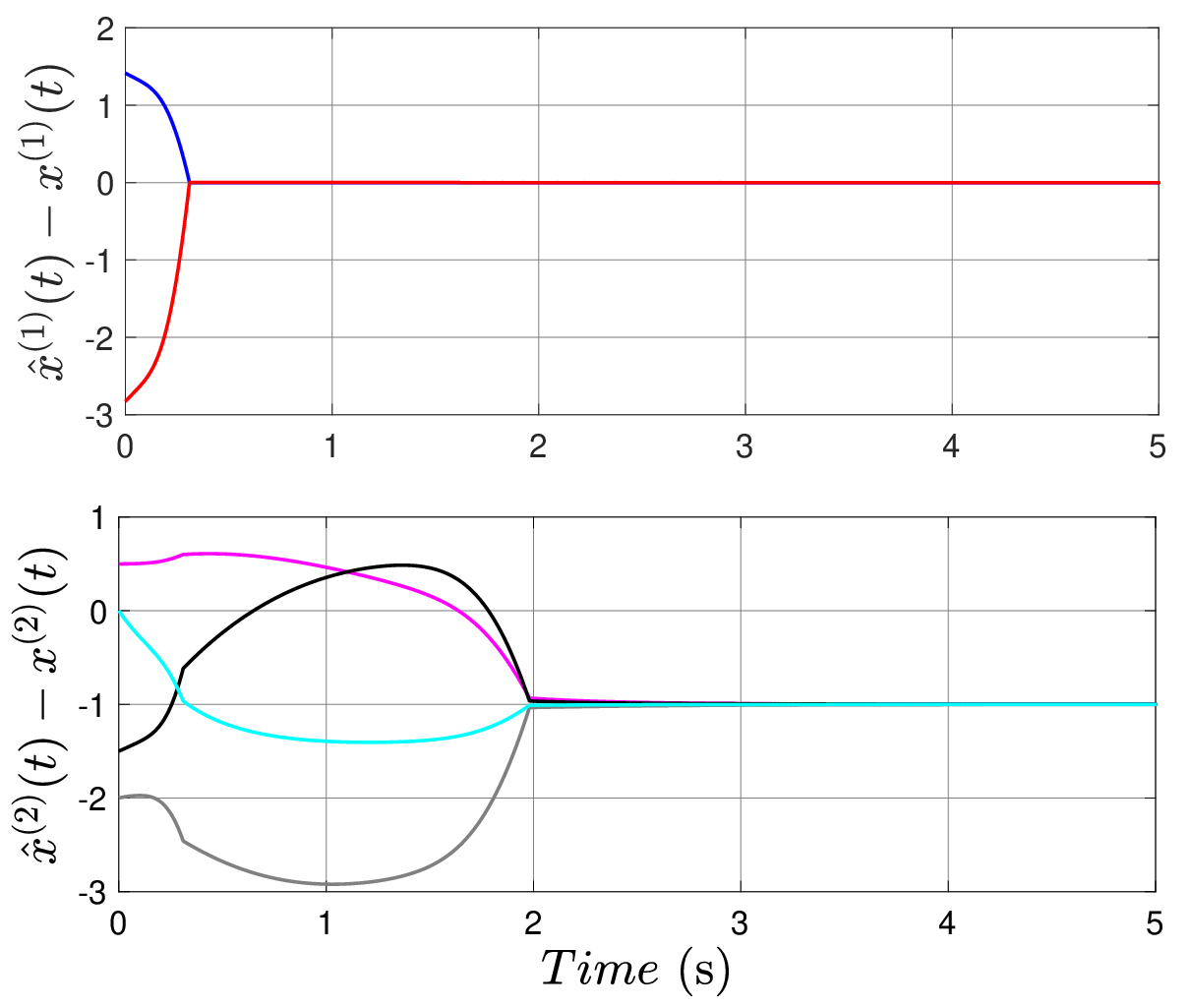
The simulations consider Objective O1 and the state is reconstructed at Node 2. Fig. 1 shows the observation errors for each agent. Recall that Agent 1 estimates two state components and Agent 2 estimates four. As shown in the figure the objective of FCT is achieved with s and s. Notice that the plots of the estimation error for the second agent experiment a jolt at s, when the correct estimation of from the first agent happens.
Fig. 2 depicts the actual trajectories of the state of the system (26), that is, , and its estimates . The latter is reconstructed at Agent 2. As predicted by the theory both sets of trajectories coincide after the FCT at s.

In this appendix we show that, assuming the graph is strongly connected, we can achieve the omniscience Objective O2, implementing a consensus algorithm for each agent and for each partition of the state .
Define as the corresponding portion of the estimated initial condition . Set as the set of neighbour agents transmitting information to the th-agent.
where if and , otherwise. Moreover, if , then , otherwise .
The consensus algorithm can be written also as
and defining as
| (27) |
where , is the standard Laplacian matrix and .
Since the graph is strongly connected and using the Gershgorin theorem we can show that all the eigenvalues of have strictly positive real parts. Moreover, matrix can be always taken to a Jordan normal form. Hence, there exists a proper matrix and a block-diagonal matrix such that
Therefore
The fact that all the eigenvalues of have strictly positive real parts ensures that vanishes.
Thus, the consensus dynamics (27) can be seen as an exponentially stable linear system perturbed by .
However, since converges to zero in finite-time then converges to exponentially.
The estimation of the state at the th agent is finally given by
where .
Actually convergence can be achieved in a fix time using
with and .
Acknowledgments
The first author would like to thank Prof. Nima Monshizadeh for bringing to his attention the concept of Hamiltonian walks and Prof Antonio Pascoal for many insightful remarks about the DSE problem. This paper is partly supported by the Ministry of Education and Science of Russian Federation (14.Z50.31.0031, goszadanie no. 8.8885.2017/8.9), NSFC (61473183, U1509211); and by the Mexican CONACyT Basic Scientific Research grant CB-282807.
References
- [1] S. Aranovskiy, A. Bobtsov, R. Ortega and A. Pyrkin, Performance enhancement of parameter estimators via dynamic regressor extension and mixing, IEEE Trans. Automatic Control, vol. 62, pp. 3546-3550, 2017.
- [2] I. F. Akyildiz, W. Su, Y. Sankarasubramaniam and E. Cayirci, A survey on sensor networks, IEEE Commun. Mag., vol. 40, no. 8, pp. 102-114, 2002.
- [3] J. Bang-Jensen and G. Gutin, Digraphs Theory, Algorithms and Applications, Springer-Verlag, 2007.
- [4] A. Bobtsov, R. Ortega, N. Nikolayev and J. Schiffer, A globally convergent state observer for multimachine power systems with lossy lines, 21st IFAC World Congress, 2020, Berlin, Germany, July 12-17, 2020.
- [5] A. del Nozal, P. Millán, L. Orihuela, A. Seuret and L. Zaccarian, Distributed estimation based on multi-hop subspace decomposition, Automatica, vol. 99, pp. 213-220, 2019.
- [6] W. Han, H. L. Trentelman, Z. Wang and Y. Shen, A simple approach to distributed observer design for linear systems, IEEE Transactions on Automatic Control, vol. 64, no. 1, pp. 329-336, 2019.
- [7] I. Jikuya and I. Hodaka, Kalman canonical decomposition of linear time-varying systems, SIAM Journal on Control and Optimization, vol. 52, no. 1, pp. 274-310, 2014
- [8] T. Kim, H. Shim, and D. D. Cho, Distributed Luenberger observer design, 55th IEEE Conference on Decision and Control, Las Vegas, USA, Dec. 12-14, pp. 6928-6933, 2016.
- [9] G. Kreisselmeier and G. Rietze-Augst, Richness and excitation on an interval—with application to continuous-time adaptive control, IEEE Trans. Automatic Control, vol. 35, no. 2, pp. 165-171, 1990.
- [10] A. Mitra and S. Sundaram, Distributed observers for LTI systems, IEEE Trans. Automatic Control, vol. 63. no. 11, pp. 3689-3704, 2018.
- [11] R. Ortega, A. Bobtsov, A. Pyrkin and A. Aranovskyi, A parameter estimation approach to state observation of nonlinear systems, Systems and Control Letters, vol. 85, pp. 84-94, 2015.
- [12] R. Ortega, L Praly, S. Aranovskiy, B Yi and W. Zhang, On dynamic regressor extension and mixing parameter estimators: two Luenberger observers interpretations, Automatica, vol. 95, pp. 548-551, 2018.
- [13] R. Ortega, V. Gromov, E. Nuño, A. Pyrkin and J. Romero, Parameter estimation of nonlinearly parameterized regressions: application to system identification and adaptive control, 21st IFAC World Congress, Berlin, Germany, July 12-17, 2020. (To appear in Automatica).
- [14] S. Park and N. C. Martins, Design of distributed LTI observers for state omniscience, IEEE Transactions on Automatic Control, vol. 62, no. 2, pp. 561-576, 2017.
- [15] F.F.C. Rego, A.M. Pascoal, A. Aguiar and C.N. Jones, Distributed state estimation for discrete-time linear time invariant systems: A survey, Annual Reviews in Control, https://doi.org/10.1016/j.arcontrol.2019.08.003, 2019.
- [16] W.J. Rugh, Linear Systems Theory, 2nd Edition, Prentice hall, NJ, 1996.
- [17] S. Sastry and M. Bodson, Adaptive Control: Stability, Convergence and Robustness, Prentice-Hall, New Jersey, 1989.
- [18] H. Silm, R. Ushirobira, D. Efimov, J-P. Richard and W. Michiels, A note on distributed finite-time observers, IEEE Transactions on Automatic Control, vol. 64, no. 2, pp. 759-766, 2019.
- [19] H. Silm, R. Ushirobira, D. Efimov, W. Michiels and J-P. Richard, Design of a distributed finite-time observer using observability decompositions, 18th European Control Conference, Naples, Italy, June 25-28, pp. 1816-1821, 2019.
- [20] H Silm, D. Efimov, W. Michiels, R. Ushirobira and J-P. Richard. A simple finite-time distributed observer design for linear time-invariant systems, Systems and Control Letters, Elsevier, In press. hal-02613378.
- [21] L. Wang, J. Liu, and A. S. Morse, A distributed observer for a continuous-time linear system, American Control Conference, Philadelphia, PA, USA, July 10-12, 2019.