SN2019dge: a Helium-rich Ultra-Stripped Envelope Supernova astropy (Astropy Collaboration et al. 2013), corner (Foreman-Mackey 2016), CIGALE (Boquien et al. 2019), emcee (Foreman-Mackey et al. 2013), LAMBDAR (Wright2016a), Lpipe (Perley2019lpipe), matplotlib (Hunter 2007), pandas (McKinney 2010), pyneb (Luridiana et al. 2013), pyraf-dbsp (Bellm & Sesar 2016), scipy (Jones et al. 2001–), simsurvey (Feindt et al. 2019), sncosmo (Barbary et al. 2016) ztfquery (Rigault2018)
Abstract
We present observations of ZTF18abfcmjw (SN2019dge), a helium-rich supernova with a fast-evolving light curve indicating an extremely low ejecta mass () and low kinetic energy (). Early-time (4 d after explosion) photometry reveal evidence of shock cooling from an extended helium-rich envelope of located at from the progenitor. Early-time He II line emission and subsequent spectra show signatures of interaction with helium-rich circumstellar material, which extends from to . We interpret SN2019dge as a helium-rich supernova from an ultra-stripped progenitor, which originates from a close binary system consisting of a mass-losing helium star and a low-mass main sequence star or a compact object (i.e., a white dwarf, a neutron star, or a black hole). We infer that the local volumetric birth rate of 19dge-like ultra-stripped SNe is in the range of 1400–8200 (i.e., 2–12% of core-collapse supernova rate). This can be compared to the observed coalescence rate of compact neutron star binaries that are not formed by dynamical capture.
Keywords:
supernovae: general – supernovae: individual (SN2019dge, iPTF14gqr) – stars: neutronI Introduction
Type Ibc supernovae (SNe Ibc) are believed to be explosions of massive stars that have lost their hydrogen envelopes (Filippenko 1997; Gal-Yam 2017). Their typical rise times ( in the range of 10–25 d) and peak luminosities ( between and mag) suggest ejecta masses () of 1–5 and 56Ni masses () of 0.1–0.4 (Drout et al. 2011; Taddia2018; Prentice2019). The relatively low and high rates of SNe Ibc are not compatible with prediction from the evolution of single massive stars, whose mass-loss rates are not high enough to strip most of the outer layers (Smith2011; Lyman et al. 2016). In contrast, Wolf-Rayet (WR) or helium star descendants of massive stars in close binary systems are thought to be the dominant progenitors for the SN Ibc population (Dessart et al. 2012; Eldridge et al. 2013).
SNe Ibc with the lowest arise from core-collapse of a stellar core with a small envelope. This can occur in tight binaries where a helium star transfers mass to a companion that is small in size. Such a scenario was invoked by Nomoto et al. 1994 as one way to explain the fast evolution of the Type Ic SN1994I with a carbon-oxygen progenitor star of and . Should the degree of stripping be even more extreme, we may expect the so-called ultra-stripped envelope SNe where and are on the order of and , respectively (Tauris2013; Tauris2015; Suwa2015). These weak explosions are one of the two channels to form double neutron star (DNS) binaries that are compact enough to merge within a Hubble time due to gravitational wave (GW) radiation (Tauris2017)11 1 The other channel to form compact DNSs is dynamical capture in a dense stellar environment such as a globular cluster (East & Pretorius 2012; Andrews & Mandel 2019).. Ultra-stripped SNe are therefore a promising progenitor channel of multi-messenger sources that can be jointly studied by the LIGO/VIRGO network and electromagnetic efforts (Abbott et al. 2017a; Abbott et al. 2017b; Goldstein et al. 2017; Coulter et al. 2017; Hallinan et al. 2017; Kasliwal et al. 2017).
Compared with canonical SNe Ibc, we expect light curves of ultra-stripped SNe to be rapidly evolving and subluminous due to the small amount of and produced. Among the group of faint and fast objects, SN2005ek (Drout et al. 2013), SN2010X (Kasliwal et al. 2010), as well as some of the calcium-rich gap transients such as PTF10iuv (Kasliwal et al. 2012), iPTF16hgs (De et al. 2018a), and SN2019ehk (Nakaoka et al. 2020) have been suggested to be good candidates for ultra-stripped SNe (Moriya et al. 2017). However, properties of these objects are also consistent with alternative interpretations, including core-collapse of stars with extended hydrogen-free envelopes (Kleiser & Kasen 2014; Kleiser et al. 2018a; Kleiser et al. 2018b), and explosive detonation of a helium shell on the surface of white dwarfs (Shen2010; Sim2012; Polin2019; De et al. 2020a; Jacobson-Galán et al. 2020).
The most convincing ultra-stripped event to date is the Type Ic SN iPTF14gqr (De et al. 2018b). Its radioactivity-powered emission reveals and , whereas the detection of early-time shock cooling signatures shows that the progenitor is an extended massive star instead of a white dwarf, and therefore pins down its core-collapse origin. Discovered within one day of explosion, iPTF14gqr also demonstrated the importance of early-time observations in securely identifying ultra-stripped SNe.
Here we report the discovery, observations and modeling of the rapidly rising ( d) subluminous ( mag) helium-rich event ZTF18abfcmjw (SN2019dge) discovered by the Zwicky Transient Facility (ZTF; Bellm et al. 2019a; Graham et al. 2019). SN2019dge is consistent with being a helium-rich ultra-stripped SN. Section II describes the discovery and follow up observations. Section III outlines the basic properties of the explosion and its host galaxy. Section IV shows modeling of this transient. Section V provides a discussion on the progenitor system, and Section VI presents the estimated volumetric rates of 19dge-like ultra-stripped SNe. Section VII gives a conclusion of this paper. Calculations in this paper assume a CDM cosmology with , and (Komatsu et al. 2011). All spectra and photometry will be made available by the WISeREP repository (Yaron2012) following publication.
II Observations
II.1 Discovery
SN2019dge was discovered by ZTF, which runs on the Palomar Oschin Schmidt 48-inch (P48) telescope (Dekany et al. 2020). The first real-time alert (Patterson2019) was generated on 2019 Apr 7 10:18:46 (JD ) for a -band detection at mag and J2000 coordinates , . On Apr 8, a new alert was flagged by a science program filter on the GROWTH Marshal (Kasliwal et al. 2019) that is designed to look for fast evolving transients.
II.2 Follow-up Observations
II.2.1 HST Observation
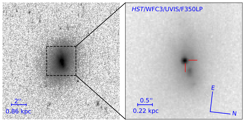
Hubble Space Telescope (HST) observations were obtained as part of our HST “Rolling Snapshots” pilot experiment (GO-15675, Fruchter 2018). This new observational approach requires the PI to update a list of objects of interest each week before the schedule is built, giving the scheduler flexibility to choose a possible source for snapshots. Under this program, we obtained a NUV spectrum using the WFC3 G280 grism, a short (60 s) direct image of this field in the F300X filter to set the wavelength scale of the spectrum, as well as a longer exposure (200 s) in the F350LP filter. The image in the F350LP filter is shown in Figure 1. It has very similar throughput to the zeroth order of the G280 grism.
SN2019dge resides in a compact galaxy SDSS J173646.73+503252.3. From our follow up spectra (see Section III.2), we measure a host redshift of , corresponding to a luminosity distance of Mpc. Figure 1 shows that there is a surface brightness peak to the northwest of SN2019dge ( kpc away), which might trace a star-forming region.
II.2.2 Optical Photometry
Following Yao2019, we perform forced PSF photometry on ZTF difference images generated with the ZTF real-time reduction and image subtraction pipeline (Masci et al. 2019). ZTF image subtraction is based on the Zackay2016 image subtraction method. The sky region of SN2019dge is covered by two ZTF fields with “fieldid” (i.e., ZTF field identifier) 763 and 1799. We exclude all data in field 1799 since the reference image was constructed using images obtained between 2018 May 25 and 2019 Jul 12, which is after the explosion of the transient. Although the ZTF name of this object (ZTF18abfcmjw) may indicate that the transient was discovered in 2018, this is due to an alert generated on 2018 Jul 7 from a candidate detection in negative subtraction (reference minus science) in field 763. We note that the seeing during that night was , larger than 99% of Palomar nights. The irregularly-shaped PSF might cause over-subtraction around the galaxy nucleus in the difference imaging process.
Since field 763 was included in both the Northern sky survey with two epochs (one epoch each in and ) per three nights and the extragalactic high-cadence survey with six epochs (three epochs each in and ) per night (see Bellm et al. 2019b for the design of ZTF experiments), SN2019dge was visited multiple times every night. Therefore, single-night flux measurements in the same filter are binned (by taking the inverse variance-weighted average). This gives a pre-explosion -band limit of 18.95 mag (5 limit computed at the expected position of the transient) on Apr 4 10:36:34. We convert 5 detections to AB magnitudes for further analysis.
Following the discovery of SN2019dge, we obtained follow-up photometry in with an optical imager (IO:O) on the Liverpool Telescope (LT; Steele2004). Digital image subtraction and photometry for LT imaging was performed using the Fremling Automated Pipeline (FPipe; Fremling et al. 2016). Fpipe performs calibration and host subtraction against Sloan Digital Sky Survey reference images and catalogs (SDSS, Alam et al. 2015).
LT and P48 photometry are shown in Figure 2. Absolute and apparent magnitudes are corrected for Galactic extinction mag (Schlafly2011). We assume , and adopt the reddening law from Cardelli et al. 1989. We do not correct for host-galaxy contamination given the absence of Na I D absorption in all spectra at the host redshift. To estimate the epoch of maximum light, we interpolated the - and -band photometry with three-order polynomial functions, as shown in the inset of Figure 2. The time window used in the fit is from to . SN2019dge was found to peak at mag on , and mag on . Hereafter we use phase () to denote time with respect to the -band maximum light epoch, .
We obtained one epoch of late-time imaging with the Wafer Scale Imager for Prime (WASP) mounted on the Palomar 200-inch telescope at d. The data were obtained in band with a total exposure time of 900 s divided into dithered exposures of 300 s each. The data were reduced using standard techniques as described in De et al. 2020b. Image subtraction was performed using archival reference images from the Dark Energy Legacy Survey (Dey et al. 2019), using the method described in De et al. 2020a. The median 5 limiting magnitude of the image is mag. However, the depth at the transient location is limited by the noise from the bright host galaxy, and the transient was not detected to a 5 limiting magnitude of mag.
We also performed forced photometry on archival PTF/iPTF difference images spanning 2009 May 07 to 2016 Jun 13 (Law et al. 2009; Rau2009). No historical detection was found.
| Start Time | Instrument | Phase | Exposure Time | Airmass | Resolution (FWHM) | ||
|---|---|---|---|---|---|---|---|
| (UTC) | (day) | (s) | (Å) | ||||
| 2019 Apr 09 03:30:28 | LT+SPRAT | 500 | 1.80 | 18 | |||
| 2019 Apr 10 03:06:10 | LT+SPRAT | 500 | 1.80 | 18 | |||
| 2019 Apr 10 14:21:44 | Keck1+LRIS | 300 | 1.17 | 6 | |||
| 2019 Apr 22 05:08:00 | HST+WFC3+UVIS | 2250 | — | 43 | |||
| 2019 Apr 24 11:06:43 | P200+DBSP | 1200 | 1.05 | 3–5 | |||
| 2019 Jul 04 11:49:18 | Keck1+LRIS | 1740 | 1.42 | 6 | |||
| 2019 Aug 31 08:04:58 | Keck1+LRIS | 1150 | 1.41 | 6 | |||
| 2019 Sep 28 08:14:27 | Keck1+LRIS | 600 | 2.17 | 6 | |||
| 2020 Feb 18 15:23:40 | Keck1+LRIS | 1450 | 1.38 | 6 |
Note. — Phase is measured relative to -band maximum ().
II.2.3 Swift Observation
Observations with the Neil Gehrels Swift Observatory (Swift; Gehrels et al. 2004) was triggered on Apr 9 and Apr 10. Ultraviolet/Optical Telescope (UVOT; Roming2005) data were obtained in the , , , , , and filters.
UVOT data are reduced using HEAsoft (HEASARC 2014) version 6.17 with a circular aperture. To remove host-galaxy contribution at the location of the SN, we obtained a final epoch in all broad-band filters on 2019 Jun 23 and measured the photometry with the same aperture used for the transient. We present a table of our optical and UV photometry in A.
In parallel with the UVOT observations, Swift observed SN2019dge with its X-ray telescope (XRT; Burrows et al. 2005) between 0.3 and 10 keV in the photon counting mode. We note that no point sources were detected in the XRT event files with . The 3 limits (in count s-1) in the Apr 9, Apr 10, and Jun 23 observations are , , and , respectively. To convert the upper limit count-rate to flux, we adopted the Galactic neutral-hydrogen column density of towards SN2019dge (Willingale2013) and a power-law spectrum in the form of , where has the unit of . Using the PIMMS web tool22 2 https://heasarc.gsfc.nasa.gov/cgi-bin/Tools/w3pimms/w3pimms.pl, we obtained unabsorbed flux upper limits in the 0.3–10 keV band of 5.22, 3.88, and 4.08 , corresponding to luminosities of 5.37, 4.00, and 4.20 . We note that these limits are shallower than X-ray luminosities expected to be seen in SNe (OfekXray2013).
II.2.4 Radio Follow-up
Shortly after the discovery of SN2019dge, we initiated radio follow-up observations in order to constrain the presence of a radio counterpart, as potentially expected in some rapid-rising transients with circumstellar interaction (Weiler2007; Horesh et al. 2013; Ho et al. 2019a). We observed at high frequency radio bands using the Submillimeter Array (SMA, Ho et al. 2004) on UT 2019 Apr 09 between 15:49:17 and 19:51:26 under its target-of-opportunity program. The project ID is 2018B-S047 (PI: Anna Ho). We did not detect SN2019dge in the resulting image, and the 3 upper limits are 2.25 mJy at 230 GHz and 8.4 mJy at 345 GHz.
II.2.5 Spectroscopy
We obtained eight optical spectroscopic follow-up observations of SN2019dge from d to d relative to -band peak using the Spectrograph for Rapid Acquisition of Transients (SPRAT; Piascik2014) on the Liverpool Telescope (LT), the Double Spectrograph (DBSP) on the 200-inch Hale telescope (Oke1982), and the Low Resolution Imaging Spectrograph (LRIS) on the Keck-I telescope (Oke1995). To extract the LT spectra, we use the automated SPRAT reduction pipeline, which is a modification of the pipeline for FrodoSpec (Barnsley et al. 2012). The DBSP spectrum was reduced using a PyRAF-based reduction pipeline (Bellm & Sesar 2016). LRIS spectra were reduced and extracted using Lpipe (Perley2019lpipe).
II.3 Host Galaxy Photometry
To obtain archival photometry of the host galaxy, we retrieved images from the Sloan Digital Sky Survey data release (DR9) (SDSS; Ahn et al. 2012), the Panoramic Survey Telescope and Rapid Response System (Pan-STARRS, PS1) DR1 (Flewelling et al. 2016), the Two Micron All Sky Survey (Skrutskie2006a, 2MASS;), and the unWISE images (Lang 2014) from the NEOWISE Reactivation Year-3 (Meisner et al. 2017). We augmented this data set with Swift/UVOT observations that extend our wavelength coverage to the UV. The photometry was extracted with the software package LAMBDAR (Wright2016a, Lambda Adaptive Multi-Band Deblending Algorithm in R;), to perform consistent photometry on images that are neither pixel nor seeing matched, and tools presented in Schulze et al. (in prep). The UVOT data were reduced in HEAsoft as described in Section II.2.3. The measured host photometry is given in A.
III Properties of the Explosion and its Host Galaxy
III.1 Light Curve Properties
III.1.1 Peak Luminosity, Rise and Decline Timescale
The - and -band peak luminosity of SN2019dge ( mag) is around the lower limit of stripped envelope SNe (Drout et al. 2011; Taddia2018; Prentice2019), and akin to those of the Ca-rich gap transients, which occupy the luminosity ‘gap’ between novae and SNe (peak absolute magnitude to mag, Kasliwal et al. 2012).
To characterize the rise and decline timescales of SN2019dge, following Ho et al. 2020, we calculate rise time () defined by how long it takes the -band light curve to rise from 0.75 mag below peak to peak, and decline time () determined by how long it takes to decline from peak by 0.75 mag (corresponding to half of maximum flux). Since SN2019dge shows no evidence of hydrogen (Section III.2) and exhibits a fast rise (Figure 2), we compare the , , and peak absolute magnitude between SN2019dge and two other groups of transients:
- •
Fast-evolving hydrogen-deficient transients that are fainter than normal SNe Ia (i.e. mag), including SN2002bj (Poznanski2010), SN2005ek (Drout et al. 2013), PTF09dav (Sullivan2011), SN2010X (Kasliwal et al. 2010), PTF10iuv (Kasliwal et al. 2012), iPTF14gqr (De et al. 2018b), iPTF16hgs (De et al. 2018a), SN2018kzr (McBrien et al. 2019), and SN2019bkc (Chen et al. 2020).
- •
“Fast evolving luminous transients” (FELT, Rest2018) or “fast blue optical transients” (FBOT, Margutti et al. 2019). We select well-studied representative objects of this population, including KSN2015K (Rest2018), iPTF16asu (Whitesides2017), AT2018cow (Prentice2018; Perley2019), SN2018gep (Ho et al. 2019b), and ZTF18abvkwla (also known as the Koala; Ho et al. 2020).
In Figure 3, peak magnitudes are given in (observer-frame) -band, except for KSN2015K where we only have observations in the Kepler “white” filter, and iPTF16asu where the rise was only caught in band. We only correct for Galactic extinction to compute (assuming no host extinction). Note that iPTF14gqr and iPTF16hgs are SNe exhibiting double peaked light curves. Since the rise to first peak was not captured, an upper limit of is calculated by taking the time difference between the first -band detection and the latest pre-discovery non-detection33 3 For the second peak, d for iPTF14gqr and d for iPTF16hgs., and absolute magnitude of the first -band detection is considered to be a fainter limit of (plotted in the upper panel). In the lower panel, since observations of iPTF14gqr do not extend to 0.75 mag below its second peak, we present a lower limit of its .
It is clear from the upper panel of Figure 3 that SN2019dge rose faster than normal Ca-rich events such as PTF09dav and PTF10iuv. The of d is similar to the population of FELTs/FBOTs, but SN2019dge is substantially fainter. In the subluminous regime, iPTF14gqr has comparable to SN2019dge, and its first peak has been postulated to be caused by the diffusion of shock-deposited energy out of an envelope around the progenitor star (De et al. 2018b).
The bottom panel of Figure 3 shows that of SN2019dge is longer than that for the most rapid-fading SNe Ibc, such as SN2005ek, SN2018kzr, and SN2019bkc. Its decay timescale is more similar to SN2002bj, SN2010X, the population of Ca-rich transients (PTF09dav, PTF10iuv, iPTF16hgs), and likely iPTF14gqr. It has been suggested that the latter group of events have radioactivity powered main peak with low mass of nickel ().
III.1.2 Bolometric Evolution
We constructed the bolometric light curve at epochs where at least detections in two filters are available by fitting the spectral energy distribution (SED) with a blackbody function (see details of model fitting in Appendix B.1). We plot the physical evolution of SN2019dge with comparisons to iPTF14gqr and iPTF16hgs in Figure 4, where we have adopted the explosion epoch of iPTF14gqr, iPTF16hgs, and SN2019dge estimated by De et al. 2018b, De et al. 2018a, and Section IV.1 of this paper, respectively. The bolometric luminosity of SN2019dge reaches at d after the explosion epoch. The subsequent decline displays an initial fast drop of at age 2–9 d, and transitions to a slower drop of at age 10–30 d.
The bolometric temperature of SN2019dge reaches as high as K at age d and rapidly falls afterwards. The maximum is much hotter than that observed in normal SNe Ibc (6000–10000 K, Taddia2018). Its early light curve evolution is slower than iPTF14gqr, but similar to iPTF16hgs and several other stripped envelope SNe displaying double-peaked light curves (e.g., see Figure 2 of Fremling et al. 2019a). Their first peaks have been modelled by cooling emission from an extended envelope around the progenitor after the core-collapse SN (CCSN) shock breaks out (Modjaz et al. 2019). After d past explosion, flattens to K, similar to the behavior of normal SNe Ibc at a much later phase ( d after explosion, Taddia2018).
Assuming that the photospheric radius can be approximated by and linearly expands at early phase, we fit a linear function to the first few vs. time measurements of SN2019dge which gives . The radius then remains flat at during age 8–30 d, and even appears to slowly recede. The reason for this is that the temperature drops to a recombination temperature for helium and the opacity becomes small. As a result, the outer layers of SN ejecta becomes more transparent, and deeper regions of the ejecta are being probed (Piro2014).
III.1.3 Color Evolution
We compare the color curves of other fast transients to that of SN2019dge in Figure 5, in corresponding pairs of // and // colors. For the double-peaked events iPTF14gqr and iPTF16hgs, “maximum” time corresponds to epoch of maximum light in the second peak.
The early-time blue color of SN2019dge arises from the high-temperature peak. Among other events, SN2002bj, iPTF14gqr and iPTF16hgs exhibit early colors as blue as SN2019dge. Subsequently, SN2019dge displays a color starting out blue and turning redder with time, consistent with a cooling process.
One unusual feature of SN2019dge is that at –9 d after maximum light, the color becomes bluer by mag, while after that the color continues to redden. We notice that iPTF14gqr exhibits a similar trend — around 4 d before the second peak, its color stays flat before getting redder afterwards, while around 2 d before the second peak, its color also turns bluer by mag.
III.2 Spectroscopic Properties
| Transition | d | d | d |
|---|---|---|---|
| He II | — | — | |
| He I | |||
| He I | — | ||
| He I | — | ||
| H | |||
| [S II] | |||
| [S II] | |||
| [O I] | — |
III.2.1 Early Spectral Evolution
The very early spectra at , , and d show a blue continuum and strong galaxy emission lines from the underlying H II region (see Figure 6). In addition, these spectra also show prominent He I and high-ionization He II narrow emission lines. We computed the equivalent width (EW) of He II emission using the spectral line and continuum wavelength ranges given by Khazov et al. 2016. The EW is found to be Å, Å, and Å in the d, d, and d spectra.
In Table 2, we show the measured full width at half-maximum intensity (FWHM) velocities of some emission lines by fitting a Gaussian to the line profile. Since the [S II] , 6731 doublet is definitely from the host galaxy, their line widths serve as a practical measurement of instrumental line-broadening. As shown in column 2, FWHM velocities of the He II and He I emission lines are and , much broader than the resolution of , whereas H is not well resolved. Thus, we infer that the hydrogen emission is from the host galaxy, while the helium lines are from photoionized material exterior to the SN.
III.2.2 Photospheric Phase Spectral Evolution
Broad transient features are present in the and d spectra (Figure 7). These spectra are taken at the photospheric phase where emission comes from a photosphere receding (in mass coordinates) back through freely expanding SN ejecta. The HST spectrum contains little host-galaxy contamination due to its high angular resolution. Prominent galaxy emission lines in the DBSP spectrum are identified and plotted in light red to emphasize transient features. The existence of the P-Cygni He I profile and non-existence of hydrogen nominally classify SN2019dge as a Type Ib SN. We measure the velocity of the He I line by fitting a parabola to the absorption minimum. The resulting fits give velocities of and for the d and d spectra, respectively. This is lower than velocities of normal SNe Ib measured from the He I absorption minimum (, Liu et al. 2016), but higher than that in Type Ibn SNe (, Hosseinzadeh et al. 2017).
In Figure 8, we compare the photospheric phase optical spectra of SN2019dge with other helium-rich events. Note that the DBSP spectrum has host emission lines masked. SN2019dge is different from normal helium-rich stripped envelope SNe Ib/IIb or SNe Ibn in the sense that its P-Cygni absorption minimum in the He I line is weaker. The feature at is often attributed to He I and Fe II triplet , 5018, and 5169 (Liu et al. 2016). The shape of this feature in SN2019dge is similar to those in normal SNe Ib/IIb at much later phases ( d post maximum), indicating that the spectral evolution of SN2019dge is faster. The complex absorption profile at has been identified as a blend of Fe II, Mg II and He I (Hamuy et al. 2002). In the DBSP spectrum, we detected O I and broad Ca II at (due to the 8498, 8542, and 8662 triplet) with clear P-Cygni profiles; Both are major features of stripped envelope SNe (Gal-Yam 2017).
In Figure 9, we compare the HST NUV spectrum with spectra of other types of SNe. The UV part of SN2019dge is much weaker than a blackbody extrapolation of the optical spectra would predict. This has also been seen in normal thermonuclear and CCSNe, and interpreted as strong metal-line blanketing caused by iron-peak elements, particularly Fe II and Co II (Gal-Yam et al. 2008). SN2019dge bears a close resemblance to SN1993J between 2000 Åand 4000 Å. In Figure 9, we also marked the rest wavelength of Mg I and Mg II , 2803. The emission features at in SN2019dge and Gaia16apd are similar to the bump at in SN1993J, which was found to be a NLTE Mg II emission line (Jeffery et al. 1994). This resonance line is blueshifted from its rest wavelength, and is suggested to come from a circumstellar region that is distinctly separated from the SN photosphere in velocity and excitation conditions (Panagia1980; Fransson et al. 1984).
III.2.3 Late-time Spectral Evolution
Figure 10 shows late time spectra of SN2019dge obtained at , , , and d. The general shape of the spectra is determined by the host galaxy, while possible SN features are marked by the dashed lines. The right panels (b), (c), and (d) highlight emission lines at wavelengths of He I, [O I], and [Ca II]. In panel (c) of Figure 10, the [O I] feature consists of two narrow emission peaks. This doublet transitions share the same upper level (–). The observed intensity ratio agrees with the nebular condition, as one would expect in the optically thin regime (Leibundgut et al. 1991; Li & McCray 1992). In panel (d), we mark the position of the [Ca II] doublet in dashed lines, but only the line is clearly detected. It presents a double-peaked profile with a peak separation of .
From panel (a) of Figure 10, it is also clear that in the d spectrum, the He I and [Ca II] lines have broader emission components with Lorentzian profiles at the bases of the narrow emission lines. These Lorentz-shape components are not visible in the d spectrum. Therefore, to further investigate the broader features, we subtract the d spectrum from the d spectrum. The resulting subtraction (Figure 11) reveals intermediate-width (FWHM ) components of He I, [Ca II], and the Ca II IR triplet. It shares a close resemblance to some Type Ibn SNe, such as SN2011hw (Pastorello2015) and SN2015G (Shivvers2017). These intermediate-width features are too narrow to be explained by emission from SN ejecta. Instead, they are probably emitted by a cold dense CSM shell formed by radiative cooling from the post-shock material, as has been proposed to be the case in interacting Type IIn/Ibn SNe (Chugai & Danziger 1994; Smith2017).
Table 2 (column 3 and 4) gives the measured FWHM velocities of narrow emissions shown in panel (b), (c), and (d) of Figure 10. It can be seen that the measured FWHM of other emission lines are similar to the [S II] line-width. Therefore, we conclude that the observed narrow emissions are not resolved.
Due to the low resolution of our LRIS spectra, we cannot directly rule out the possibility that the narrow lines are emanating from the host galaxy. However, there are evidence indicating that they are not merely a background contamination of an underlying H II region:
- (i)
In the d spectrum, the He I and [Ca II] narrow emissions are on top of intermediate-width Lorentzian components characteristic of electron scattering (Huang & Chevalier 2018), which fades away in the d spectrum. However, the hydrogen Balmer lines do not have a broader base in any of our spectra.
- (ii)
The flux intensities of He I, [O I], and [Ca II] lines decrease by a factor of approximately two from d to d, consistent with the temporal evolution from an emission mechanism connected to the aging supernova. As a comparison, the line strengths of the strongest emissions in normal ionized nebulae (H, [O III], [O II], [S II], etc) do not follow this behavior.
- (iii)
Although the He I and [O I] lines labelled in panel (a) of Figure 10 have been observed in H II regions (Peimbert2000; Peimbert2017), the doublet [Ca II] , 7324 has not been detected in gaseous nebulae (Kingdon et al. 1995).
Taken together, we suggest that the narrow components () of He I, [Ca II], [O I] and Ca II are also associated with the transient. Their widths might be consistent with the typical velocities of pre-shock CSM. The detection of these lines at d after the SN explosion suggests that the circumstellar shell extends to ( AU) from the progenitor.44 4 Adopting a conservative shock velocity estimation of , the forward shock travels after 300 d.
III.3 Host Galaxy Properties
We measure properties of the host galaxy using the spectrum obtained at phase d, assuming that the most prominent nebular line emissions of H and [N II] are from the host. The Galactic extinction corrected emission line fluxes of H and [N II] are and , respectively. The fluxes were measured by fitting a Gaussian profile to the emission line profiles, measuring the integrated flux under the profile.
Using the Kennicutt 1998 relation converted to a Chabrier initial mass function (Chabrier 2003; Madau & Dickinson 2014), we infer a star-formation rate of from the H emission line. Note that this is a lower limit since the slit width in the LRIS spectrum is ( kpc at the distance of the host) and the extraction aperture is , whereas the host diameter is about .
We also compute the oxygen abundance using the strong-line metallicity indicator N255 5 N2 log{[N II] /H} (Pettini2004) with the updated calibration reported in Marino et al. 2013. The oxygen abundance in the N2 scale is 8.23 0.01 (stat) 0.05 (sys). We choose not to use the O3N2 index66 6 O3N2 log{([O III] /H)/([N II] /H)} since it requires line flux measurement of H. As can be seen in panel (a) Figure 10, there is substantial stellar absorption around H (4861 Å). Compared to (Asplund et al. 2009), the derived N2 index suggests a significantly subsolar metallicity of (). This estimate places SN2019dge’s host galaxy in the lowest 10% of the distribution of SNe Ibc host galaxy metallicities (Sanders2012), and it is on the lowest 15% in the range of Type Ic-BL SNe host galaxy metallicities (Modjaz et al. 2020)
We determine the stellar mass () of the host galaxy by SED modeling using CIGALE (Boquien et al. 2019). We adopt the stellar population synthesis models from Bruzual & Charlot 2003 with the Kroupa IMF (Kroupa 2001), and assume a double declining exponential star formation history (SFH). In addition, a dust component is added using the Draine & Li 2007 model to account for dust emission. Finally, the total SED model is attenuated by a modified Calzetti extinction law (Calzetti et al. 2000). It assumes that the young stellar population is extincted by the normal Calzetti law, and the old stellar population is extincted less heavily than that by a certain factor ( 1, Charlot & Fall 2000).
The fitted SED is shown in Figure 12. The derived total stellar mass is , the mass of the stars alive is , and the inferred SFR is , about 2.5 times the SFR inferred from the H flux measurement. The host extinction, , is mag and mag for the young and old stellar population, respectively, both of which are insignificant. The stellar mass and the SFR of the this galaxy are in the lower half of the hosts of Type Ibc SN in the PTF sample (Schulze et al. in prep.).
IV Modeling
IV.1 Shock Cooling Powered Fast Rise
Supernovae light curves are mainly powered by shock energy or radiative diffusion from a heating source. We first examine if the peak of SN2019dge is likely to be powered by the radioactive decay of 56NiCoFe. With a peak luminosity of and a rise time of –, SN2019dge falls into the unshaded region of Kasen 2017, where an unphysical condition of is required. Therefore, we rule out radioactivity as the power source for the fast rise of the light curve.
There have been clues for the early emission mechanism of SN2019dge,:
- (i)
The fast (Figure 3), high initial high temperature (middle panel of Figure 4), blue color (Figure 5), and relatively fast color evolution of SN2019dge are reminiscent of shock cooling emission (Nakar & Piro 2014; Piro2015).
- (ii)
The color jump in is observed 6–9 d after maximum (left panel of Figure 5). It is roughly at this phase that the change in bolometric luminosity decline rate transitions from 0.36 to 0.11 (upper panel of Figure 4). This supports the idea that the dominant power mechanisms before and after this transition are different.
Therefore, we model the early light curve as cooling emission from shock-heated extended material, which is located at the outer layers of the progenitor or outside of the progenitor. We use models presented by Piro2015 to constrain the mass and radius of the extended material ( and , respectively), where includes only mass concentrated around . This model is built on analytical results of Nakar & Piro 2014. Details of the model fitting to multi-band observations are illustrated in Appendix B.2.
In Figure 13, the bolometric light curve measured in Section III.1 is shown in black. We also show late-time -band measurements in grey empty circles as a proxy of bolometric light curve evolution. The dashed green line shows the best-fit model of , cm (i.e., ), and explosion epoch at phase d (i.e., the explosion occurred 0.45 d before the first detection in -band). The amount of energy in the extended material is well constrained to be .
Given the simple assumptions of the model, we expect the constraints on and to be only approximately accurate. We thus conclude that the early shock cooling emission was produced by an extended envelope with a mass of locating at a radius of (). There are now numerous cases of early cooling envelope emission observed in CCSNe, where the extended material is estimated to have lower mass (–) and larger radius () compared to SN2019dge (Modjaz et al. 2019).
IV.2 Mass-Loss Estimate from He II
Early-time low-velocity He II emission (Section III.2.1) has been detected in nearly twenty hydrogen-rich CCSNe and one hydrogen-poor SN iPTF14gqr. This feature often fades away within a few hours to a few days after the explosion (Yaron2017). The high ionization potential of this line requires high temperature or an ionizing flux, which might come from either shock breakout or CSM interaction (Gal-Yam et al. 2014; Smith2015). Due to the rapid decrease in at the three epochs of our early-time spectra and the similarity between SN2019dge and iPTF14gqr, we favor shock cooling emission as the origin of recombination helium lines. Therefore, we can use the luminosity of the He II line to make an order-of-magnitude estimate on properties of the emission material, following the procedure given by Ofek et al. 2013a and De et al. 2018b.
Assuming that the immediate CSM around the progenitor has a spherical wind-density profile of the form , where is distance from the progenitor, is the wind density parameter, is the wind velocity, and is the mass-loss rate. The integrated mass of the emitting material from to is
| (1) |
where is assumed to be of order unity.
We can relate the mass of the He II region to the He II line luminosity using
| (2) |
Here
| (3) |
(in ) is the emission coefficient for the transition. is mass of a helium nucleus, is the number density of doubly ionized helium and is the number density of electrons.
Assuming a temperature of K, electron density of , and Case B recombination, we get (Storey1995). Using and the density profile, Eq. (2) can be written as
| (4) |
The location of the emitting region can be constrained by requiring that the Thompson optical depth () in the region must be small for the lines to escape. We require
| (5) |
Thus
| (6a) | ||||
| (6b) | ||||
The d emission line flux is measured to be , corresponding to . Hence, we get , , and . Adopting a wind velocity of as measured from the He II FWHM, the mass-loss rate can be constrained to be . Note that these estimates can be affected if the CSM cannot be well characterized by a spherically symmetric density profile, or if the emitting region was confined to a thin shell ().
IV.3 Constraints from Radio Upper Limits
Radio emission in SNe is produced by shock accelerated electrons in the circumstellar material as they gyrate in the post-shock magnetic field when the shock freely expands. Should the circumstellar medium be formed by a pre-SN stellar wind, the radio synchrotron radiation can be used to probe the pre-explosion mass-loss (Chevalier 1982). High frequency ( GHz) bright () radio sources are often found to be associated with gamma-ray bursts (GRBs), TDEs, and relativistic transients (see Figure 6 of Ho et al. 2019a). Among normal SNe Ibc, moderate submillimeter luminosity at has been observed in SN1993J (Weiler2007) and SN2011dh (Horesh et al. 2013).
Our SMA observations constrain the submillimeter luminosity of SN2019dge to and . We place these upper limits in physical context using the synchrotron self-absorption model given by Chevalier 1998. The expected radio luminosities are computed at 230 and 345 GHz for two types of circumstellar environments — one with a wind-density with the same parameterization as that adopted in Section IV.2 and the other with a constant-density environment ().
Adopting the explosion epoch found in Section IV.1, our SMA observations were obtained at 2.75 d after explosion. Given the early time of these observations, we consider constant shock velocities at 0.1–0.25, as found to be typical in SNe Ibc (Wellons2012). We assume an electron energy power-law index of , a volume filling factor , and that the electrons and magnetic field in the post-shock region share constant fractions of the post-shock energy density, i.e., .
The expected radio luminosity predicted by the Chevalier model in the two environments at 230 GHz are shown in Figure 14 by the color maps, and the black contours indicate our limits. As can be seen, only small regions have expected luminosity higher than the limits (indicated by the hatched regions), and thus our observations are not deep enough to provide stringent constrains on the circumstellar properties. Compared with 230 GHz, the parameter space is even more poorly constrained at 350 GHz and are thus not shown.
IV.4 Radioactivity Powered Main Peak
After subtracting the shock cooling emission from the bolometric light curve, the remaining light curve has a peak luminosity of and a rise time of . In the shaded region of Kasen 2017, this falls between the and lines, indicating that the remaining component can be powered by 56Ni decay. Apart from this, the moderate of SN2019dge (bottom panel in Figure 3) is similar to that found in a few Ca-rich transients, and consistent with coming from radioactivity. Here we use two methods to estimate and .
First of all, we use analytical models (Arnett 1982; Valenti2008; Wheeler2015) to constrain the nickel mass (, a characteristic photon diffusion timescale (), and a characteristic -ray escape timescale (). Details of the model fitting are given in Appendix B.3. The dotted blue line in Figure 13 shows the best-fit model of , d, and d. Thus, using Equation (B9), the ejecta mass can be estimated to be
| (7) |
Here we adopt the the mean opacity of SNe Ibc found by Taddia2018. In Section III.2.2, the the photospheric velocity of is measured at phase d (i.e., –16 d post explosion). At that time, Figure 4 shows that stays roughly flat, indicating that a certain amount of ejecta in the outer layers should have a velocity greater than that measured from the He I absorption minimum. Therefore, we adopt the measured from early evolution (see Section III.1.2) to be a more appropriate estimate for . The kinetic energy is then calculated to be
| (8) |
Khatami & Kasen 2019 presented improved analytic relations (compared with the original Arnett 1982 model) between and . When d, (see Equations B5, B6), and hence we have an exponential heating function
| (9) |
where . In this case, KK19 (Eq. 21) shows that the relation between peak time and luminosity is:
| (10) |
where gives a reasonable match to numerical simulations. With and d, we get an estimate of .
can be estimated using Eq. 23 of KK19:
| (11) |
where is the characteristic timescale without any numerical factors
| (12) |
We derive d, which implies
| (13) |
The kinetic energy of the ejecta is then .
In conclusion, the estimates derived from simplified model fitting and new analytic relations from KK19 are roughly the same. The ejecta mass (), the nickel mass (), and the total kinetic energy () of SN2019dge are very small.
V Interpretation
V.1 A Core-Collapse Supernova
At early times, the cooling emission from shock-heated surrounding material of and () corroborates that the progenitor of SN2019dge is a star with an extended envelope. Indeed stellar evolution models predict envelope radii of 10–100 for helium stars with zero-age helium core masses within 2.5–3.2 that have stripped all of the hydrogen-rich envelope (Woosley2019; Laplace et al. 2020). Therefore, the early-time shock cooling light curve serves as strong evidence that SN2019dge is the explosion of a star with inflated radius (not a compact object).
The 56Ni mass of inferred from the radioactivity-powered decay is much greater than that produced in electron-capture SNe (, Moriya et al. 2014), whereas the ejecta velocity of is larger than that expected in fallback SNe (; Moriya et al. 2010). Therefore, we conclude that SN2019dge is associated with the class of Fe CCSNe.
V.2 An Ultra-Stripped Progenitor
As noted in the introduction, the majority of SNe Ibc, with in the range of 1–5 , are believed to come from binary evolution. The small amount of ejecta mass seen in SN2019dge () requires extreme stripping prior to the explosion in a binary system, which suggests an ultra-stripped progenitor (Tauris2013).
Compared with iPTF14gqr, where the second peak of the light curve suggests , SN2019dge has a higher ejecta mass. In particular, the helium-rich photospheric spectra indicate that SN2019dge has a greater amount of helium in the ejecta. He I emission lines are non-thermally excited by collisions with fast electrons, which result from Compton processes with -rays from 56Ni decay (Dessart et al. 2012; Hachinger et al. 2012). On the other hand, the weak absorption strength in the He I P-Cygni profile (Figure 7 and Figure 8) suggests that the helium envelope mass of SN2019dge is substantially lower than that in a canonical Type Ib SN (Fremling et al. 2018). While the stripping in SN2019dge is less extreme than for iPTF14gqr, the striking similarities between these two events indicate that they probably originate from similar channels.
The He II flash ionized emission comes from optically thin material located at (). This is even larger than the expected orbital separation required for extreme stripping. Therefore, material at such a large radius might be ejected prior to the explosion, with a mass-loss timescale . The inferred mass-loss rate of is much higher than that observed in Galactic Wolf-Rayet stars (Smith2014). Additionally, the photospheric and late-time spectra of SN2019dge signify interaction with a helium-rich extended dense shell, which may also consist of gas originally ejected by the progenitor as a stellar wind or deposited by binary interaction. The high mass-loss rate and short ejection timescale can be achieved in the final stages of stellar evolution by several mechanisms: 1. a powerful outflow driven by super-Eddington wave energy deposition during the last few years before explosion (Quataert2012); 2. explosive mass ejection due to violent silicon flashes within a few weeks before the explosion of low-mass helium stars (Woosley2019); 3. nonconservative case BB mass transfer in binary evolution of ultra-stripped stars (Tauris2015).
| Name | ||||||||
|---|---|---|---|---|---|---|---|---|
| () | (d) | () | () | () | () | () | () | |
| iPTF14gqr | 10000 | 0.22 | 8.35 | |||||
| iPTF16hgs | 10000 | 0.78 | 2.29 | |||||
| SN2018lqo | 8250 | 0.63 | 3.08 | |||||
| SN2019dge | 8000 | 0.30 | 1.70 |
V.3 Stellar Evolution Pathways
Here we discuss possible evolution paths of SN2019dge’s progenitor.
We first consider the scenario where SN2019dge comes from a progenitor more massive than in a binary system that loses its mass in case B mass transfer. Yoon2010 showed that subsequent wind mass loss is weak at subsolar metallicity of (similar to the calculated in Section III.3), such that the final mass of the primary at the time of core-collapse will be higher than 3.8 . This will lead to , assuming that the explosion forms a neutron star of 1.5 . This inferred ejecta mass is much higher than that observed (), so this scenario is not favored.
We next consider the possibility that the primary has an initial mass . In many binary scenarios involving a companion that is a main sequence star, the primary will experience stable case B mass transfer that strips the hydrogen envelope, followed by case BB mass transfer that strips most of its helium envelope, resulting in an ultrastripped exploding star. Zapartas2017 performed population synthesis simulations, showing that for the pre-SN helium star to reach , a relatively wide range of companion mass is possible (initial mass 4–10 ). Therefore, this scenario is consistent with observations of SN2019dge. A compact object companion is less likely because its lower mass would likely lead to unstable case B mass transfer, with a post-common envelope orbital separation much smaller than the inferred radius of the progenitor of SN2019dge (Laplace et al. 2020).
The final mass of the helium envelope depends on the initial mass of the helium star and the orbital period of the compact binary. To reconcile with the ejecta mass observed in SN2019dge, we expect a small final envelope mass () but large enough for optical helium features to be observed in the SN explosion (, Hachinger et al. 2012). This can be achieved in a system where the progenitor is a helium star in a compact binary with d at the start of the helium burning phase (Tauris2015). However, the large inferred radius of the progenitor requires an orbital separation , implying an orbital period of tens of days at the time of explosion, depending on the companion mass.
V.4 Comparison with Other Ultra-Stripped SN Candidates
In addition to SN2019dge and iPTF14gqr, we search the literature for other subluminous fast-evolving hydrogen-poor SNe whose light curves can potentially be well fitted by an early-time shock-cooling component from an extended envelope and a radioactivity-powered second peak with small . We recover iPTFF16hgs (De et al. 2018a) and SN2018lqo (De et al. 2020a) as ultra-stripped SN candidates. Here we apply our modeling approach described in Section IV.1 and IV.4 to iPTF16hgs and SN2018lqo to distill the physical parameters of these two events. We show the results in Table 3. The ejecta masses of iPTF16hgs and SN2018lqo are greater than that in SN2019dge and iPTF14gqr by a factor of , and falls inside the range of expected in explosions of a helium star orbiting a compact object, but is at the upper side of the boundaries (Tauris2015).
A full discussion of the progenitors of iPTF16hgs and SN2018lqo is beyond the scope of this paper. Here we refer to a recent study conducted by De et al. 2020a, which classify these two objects into the “green Ca-Ib” subclass in the Ca-rich SNe category. This class of objects is spectroscopically similar to SNe Ib at maximum light, and do not exhibit line-blanketed continua at –5500 Å. De et al. 2020a proposed that pure helium-shell detonations or deflagrations can explain their photometric and spectroscopic properties. Although it has been suggested that the existence of early first peak can distinguish ultra-stripped SNe from other Ca-rich transients arising from helium dotonation on the surface of white dwarfs (Nakaoka et al. 2020), the early-time peak might also be caused by radioactive decay from short-lived isotopes in the outermost ejecta (De et al. 2020a). For example, the double-peaked Ca-rich transient SN2018lqo occurs in an elliptical galaxy, which is not expected to be the host for ultra-stripped SNe.
Although we only include hydrogen-poor events in this comparison, we note that SN2019ehk, a Ca-rich transient that exhibits flash ionized hydrogen in its early-time spectra (Jacobson-Galán et al. 2020) as well as possible hydrogen photospheric features (De et al. 2020a), has also been suggested to be an ultra-stripped CCSN (Nakaoka et al. 2020). If both iPTF16hgs and SN2019ehk are bona fide ultra-stripped SNe, there might exist a continuum of ejecta mass from normal stripped envelope SNe (), to a higher degree of stripping in the progenitors of SN2019ehk and iPTF16hgs (), to a more extreme degree of stripping seen in SN2019dge (), to the most extreme stripping seen in iPTF14gqr (). The remaining amount of helium, the companion mass, and final orbital separation might become smaller along this sequence.
VI Rates
As progenitors of compact neutron star binaries, the volumetric rates of ultra-stripped SNe have implications for our understanding of the evolutionary pathways leading to these systems and the gravitational waves detected by existing and upcoming facilities such as LIGO/VIRGO (Abbott et al. 2017a).
Based on population synthesis calculation, Tauris2015 estimate that the volumetric rates of ultra-stripped SNe should be –1% of the rate of Core-collapse SNe. Using the properties of the promising ultra-stripped SN iPTF14gqr (De et al. 2018b), Hijikawa et al. 2019 estimate the volumetric rates of iPTF14gqr-like ultra-stripped SNe to be , or % of the local CCSNe rate (Li et al. 2011a). However, since existing ultra-stripped SN candidates were found outside of systematic SN classification efforts, observationally constraining the rates of ultra-stripped SNe has not been possible thus far.
VI.1 Simple Estimation
VI.1.1 Using the BTS Sample
SN2019dge was followed up as a part of the ZTF Bright Transient Survey (Fremling et al. 2019b, BTS,) that aims to spectroscopically classify all extragalactic transients in ZTF brighter than 18.5 mag at peak. Since BTS only reads from the ZTF public alert stream (highlighted with a greater marker size in Figure 15), SN2019dge peaks between 18.5 and 19.0 mag in the BTS sample. Thanks to the relatively high spectroscopic completeness (%) at the brightness limit of 19.0 mag, we can directly place constraints on the rates of 19dge-like ultra-stripped SNe using the BTS sample.
SN2019dge peaked at an absolute magnitude of mag in -band. At the BTS peak brightness limit of 19.0 mag, objects similar to SN2019dge would be detectable out to 123 Mpc. Thus, taking only the local 123 Mpc volume within redshift of , we compare the number of CCSNe brighter than 19.0 mag at peak that were found in the BTS experiment in its first 12 months of operations (between 2018-06-01 and 2019-06-01). In this time period, BTS classified a total of 116 CCSNe in this volume. As such, the detection of one object in this sample constrains the rate of ultra-stripped SNe to be 0.86% of the CCSNe rate brighter than mag in this volume.
Taking the observed luminosity function of CCSNe in the local universe (Li et al. 2011b), we find that % of CCSNe are fainter than mag. The luminosity function corrected rate of 19dge-like events is then 0.43% of the local CCSNe rate. The inferred rate is consistent with that estimated in Tauris2015, but higher than that inferred for iPTF14gqr-like events (Hijikawa et al. 2019). Adopting the CCSNe volumetric rate of (Li et al. 2011a), the volumetric rate of 19dge-like ultra-stripped SNe rate is 300 . This rate estimation is only a lower limit, since the fast photometric evolution of objects similar to SN2019dge can be easily missed due to the slower 3-day cadence of the ZTF public survey.
VI.1.2 Using the CLU sample
The ZTF team also conducts a campaign to spectroscopically classify all SNe within 200 Mpc by filtering transients occurring in galaxies with previously known redshifts within in the Census of the Local Universe (CLU) catalog (De et al. 2020a). Hereafter we refer this experiment as CLU. The spectroscopic completeness of transients in the CLU sample that had at least one detection brighter than 20 mag is 89%. Since CLU reads from the whole ZTF alert stream (e.g., all data points shown in Figure 15), the higher-cadence sub-surveys allow it to better characterize fast-evolving SNe. However, the uncertainty in this experiment is the incompleteness of the input galaxy catalog. The redshift completeness fraction (RCF) is % at the lowest redshifts and decreases to % at , as measured by the BTS experiment (Fremling et al. 2019b).
At the CLU peak brightness limit of 20.0 mag, objects similar to SN2019dge would be detectable out to 195 Mpc. Between 2018-06-01 and 2019-06-01, CLU classified a total of 273 CCSNe in this volume, whereas no good ultra-stripped SN candidates have been identified. We place an upper limit of ultra-stripped SNe rate to be 5100 following the simple calculation described in Section VI.1.1. However, it is also susceptible to the fast evolution of 19dge-like SNe being missed by the observation gaps. In Section VI.2 we attempt to place robust estimates of 19dge-like ultra-stripped SNe rate by running simulated surveys with the ZTF cadence.
VI.2 Estimation Based on Survey Simulations
We utilize simsurvey (Feindt et al. 2019), a python package designed for assessing the rates of transient discovery in surveys like ZTF. To simulate the expected yield of a specific type of transient given a volumetric rate, simsurvey requires three inputs: 1) A survey schedule. We use the actual ZTF observing history in - and -band between 2018-06-01 and 2019-06-01 in any of the public or collaboration surveys as the input survey plan. 2) A transient model. We construct a light curve template of SN2019dge (see details in Appendix B.4). Using the template, we generate a TimeSeriesSouce model in the sncosmo package (Barbary et al. 2016). 3) A function to sample the transient model parameters. Transients are injected out to a redshift of , since objects further out are not expected to peak brighter than 20.0 mag.
We examine the expected number of detected 19dge-like SNe for a range of input rates. For each input rate, we performed 300 simulations of the ZTF observing plan. In order to select transient candidates that would have passed the selection criteria of the BTS or CLU experiment and been flagged as an object with photometric properties consistent with being a 19dge-like ultra-stripped SN, we apply cuts on the simulated light curves as described below.
For the BTS filter, we only use public survey pointings, and reject SNe at low Galactic latitudes () to be consistent with the BTS experiment (Fremling et al. 2019b). In either the - or -band light curve, we identify peak light as the brightest detection in the simulated light curve, and require:
- (i)
peak magnitude mag
- (ii)
within 4.1 d before peak, there must be at least one detection or one upper limit deeper than 1.5 mag below peak
- (iii)
within 15 d after peak, there must be at least three detections, and the measured decline rate must be greater than .
Criterion (ii) is set to require that the fast rise of the light curve can be recognized from the observation. This is essential since if we only discover SN2019dge at the radioactive tail, we will probably classify it as a low-velocity SN Ib. Criterion (iii) is made to ensure that the rapid decline of the light curve can be captured, such that the small ejecta mass can be inferred.
For the CLU filter, we use all ZTF pointings, and require that in either the - or -band light curve:
- (i)
peak magnitude mag
- (ii)
the light curve must satisfy at least one of the following criteria: 1) within 4.1 d before peak, there must be at least one detection or one upper limit deeper than 1.5 mag below peak, 2) within 2.5 d before peak, there must be at least one detection deeper than 0.75 mag below peak
- (iii)
same as criterion (iii) applied in the BTS filter.
We apply the above criteria to the actual observations of CCSNe in the BTS and CLU sample. We identify one other SN — ZTF18abwkrbl (SN2018gjx) — that pass our criteria. However, ZTF18abwkrbl is a SN IIb that clearly shows hydrogen in the spectra, and can therefore be excluded as an ultra-stripped SN candidate (Tauris2015).
In Figure 16, we show the number of transients that pass our selection criteria as a function of the input volumetric rate. The solid line and shaded region indicate the mean and 68% credible region of the 300 simulations. In the actual BTS experiment, there was only one detected ultra-stripped SN. Therefore, we consider the range of volumetric rate where one falls within the shaded red region as a constraint on the rate of 19dge-like ultra-stripped SNe. This gives in the range of 1400–28000 .
Using the fact that there were zero ultra-stripped SN detected in the actual CLU experiment, the grey shaded region in Figure 16 might suggest . However, this upper limit needs to be corrected for offset distribution and galaxy catalog incompleteness. First of all, as discussed in De et al. 2020a, the CLU experiment is restricted to transients coincident within 100′′ of the host galaxy nuclei. SN2019dge and iPTF14gqr are 0.5′′ and 24′′ from their host galaxies (all within 100′′). Although a large sample of ultra-stripped SNe is needed to examine the host offset distribution of this class of objects, the fact that they arise from massive binary evolution suggest that the correction due to this factor should be small. Secondly, the incompleteness of the input galaxy catalog possibly leads to an underestimation of ultra-stripped SNe rate by a factor of 55–80%, as indicated by the RCF. We adjust for such an incompleteness by increase the upper limit from 4500 to 8200 .
Combining results from the BTS and CLU experiments, we derive a 19dge-like ultra-stripped SNe rate of 1400–8200 , corresponding to 2–12% of CCSNe rate.
VI.3 Effects of Different Envelope Masses and Radii
Given the low mass of ultra-stripped progenitors, we expect to see shock cooling emission from the inflated pre-explosion star, as has been clearly seen in the case of iPTF14gqr and SN2019dge in the fast early-time evolution and blue colors of the optical light curve. As is shown by Nakar & Piro 2014, rise time of the shock cooling light curve is determined by mass of the extended material , while the peak luminosity is mainly modulated by . We demonstrate this dependence in Figure 17. We simulate shock cooling light curves by varying and , and at the same time setting (the value found in SN2019dge).
In the upper panel, is defined in the same way as in Section III.1.1 (rise time from half-max to max). The rising part of the cooling light curve can be captured by a three-day, two-day, and one-day cadence optical survey at , , and , respectively. Transients with will not pass our selection criteria in Section VI.2. In the bottom panel, we show the expected absolute luminosity at peak of the -band cooling light curve. As is readily shown, for ultra-stripped progenitors with an extended radius , a survey like ZTF is only sensitive to objects in the local universe (–150 Mpc) for the subsequent evolution of the light curve to be well-characterized. Taken together, we conclude that our estimation of the ultra-stripped SNe rate does not include ultra-stripped progenitors with or .
VI.4 Discussion
If the companion of the pre-explosion helium star is a low mass main sequence star, a white dwarf, or a black hole, SN2019dge will not be the progenitor of a double neutron star system, and thus the inferred is not connected with . Even in the case that the companion is a neutron star, if the forming DNS binary has orbital periods more than d, it will not merge within the age of the Universe (Tauris2015). Therefore, the above estimation of the ultra-stripped SNe rate should provide an upper limit to the local coalescence rate density () of double neutron stars not formed via dynamical capture in a globular cluster (East & Pretorius 2012; Andrews & Mandel 2019).
VII Conclusion
In this paper we have presented the discovery, observation and modeling of the transient SN2019dge. We summarize the main characteristics of this object below:
- (a)
Peak absolute magnitudes are mag and mag. In -band, rise time (half-max to max) is 2.0 d and decay time (max to half-max) is 8.6 d. SN2019dge is one of the most rapidly rising subluminous SNe I discovered to date.
- (b)
Early-time spectra show a blue continuum and flash He II features that indicate a high mass-loss rate of .
- (c)
Photospheric spectra indicate helium-rich ejecta, and the prominent NUV Mg II emission suggests interaction between SN ejecta and CSM.
- (d)
Late-time spectra show signatures of interaction with helium-rich CSM, similar to that observed in Type Ibn SNe.
- (e)
SN2019dge exploded in a compact low-metallicity () galaxy with small star formation rate () and stellar mass ().
- (f)
The bolometric light curve of SN2019dge peaks at , and can be explained by a combination of two components. The first component is consistent with shock cooling from an envelope of located at () from the progenitor. The second component is powered by of 56Ni.
- (g)
We estimate the ejecta mass and kinetic energy of SN2019dge to be and , respectively.
We interpret SN2019dge as a helium-rich ultra-stripped envelope SN.
Based on the one event, we estimate the rate density of 19dge-like ultra-stripped SNe (with and ) to be 1400–8200 . This can be compared to the merger rate of DNS systems not formed via dynamical capture. The first detection of gravitational waves from the merging DNS binary GW170817 gave – (Abbott et al. 2017a). Detection of GW190425 provides an update of – (Abbott et al. 2020). Based on an archival search for EM170817-like transients (known as “kilonovae” or “macronovae”) in the PTF database, Kasliwal et al. 2017 reported an upper limit on the rate of , which might be doubled if the typical kilonova is 50% fainter than EM170817.
It is important to compare ultra-stripped SNe rate and constrained by future GW observations. If the former is smaller than the latter, it will provide evidence for the dynamical formation channel to be the major path for forming DNS systems. A better constraint of ultra-stripped SNe rate is also essential in our understanding of the final stages of helium star evolution in binary systems. As such, further systematic searches for ultra-stripped SNe are requried to reduce the large uncertainties of the current estimation. Moving forward, the discovery of ultra-stripped SNe will still rely on high-cadence wide-field experiments such as ZTF. In particular, the upcoming ZTF-II, with a two-day cadence all sky survey, coupled with higher cadence boutique experiments, is well-positioned to carry out this task.
Appendix A UV and Optical Data
| Date (JD) | Instrument | Filter | ||
|---|---|---|---|---|
| 58582.1544 | LTIOO | 18.590 | 0.010 | |
| 58582.1552 | LTIOO | 18.840 | 0.020 | |
| 58582.1575 | LTIOO | 19.110 | 0.020 | |
| 58582.1583 | LTIOO | 19.280 | 0.070 | |
| 58584.2341 | LTIOO | 18.570 | 0.020 | |
| 58580.4421 | P48ZTF | 20.828 | 0.148 | |
| 58580.4842 | P48ZTF | 20.891 | 0.139 | |
| 58582.8289 | SwiftUVOT | 18.606 | 0.193 | |
| 58582.8280 | SwiftUVOT | 18.289 | 0.113 | |
| 58582.8346 | SwiftUVOT | 18.550 | 0.068 | |
| 58582.8261 | SwiftUVOT | 18.685 | 0.108 | |
| 58582.8299 | SwiftUVOT | 18.802 | 0.103 | |
| 58582.8337 | SwiftUVOT | 18.679 | 0.404 |
Note. — and are observed magnitude (without extinction correction) in AB system. A machine-readable table of all 117 photometric data points will be made available online.
| Instrument/Filter | () | ||
|---|---|---|---|
| UVOT/ | 2079.0 | 20.492 | 0.124 |
| UVOT/ | 2255.1 | 20.471 | 0.172 |
| UVOT/ | 2614.2 | 20.081 | 0.155 |
| UVOT/ | 3475.5 | 19.631 | 0.145 |
| UVOT/ | 4359.1 | 18.812 | 0.139 |
| UVOT/ | 5430.1 | 18.194 | 0.171 |
| SDSS/ | 3561.8 | 19.636 | 0.082 |
| SDSS/ | 4718.9 | 18.540 | 0.015 |
| SDSS/ | 6185.2 | 18.056 | 0.026 |
| SDSS/ | 7499.7 | 17.885 | 0.028 |
| SDSS/ | 8961.5 | 17.697 | 0.089 |
| PS1/ | 4866.5 | 18.538 | 0.042 |
| PS1/ | 6214.6 | 18.029 | 0.030 |
| PS1/ | 7544.6 | 17.845 | 0.033 |
| PS1/ | 8679.5 | 17.755 | 0.050 |
| PS1/ | 9633.3 | 17.710 | 0.063 |
| 2MASS/ | 12410.5 | 17.653 | 0.215 |
| 2MASS/ | 16513.7 | 17.690 | 0.420 |
| WISE/ | 34002.6 | 18.460 | 0.069 |
| WISE/ | 46520.1 | 18.953 | 0.136 |
Note. — and are observed magnitude (without extinction correction) in the AB system.
Appendix B Modeling of SN2019dge
| () | ( K) | ||
|---|---|---|---|
| 2.74 | |||
| 1.72 | |||
| 0.69 | |||
| 0.24 | |||
| 1.09 | |||
| 3.26 | |||
| 4.24 | |||
| 5.25 | |||
| 6.83 | |||
| 7.98 | |||
| 8.98 | |||
| 10.05 | |||
| 10.92 | |||
| 11.89 | |||
| 13.06 | |||
| 14.05 | |||
| 14.97 | |||
| 16.09 | |||
| 23.96 | |||
| 27.00 | |||
| 27.98 | |||
| 29.23 | |||
| 33.24 |
| Description | Prior | |
|---|---|---|
| log10 of extented material radius in cm | ||
| log10 of extented material mass in | ||
| explosion epoch in MJD relative to | ||
| SN energy divided by | ||
| divided by |
| Description | Prior | |
|---|---|---|
| characteristic photon diffusion time in day | ||
| log10 of nickel mass in | ||
| characteristic -ray escape time in day |
B.1 Modeling the Physical Evolution
To model the multi-band light curve with a blackbody function, we utilized the Monte Carlo Markov Chain (MCMC) simulations with emcee (Foreman-Mackey et al. 2013). We test the performance of three types of model priors for the blackbody radius () and temperature (): (i) and are uniformly distributed in the range of [, ] K and [, ] , respectively (ii) the two parameters are logarithmically uniformly distributed in the same ranges (ii) the two parameters follow Jeffreys prior (Jeffreys 1946) in the same ranges.
Within the ensemble, we use 100 walkers, each of which is run until convergence or 100,000 steps, whichever comes first. The test for convergence follows steps outlined in Yao2019 and Miller et al. 2020. We adopt the 68% credible region (i.e., and percentiles of posterior probability distributions) as the model uncertainties quoted in Table 6.
We examine the fitting results under different choices of priors in Figure 18, which shows the posterior distribution of using data obtained on Apr 7 (top panels) and Apr 9 (bottom panels). Early stages of SN evolution often feature extremely high temperatures. At an epoch where both UV and optical data are available (Apr 9), the posterior does not depend on the particular choice of prior, and the model parameter can thus be well constrained. However, at our first detection epoch where only optical data is available (Apr 7), the posterior strongly depends on the prior. For a linearly flat prior, high numbers receive a lot of “weight”, making the “multi-peaks” shape posterior in the upper left panel of Figure 18. Log prior and Jeffreys prior generally give similar results. In this study, we adopted results using log prior. However, we note that the choice of prior does not affect final estimates of maximum luminosity, or the model fits for shock cooling and 56Ni decay.
B.2 Modeling Early Light Curve
We cast the P15 analytical expression for the shape of the early-time light curve in terms of , , , and :
| (B1a) | ||||
| (B1b) | ||||
| (B1c) | ||||
where is time since explosion in seconds, , , , and is energy of the explosion.Following P15 we assume the emission is a blackbody at radius
| (B2) |
and temperature
| (B3) |
We fix as appropriate for a hydrogen-deficient ionized gas, and assign wide flat priors for all model parameters, as summarized in Table 7. We only include observations up to d in the fitting. We found that this particular choice of — 2 d instead of 1 d or 3 d — in general does not affect the final inference for the model parameters. Figure 20 shows the corner plot of , , , and . For clarity, is excluded as it does not exhibit strong covariance with the parameters shown here. This can be understood by Eq. B1c, which gives , suggesting that the shock cooling luminosity only weakly depends on .
The maximum a posteriori model is visualized by solid lines in Figure 21 color-coded in different filters. The rising part of the model does not closely match to data due to the ignorance of the density structure of the stellar profile. Nevertheless, the peak of the light curve is well captured by this model.
B.3 Modeling the Main Peak
For 56NiCoFe decay powered explosions, the energy deposition rate is
| (B4) | ||||
| (B5) | ||||
| (B6) |
where , , d and d are the decay lifetimes of and (Nadyozhin 1994). The effective heating rate is modified by the probability of thermalization, and thus .
The bolometric light curve can be generally divided into the photospheric phase and the nebular phase. The photospheric phase can be modelled using Equations given in Valenti2008, with modifications given by Lyman et al. 2016,
| (B7) |
where , ,
| (B8) | ||||
| (B9) |
In the nebular phase the SN ejecta become optically thin, such that the delay between the energy deposition from radioactivity and the optical radiation becomes shorter. The bolometric luminosity is then equal to the rate of energy deposition: . At any given time, the energy deposition rate is (Wheeler2015; Wygoda2019):
| (B10) |
where is the energy release rate of gamma-rays is the time at which the ejecta becomes optically thin to gamma rays. Here the difference between energy deposition rate of gamma-rays and positrons is neglected.
To fit the shock cooling subtracted bolometric light curve with a simple radioactive decay model, we do not divide the data into photospheric phase and nebular phase, but instead adopt the following formula for the whole light curve:
| (B11) |
Priors or the model parameters are summarized in Table 8, and Figure 22 shows the corner plot of , log, and .
B.4 Generating a Light Curve Template for SN2019dge
To construct a template for SN2019dge in the ZTF and filters, we model the observed light curve by a Gaussian process. We denote the measurements as , where is , and y is flux calculated as ( is magnitude). We choose a kernel in the form of Matern covariance function (rasmussen2003gaussian, Eq. 4.17):
| (B12) |
where . and in Eq. B12 are chosen to minimize the negative log likelihood function (see, e.g., Eq. 2.43 of rasmussen2003gaussian).
We perform the fit from d to d, and the obtained templates are shown in Figure 23.
References
- Abbott et al. (2020) Abbott, B. P., Abbott, R., Abbott, T. D., et al. 2020, ApJ, 892, L3
- Abbott et al. (2017a) —. 2017a, Physical Review Letters, 119, 161101
- Abbott et al. (2017b) —. 2017b, ApJ, 848, L12
- Ahn et al. (2012) Ahn, C. P., Alexandroff, R., Allende Prieto, C., et al. 2012, ApJS, 203, 21
- Alam et al. (2015) Alam, S., Albareti, F. D., Allende Prieto, C., et al. 2015, ApJS, 219, 12
- Andrews & Mandel (2019) Andrews, J. J., & Mandel, I. 2019, ApJ, 880, L8
- Arnett (1982) Arnett, W. D. 1982, ApJ, 253, 785
- Asplund et al. (2009) Asplund, M., Grevesse, N., Sauval, A. J., & Scott, P. 2009, ARA&A, 47, 481
- Astropy Collaboration et al. (2013) Astropy Collaboration, Robitaille, T. P., Tollerud, E. J., et al. 2013, A&A, 558, A33
- Barbary et al. (2016) Barbary, K., Barclay, T., Biswas, R., et al. 2016, SNCosmo: Python library for supernova cosmology
- Barnsley et al. (2012) Barnsley, R. M., Smith, R. J., & Steele, I. A. 2012, AN, 333, 101
- Bellm & Sesar (2016) Bellm, E. C., & Sesar, B. 2016, pyraf-dbsp: Reduction pipeline for the Palomar Double Beam Spectrograph
- Bellm et al. (2019a) Bellm, E. C., Kulkarni, S. R., Graham, M. J., et al. 2019a, PASP, 131, 018002
- Bellm et al. (2019b) Bellm, E. C., Kulkarni, S. R., Barlow, T., et al. 2019b, PASP, 131, 068003
- Boquien et al. (2019) Boquien, M., Burgarella, D., Roehlly, Y., et al. 2019, A&A, 622, A103
- Bruzual & Charlot (2003) Bruzual, G., & Charlot, S. 2003, MNRAS, 344, 1000
- Bufano et al. (2009) Bufano, F., Immler, S., Turatto, M., et al. 2009, ApJ, 700, 1456
- Burrows et al. (2005) Burrows, D. N., Hill, J. E., Nousek, J. A., et al. 2005, Space Sci. Rev., 120, 165
- Calzetti et al. (2000) Calzetti, D., Armus, L., Bohlin, R. C., et al. 2000, ApJ, 533, 682
- Cardelli et al. (1989) Cardelli, J. A., Clayton, G. C., & Mathis, J. S. 1989, ApJ, 345, 245
- Chabrier (2003) Chabrier, G. 2003, PASP, 115, 763
- Charlot & Fall (2000) Charlot, S., & Fall, S. M. 2000, ApJ, 539, 718
- Chen et al. (2020) Chen, P., Dong, S., Stritzinger, M. D., et al. 2020, ApJ, 889, L6
- Chevalier (1982) Chevalier, R. A. 1982, ApJ, 259, 302
- Chevalier (1998) —. 1998, ApJ, 499, 810
- Chugai & Danziger (1994) Chugai, N. N., & Danziger, I. J. 1994, MNRAS, 268, 173
- Coulter et al. (2017) Coulter, D. A., Foley, R. J., Kilpatrick, C. D., et al. 2017, Science, 358, 1556
- De et al. (2018a) De, K., Kasliwal, M. M., Cantwell, T., et al. 2018a, ApJ, 866, 72
- De et al. (2018b) De, K., Kasliwal, M. M., Ofek, E. O., et al. 2018b, Science, 362, 201
- De et al. (2020a) De, K., Kasliwal, M. M., Tzanidakis, A., et al. 2020a, arXiv, arXiv:2004.09029
- De et al. (2020b) De, K., Hankins, M. J., Kasliwal, M. M., et al. 2020b, PASP, 132, 025001
- Dekany et al. (2020) Dekany, R., Smith, R. M., Riddle, R., et al. 2020, Publications of the Astronomical Society of the Pacific, 132, 038001
- Dessart et al. (2012) Dessart, L., Hillier, D. J., Li, C., & Woosley, S. 2012, MNRAS, 424, 2139
- Dey et al. (2019) Dey, A., Schlegel, D. J., Lang, D., et al. 2019, AJ, 157, 168
- Draine & Li (2007) Draine, B. T., & Li, A. 2007, ApJ, 657, 810
- Drout et al. (2011) Drout, M. R., Soderberg, A. M., Gal-Yam, A., et al. 2011, ApJ, 741, 97
- Drout et al. (2013) Drout, M. R., Soderberg, A. M., Mazzali, P. A., et al. 2013, ApJ, 774, 58
- East & Pretorius (2012) East, W. E., & Pretorius, F. 2012, ApJ, 760, L4
- Eldridge et al. (2013) Eldridge, J. J., Fraser, M., Smartt, S. J., et al. 2013, MNRAS, 436, 774
- Feindt et al. (2019) Feindt, U., Nordin, J., Rigault, M., et al. 2019, J. Cosmology Astropart. Phys, 2019, 005
- Filippenko (1997) Filippenko, A. V. 1997, ARA&A, 35, 309
- Flewelling et al. (2016) Flewelling, H. A., Magnier, E. A., Chambers, K. C., et al. 2016
- Foreman-Mackey (2016) Foreman-Mackey, D. 2016, JOSS, 24
- Foreman-Mackey et al. (2013) Foreman-Mackey, D., Hogg, D. W., Lang, D., & Goodman, J. 2013, PASP, 125, 306
- Fransson et al. (1984) Fransson, C., Benvenuti, P., Gordon, C., et al. 1984, A&A, 132, 1
- Fremling et al. (2016) Fremling, C., Sollerman, J., Taddia, F., et al. 2016, A&A, 593, A68
- Fremling et al. (2018) Fremling, C., Sollerman, J., Kasliwal, M. M., et al. 2018, A&A, 618, A37
- Fremling et al. (2019a) Fremling, C., Ko, H., Dugas, A., et al. 2019a, ApJ, 878, L5
- Fremling et al. (2019b) Fremling, U. C., Miller, A. A., Sharma, Y., et al. 2019b, arXiv, arXiv:1910.12973
- Fruchter (2018) Fruchter, A. S. 2018, A New Approach to Following Transients with HST: Rolling Snapshots, HST Proposal, HST Proposal
- Gal-Yam (2017) Gal-Yam, A. 2017, Observational and Physical Classification of Supernovae, ed. A. W. Alsabti & P. Murdin, 195
- Gal-Yam et al. (2008) Gal-Yam, A., Bufano, F., Barlow, T. A., et al. 2008, ApJ, 685, L117
- Gal-Yam et al. (2014) Gal-Yam, A., Arcavi, I., Ofek, E. O., et al. 2014, Nature, 509, 471
- Gehrels et al. (2004) Gehrels, N., Chincarini, G., Giommi, P., et al. 2004, ApJ, 611, 1005
- Goldstein et al. (2017) Goldstein, A., Veres, P., Burns, E., et al. 2017, ApJ, 848, L14
- Graham et al. (2019) Graham, M. J., Kulkarni, S. R., Bellm, E. C., et al. 2019, PASP, 131, 078001
- Guillochon et al. (2017) Guillochon, J., Parrent, J., Kelley, L. Z., & Margutti, R. 2017, ApJ, 835, 64
- Hachinger et al. (2012) Hachinger, S., Mazzali, P. A., Taubenberger, S., et al. 2012, MNRAS, 422, 70
- Hallinan et al. (2017) Hallinan, G., Corsi, A., Mooley, K. P., et al. 2017, Science, 358, 1579
- Hamuy et al. (2002) Hamuy, M., Maza, J., Pinto, P. A., et al. 2002, AJ, 124, 417
- HEASARC (2014) HEASARC. 2014, HEAsoft: Unified Release of FTOOLS and XANADU, Astrophysics Source Code Library, ascl, ascl
- Hijikawa et al. (2019) Hijikawa, K., Kinugawa, T., Yoshida, T., & Umeda, H. 2019, ApJ, 882, 93
- Ho et al. (2019a) Ho, A. Y. Q., Phinney, E. S., Ravi, V., et al. 2019a, ApJ, 871, 73
- Ho et al. (2019b) Ho, A. Y. Q., Goldstein, D. A., Schulze, S., et al. 2019b, ApJ, 887, 169
- Ho et al. (2020) Ho, A. Y. Q., Perley, D. A., Kulkarni, S. R., et al. 2020, arXiv, arXiv:2003.01222
- Ho et al. (2004) Ho, P. T. P., Moran, J. M., & Lo, K. Y. 2004, ApJ, 616, L1
- Horesh et al. (2013) Horesh, A., Stockdale, C., Fox, D. B., et al. 2013, MNRAS, 436, 1258
- Hosseinzadeh et al. (2017) Hosseinzadeh, G., Arcavi, I., Valenti, S., et al. 2017, ApJ, 836, 158
- Huang & Chevalier (2018) Huang, C., & Chevalier, R. A. 2018, MNRAS, 475, 1261
- Hunter (2007) Hunter, J. D. 2007, Computing In Science & Engineering, 9, 90
- Jacobson-Galán et al. (2020) Jacobson-Galán, W. V., Margutti, R., Kilpatrick, C. D., et al. 2020, arXiv, arXiv:2005.01782
- Jeffery et al. (1994) Jeffery, D. J., Kirshner, R. P., Challis, P. M., et al. 1994, ApJ, 421, L27
- Jeffreys (1946) Jeffreys, H. 1946, Proceedings of the Royal Society of London. Series A. Mathematical and Physical Sciences, 186, 453
- Jones et al. (2001–) Jones, E., Oliphant, T., Peterson, P., et al. 2001–, SciPy: Open source scientific tools for Python
- Kasen (2017) Kasen, D. 2017, Unusual Supernovae and Alternative Power Sources, ed. A. W. Alsabti & P. Murdin, 939
- Kasliwal et al. (2010) Kasliwal, M. M., Kulkarni, S. R., Gal-Yam, A., et al. 2010, ApJ, 723, L98
- Kasliwal et al. (2012) —. 2012, ApJ, 755, 161
- Kasliwal et al. (2017) Kasliwal, M. M., Nakar, E., Singer, L. P., et al. 2017, Science, 358, 1559
- Kasliwal et al. (2019) Kasliwal, M. M., Cannella, C., Bagdasaryan, A., et al. 2019, PASP, 131, 038003
- Kennicutt (1998) Kennicutt, Robert C., J. 1998, ApJ, 498, 541
- Khatami & Kasen (2019) Khatami, D. K., & Kasen, D. N. 2019, ApJ, 878, 56
- Khazov et al. (2016) Khazov, D., Yaron, O., Gal-Yam, A., et al. 2016, ApJ, 818, 3
- Kingdon et al. (1995) Kingdon, J., Ferland, G. J., & Feibelman, W. A. 1995, ApJ, 439, 793
- Kleiser et al. (2018a) Kleiser, I., Fuller, J., & Kasen, D. 2018a, MNRAS, 481, L141
- Kleiser & Kasen (2014) Kleiser, I. K. W., & Kasen, D. 2014, MNRAS, 438, 318
- Kleiser et al. (2018b) Kleiser, I. K. W., Kasen, D., & Duffell, P. C. 2018b, MNRAS, 475, 3152
- Komatsu et al. (2011) Komatsu, E., Smith, K. M., Dunkley, J., et al. 2011, ApJS, 192, 18
- Kroupa (2001) Kroupa, P. 2001, MNRAS, 322, 231
- Lang (2014) Lang, D. 2014, AJ, 147, 108
- Laplace et al. (2020) Laplace, E., Götberg, Y., de Mink, S. E., et al. 2020, arXiv, arXiv:2003.01120
- Law et al. (2009) Law, N. M., Kulkarni, S. R., Dekany, R. G., et al. 2009, PASP, 121, 1395
- Leibundgut et al. (1991) Leibundgut, B., Kirshner, R. P., Pinto, P. A., et al. 1991, ApJ, 372, 531
- Li & McCray (1992) Li, H., & McCray, R. 1992, ApJ, 387, 309
- Li et al. (2011a) Li, W., Chornock, R., Leaman, J., et al. 2011a, MNRAS, 412, 1473
- Li et al. (2011b) Li, W., Leaman, J., Chornock, R., et al. 2011b, MNRAS, 412, 1441
- Liu et al. (2016) Liu, Y.-Q., Modjaz, M., Bianco, F. B., & Graur, O. 2016, ApJ, 827, 90
- Luridiana et al. (2013) Luridiana, V., Morisset, C., & Shaw, R. A. 2013, PyNeb: Analysis of emission lines
- Lyman et al. (2016) Lyman, J. D., Bersier, D., James, P. A., et al. 2016, MNRAS, 457, 328
- Madau & Dickinson (2014) Madau, P., & Dickinson, M. 2014, ARA&A, 52, 415
- Margutti et al. (2019) Margutti, R., Metzger, B. D., Chornock, R., et al. 2019, ApJ, 872, 18
- Marino et al. (2013) Marino, R. A., Rosales-Ortega, F. F., Sánchez, S. F., et al. 2013, A&A, 559, A114
- Masci et al. (2019) Masci, F. J., Laher, R. R., Rusholme, B., et al. 2019, PASP, 131, 018003
- Mazzali et al. (2014) Mazzali, P. A., Sullivan, M., Hachinger, S., et al. 2014, MNRAS, 439, 1959
- McBrien et al. (2019) McBrien, O. R., Smartt, S. J., Chen, T.-W., et al. 2019, ApJ, 885, L23
- McKinney (2010) McKinney, W. 2010, 51
- Meisner et al. (2017) Meisner, A. M., Lang, D., & Schlegel, D. J. 2017, AJ, 153, 38
- Miller et al. (2020) Miller, A. A., Yao, Y., Bulla, M., et al. 2020, arXiv, arXiv:2001.00598
- Modjaz et al. (2019) Modjaz, M., Gutiérrez, C. P., & Arcavi, I. 2019, NatAs, 3, 717
- Modjaz et al. (2020) Modjaz, M., Bianco, F. B., Siwek, M., et al. 2020, ApJ, 892, 153
- Moriya et al. (2010) Moriya, T., Tominaga, N., Tanaka, M., et al. 2010, ApJ, 719, 1445
- Moriya et al. (2014) Moriya, T. J., Tominaga, N., Langer, N., et al. 2014, A&A, 569, A57
- Moriya et al. (2017) Moriya, T. J., Mazzali, P. A., Tominaga, N., et al. 2017, MNRAS, 466, 2085
- Nadyozhin (1994) Nadyozhin, D. K. 1994, ApJS, 92, 527
- Nakaoka et al. (2020) Nakaoka, T., Maeda, K., Yamanaka, M., et al. 2020, arXiv, arXiv:2005.02992
- Nakar & Piro (2014) Nakar, E., & Piro, A. L. 2014, ApJ, 788, 193
- Nomoto et al. (1994) Nomoto, K., Yamaoka, H., Pols, O. R., et al. 1994, Nature, 371, 227