跳到论文正文
W Papers独立论文阅读器 arXiv:2005.12917 论文正文 计算阅读时间 · 0%
引用这篇论文根据当前论文元数据生成,正式投稿前建议核对。


License: arXiv.org perpetual non-exclusive license
arXiv:2005.12917v1 [hep-ph] 26 May 2020

Structure of two-loop SMEFT anomalous dimensions via on-shell methods

Zvi Bern Email: bern@physics.ucla.edu    Julio Parra-Martinez Email: jparra@physics.ucla.edu    and Eric Sawyer Affiliation: Mani L. Bhaumik Institute for Theoretical Physics,
UCLA Department of Physics and Astronomy,
Los Angeles, CA 90095, USA
Email: eric.sawyer@physics.ucla.edu
Abstract

We describe on-shell methods for computing one- and two-loop anomalous dimensions in the context of effective field theories containing higher-dimension operators. We also summarize methods for computing one-loop amplitudes, which are used as inputs to the computation of two-loop anomalous dimensions, and we explain how the structure of rational terms and judicious renormalization scheme choices can lead to additional vanishing terms in the anomalous dimension matrix at two loops. We describe the two-loop implications for the Standard Model Effective Field Theory (SMEFT). As a by-product of this analysis we verify a variety of one-loop SMEFT anomalous dimensions computed by Alonso, Jenkins, Manohar and Trott.

1 Introduction

Effective Field Theory (EFT) approaches have risen to prominence in recent years as a systematic means for quantifying new physics beyond the Standard Model. The Standard Model Effective Field Theory (SMEFT) incorporates the effects of new physics via higher-dimension operators built from Standard Model fields Buchmuller:1985jz; SMEFTReview. The operators are organized according to their dimension, which gives a measure of their importance at low-energy scales. The SMEFT allows exploration of the effects of new physics without requiring a complete understanding of the more fundamental high-energy theory. While systematic, the SMEFT involves a large number of operators and free coefficients Grzadkowski:2010es, making it useful to develop improved techniques for computing quantities of physical interest and for understanding their structure. One such quantity is the anomalous dimension matrix of the higher-dimension operators. The appearance of anomalous dimensions implies that the Wilson coefficients of operators at scales accessible by collider experiments differ from those at the high-energy matching scale to the more fundamental unknown theory. These also control operator mixing, providing important information on how experimental constraints from one operator affect the coefficients of other operators. This makes evaluating the anomalous dimension matrix a crucial aspect of interpreting results within the SMEFT. Towards this goal, here we apply on-shell methods that greatly streamline the computation of anomalous dimensions at one and two loops and expose hidden structure.

A systematic and complete computation of the one-loop anomalous dimension matrix for dimension-six operators in the SMEFT is found in the landmark calculations of Refs. Manohar123. Besides their importance for interpreting experimental data, these calculations reveal a remarkable structure with the appearance of nontrivial zeros in the anomalous dimension matrix NonrenormHolomorphicity. These one-loop zeros have been understood as stemming from selection rules that arise from supersymmetry embeddings SusyEmb, helicity NonrenormHelicity, operator lengths NonrenormLength, and angular momentum Jiang:2020sdh. Perhaps even more surprisingly, nontrivial zeros in the anomalous dimension matrix of the SMEFT appear at any loop order and for operators of any dimension NonrenormLength. In addition, a surprising number of the associated one-loop scattering amplitudes vanish as well Craig:2019wmo; Jiang:2020sdh, suggesting additional zeros may appear in the anomalous dimensions at two loops. Here we apply on-shell methods to identify a new set of vanishing terms in the two-loop anomalous dimension matrix of the SMEFT. As a by product of our two-loop study, we also confirm many one-loop anomalous dimensions computed in Refs. Manohar123, via both the generalized unitarity method GeneralizedUnitarity1 and an elegant new unitarity-based method due to Caron-Huot and Wilhelm for directly extracting anomalous dimensions from cuts Caron-Huot:2016cwu, which builds on insight developed in earlier work on 𝒩=4\mathcal{N}=4 super-Yang-Mills theory N4Dilitation.

On-shell methods have proven to be quite useful in a variety of other settings, including collider physics (see e.g. Refs. OnShellQCD), ultraviolet properties of (super)gravity (see e.g. Refs. TwoLoopGravitySimplified1; TwoLoopGravitySimplified2; FourGraviton; GravityUVExamples), theoretical explorations of supersymmetric gauge and gravity theories (see e.g. Refs. SusyGaugeExamples; SusyGravExamples), cosmological observables (see e.g. Refs. Cosmo1; Cosmo2), and gravitational-wave physics (see e.g. Refs. GravityWave). They have also been used as a convenient means for classifying interactions in EFTs such as the SMEFT OnShellEFTInteractions. In addition, general properties of the S-matrix, such as unitarity, causality and analyticity have been used to constrain Wilson coefficients of EFTs NimaCausality, including the SMEFT RemmenSMEFT.

In the context of anomalous dimensions and renormalization-group analyses, unitarity cuts give us direct access to renormalization-scale dependence. After subtracting infrared singularities, the renormalization-scale dependence can be read off from remaining dimensional imbalances in the arguments of logarithms TwoLoopGravitySimplified2. The direct link between anomalous dimensions at any loop order and unitarity cuts is made explicit in the formulation of Caron-Huot and Wilhelm Caron-Huot:2016cwu. In carrying out our two-loop analysis we make extensive use of their formulation. Very recently the same formalism and general set of ideas was applied in Refs. RecentOneLoopAnomalous1; RecentOneLoopAnomalous2 to compute certain SMEFT anomalous dimensions.

In general, two-loop unitarity cuts include both three-particle cuts between two tree-level objects, as well as two-particle cuts between tree-level and one-loop objects. Consequently, our exploration of two-loop anomalous dimensions will require computing one-loop matrix elements first. On-shell methods, in particular generalized unitary GeneralizedUnitarity1; ChiralOnShell; GeneralizedUnitarity2, are especially well suited for this task. Because we feed one-loop matrix elements into higher-loop calculations, we find it convenient to use DD-dimensional techniques which account for rational terms. To carry out the integration, we decompose the integrands into gauge-invariant tensors along the lines of Refs. Projectors1; Projectors2. In this form, the integrands can be straightforwardly reduced to a basis of scalar integrals using integration by parts technology (as implemented, e.g., in FIRE FIRE). These one-loop amplitudes are among the building blocks that feed into the two-loop anomalous dimension calculation.

Using the unitarity-based formalism, we indeed find that many potential contributions to the two-loop anomalous dimension matrix vanish for a variety of reasons, including the appearance of only scaleless integrals NonrenormLength, color selection rules, vanishing rational terms at one loop, as well as appropriate renormalization scheme choices at one loop. These vanishing contributions go beyond those identified in our previous paper NonrenormLength. Of the new vanishings, perhaps the most surprising is the finding that additional zeros can be induced at two loops by slightly adjusting the MS¯\overline{\text{MS}} renormalization scheme at one loop. This is tied to the fact that two-loop anomalous dimensions and local rational contributions to one-loop amplitudes are scheme dependent, and can therefore be set to zero by appropriate finite shifts of operator coefficients, or, equivalently, by a finite renormalization of the operators, or the addition of finite local counterterms.

For simplicity, we use a non-chiral version of the Standard Model, with zero quark masses and Yukawa couplings and without an Abelian sector, but point out overlap with the SMEFT. We note that although we only utilize Dirac fermions here, on-shell methods are well suited for dealing with chiral fermions as well (see e.g. Refs. ChiralOnShell; OnShellQCD). In any case, this model is a close enough cousin of the SMEFT that we can directly compare to a variety of one-loop SMEFT anomalous dimensions calculated in Refs. Manohar123 and make some predictions about the structure of the two-loop anomalous dimension matrix. (See Section 5 and in particular Table 6.)

The paper is organized as follows. In Section 2, we explain our conventions, list the higher-dimensional operators in our simplified version of the SMEFT, and summarize the on-shell methods that we use to obtain anomalous dimensions. In Section 3 we explain the use of generalized unitarity in constructing full one-loop amplitudes, and we discuss the appearance of numerous zeros in the rational terms of the amplitudes. We also explain how finite counterterms can produce additional zeros in the rational terms of many of the one-loop amplitudes. Examples of additional vanishing contributions to the two-loop anomalous dimension matrix are presented in Section 4, including those that arise from finite counterterms at one-loop. In Section 5 we discuss the overlap between our simplified model and the full SMEFT in the basis of operators used in Refs. Manohar123, and discus the implications of our results for the latter theory. We give our conclusions in Section 6. Appendix A explains the projection method used for integration in detail and lists the gauge invariant basis tensors. The explicit DD-dimensional forms of the full one-loop amplitudes, as well as their four-dimensional finite remainders, are relegated to the ancillary files AttachedFiles and Appendix B, respectively.

2 Setup and formalism

We now present our conventions and explain the on-shell formalisms that we use for obtaining the anomalous dimensions. One procedure for doing so is to extract them from ultraviolet divergences in amplitudes. This procedure follows the generalized unitarity method for assembling scattering amplitudes from their unitarity cuts GeneralizedUnitarity1; ChiralOnShell; GeneralizedUnitarity1; OnShellQCD. While we describe the procedure for obtaining the anomalous dimensions in the current section, we leave a more detailed discussion of the generalized unitarity method for Section 3, where it will be used to construct full amplitudes.

As a second method, we apply the recent formalism of Caron-Huot and Wilhelm Caron-Huot:2016cwu, which directly expresses the anomalous dimensions in terms of unitarity cuts. This method is particularly effective for computing anomalous dimensions, and is our preferred method beyond one loop. We show how this method helps clarify the structure of the anomalous dimension matrix at two loops and exposes new nontrivial zeros.

2.1 Conventions and basic setup

To illustrate our methods we will consider a model with dimension-four Lagrangian given by

ℒ(4)=−14​Fμ​νa​Fa​μ​ν+Dμ​φ​Dμ​φ¯−λ​(φ​φ¯)2+i​∑m=1Nfψ¯m​D̸​ψm,\mathcal{L}^{(4)}=-\frac{1}{4}F_{\mu\nu}^{a}F^{a\mu\nu}+D_{\mu}\varphi\,D^{\mu}\overline{\varphi}-\lambda\,(\varphi\overline{\varphi})^{2}+i\sum_{m=1}^{N_{f}}\,\overline{\psi}_{m}\not{D}\psi_{m}\,, (1)

where the gauge field strength, Fμ​νaF_{\mu\nu}^{a}, is in the adjoint representation of S​U​(N)SU(N), while ψm\psi_{m} and φ\varphi are fundamental representation Dirac fermions and scalars, respectively. The index mm on the fermions denotes the flavor; for simplicity we take a single flavor of scalars. The covariant derivative is given by

(Dμψm)i=(δi​j∂μ+ig12Ti​jaAμa)(ψm)j,(D_{\mu}\psi_{m})_{i}=\Bigl(\delta_{ij}\partial_{\mu}+ig\frac{1}{\sqrt{2}}T^{a}_{ij}A^{a}_{\mu}\Bigr)(\psi_{m})_{j}\,, (2)

where Ti​jaT^{a}_{ij} is the S​U​(N)SU(N) generator. We normalize the generator in the standard amplitudes convention by Tr[Ta​Tb]=δa​b\mathop{\rm Tr}[T^{a}T^{b}]=\delta^{ab} which differs from the usual textbook one, and we define fa​b​c=−iTr[[Ta,Tb]Tc]f^{abc}=-i\mathop{\rm Tr}[[T^{a},T^{b}]T^{c}] and da​b​c=Tr[{Ta,Tb}​Tc]d^{abc}=\mathop{\rm Tr}[\{T^{a},T^{b}\}T^{c}] for later use.11 1 Note that our structure constants, fa​b​cf^{abc}, carry an extra factor of 2\sqrt{2} relative to standard textbook conventions PeskinSchroeder.

This model theory has the general structure of the Standard Model, but with all masses and Yukawa couplings set to zero, and with only one gauge group. Here we also use Dirac instead of chiral fermions; the basic methods apply just as well to cases which include chiral fermions in the context of Standard Model calculations, as in Ref. ChiralOnShell.

To mimic the SMEFT we modify this Lagrangian by adding dimension-six operators supressed by a high-energy scale Λ\Lambda:

ℒ=ℒ(4)+1Λ2​∑kci(6)​𝒪i(6),\mathcal{L}=\mathcal{L}^{(4)}+\frac{1}{\Lambda^{2}}\sum_{k}c^{(6)}_{i}\mathcal{O}^{(6)}_{i}\,, (3)

where the list of the operators that we consider here is given in Table 122 2 We note that 𝒪φ6\mathcal{O}_{{\varphi^{6}}} has no nonzero four-point amplitudes through two-loops, and therefore cannot renormalize any of the other operators NonrenormLength. We still include it here for completeness.. Note that our simplified model contains representatives from all of the operator classes of the basis used in Refs. Manohar123, other than the classes ψ2​F​φ\psi^{2}F\varphi and ψ2​φ3\psi^{2}\varphi^{3} (ψ2​X​H\psi^{2}XH and ψ2​H3\psi^{2}H^{3} in the notation of Refs. Manohar123), since operators in these classes must always have one uncharged fermion. We defer a comparison to the full SMEFT to Section 5.

At first order in ci/Λ2c_{i}/\Lambda^{2}, renormalization induces mixing of the dimension-six operators, as parametrized by

c˙i≡∂ci∂log⁡μ=cj​γj​i.\dot{c}_{i}\equiv\frac{\partial c_{i}}{\partial\log\mu}=c_{j}\gamma_{ji}\,. (4)

If the coefficient of operator 𝒪j\mathcal{O}_{j} appears on the right-hand side of the RG equation for the coefficient of operator 𝒪i\mathcal{O}_{i}, as above, we say that 𝒪j\mathcal{O}_{j} renormalizes 𝒪i\mathcal{O}_{i}, or that they mix under renormalization. Sometimes we write the corresponding anomalous dimension as γi←j\gamma_{i\leftarrow j}. In all tables which describe anomalous dimensions we will display γi​j′=γi​jT\gamma^{\prime}_{ij}=\gamma_{ij}^{\rm T} to facilitate comparison with Refs. Manohar123. The anomalous dimension matrix γi​j\gamma_{ij} depends on the dimension-four couplings gg and λ\lambda, in the combinations

g~2=g2(4​π)2,λ~=λ(4​π)2,\widetilde{g}^{2}=\frac{g^{2}}{(4\pi)^{2}}\,,\hskip 56.9055pt\widetilde{\lambda}=\frac{\lambda}{(4\pi)^{2}}\,, (5)

which we sometimes refer to collectively as g(4)g^{(4)}.

Label        Operator
𝒪F3\mathcal{O}_{{F^{3}}} 13​fa​b​c​Fμ​νa​Fν​ρa​Fρ​μa\frac{1}{3}f^{abc}F^{a}_{\mu\nu}F^{a}_{\nu\rho}F^{a}_{\rho\mu}
𝒪(φ2​F2)1\mathcal{O}_{{(\varphi^{2}F^{2})_{1}}} (φ†​φ)​Fμ​νa​Fμ​νa(\varphi^{\dagger}\varphi)F^{a}_{\mu\nu}F^{a}_{\mu\nu}
𝒪(φ2​F2)2\mathcal{O}_{{(\varphi^{2}F^{2})_{2}}} da​b​c​(φ†​Ta​φ)​Fμ​νb​Fμ​νcd^{abc}(\varphi^{\dagger}T^{a}\varphi)F^{b}_{\mu\nu}F^{c}_{\mu\nu}
𝒪(D2​φ4)1\mathcal{O}_{{(D^{2}\varphi^{4})_{1}}} (φ†​Dμ​φ)∗​(φ†​Dμ​φ)(\varphi^{\dagger}D^{\mu}\varphi)^{*}(\varphi^{\dagger}D_{\mu}\varphi)
𝒪(D2​φ4)2\mathcal{O}_{{(D^{2}\varphi^{4})_{2}}} (φ†​φ)​□​(φ†​φ)(\varphi^{\dagger}\varphi)\Box(\varphi^{\dagger}\varphi)
𝒪φ6\mathcal{O}_{{\varphi^{6}}} (φ†​φ)3(\varphi^{\dagger}\varphi)^{3}
𝒪(D​φ2​ψ2)1p​r\mathcal{O}_{{(D\varphi^{2}\psi^{2})_{1}}}^{pr} i⁡(φ†​(Dμ−D←μ)​φ)​(ψ¯​γμp​ψr)i(\varphi^{\dagger}(D_{\mu}-\overleftarrow{D}_{\mu})\varphi)(\overline{\psi}{}_{p}\gamma^{\mu}\psi_{r})
𝒪(D​φ2​ψ2)2p​r\mathcal{O}_{{(D\varphi^{2}\psi^{2})_{2}}}^{pr} i⁡(φ†​(Ta​Dμ−D←μ​Ta)​φ)​(ψ¯​Tap​γμ​ψr)i(\varphi^{\dagger}(T^{a}D_{\mu}-\overleftarrow{D}_{\mu}T^{a})\varphi)(\overline{\psi}{}_{p}T^{a}\gamma^{\mu}\psi_{r})
𝒪(ψ4)1m​n​p​r\mathcal{O}_{{(\psi^{4})_{1}}}^{mnpr} (ψ¯​γμm​ψn)​(ψ¯​γμp​ψr)(\overline{\psi}{}_{m}\gamma^{\mu}\psi_{n})(\overline{\psi}{}_{p}\gamma_{\mu}\psi_{r})
𝒪(ψ4)2m​n​p​r\mathcal{O}_{{(\psi^{4})_{2}}}^{mnpr} (ψ¯​γμm​Ta​ψn)​(ψ¯​γμp​Ta​ψr)(\overline{\psi}{}_{m}\gamma^{\mu}T^{a}\psi_{n})(\overline{\psi}{}_{p}\gamma_{\mu}T^{a}\psi_{r})
Table 1: List of dimension-six operators considered here. For simplicity, we take the fermions to be Dirac. The labels m​n​p​rmnpr are flavor indices and a​b​cabc color indices. Note the operator 𝒪F3\mathcal{O}_{F^{3}} is normalized slightly differently than in Refs. Manohar123, as are the color matrices TaT^{a} in the operators 𝒪(D​φ2​ψ2)2\mathcal{O}_{{(D\varphi^{2}\psi^{2})_{2}}} and 𝒪(ψ4)2\mathcal{O}_{{(\psi^{4})_{2}}}. We will occasionally drop the ()1(\ )_{1} and ()2(\ )_{2} subscripts to refer to pairs of operators collectively.

We extract anomalous dimensions from both amplitudes and form factors. We define a form factor with an operator insertion as

Fi​(1h1,…,nhn,q)=⟨k1h1,…,knhn​|𝒪i​(q)|​0⟩,F_{i}(1^{h_{1}},...,n^{h_{n}};q)=\langle k_{1}^{h_{1}},...,k_{n}^{h_{n}}|\mathcal{O}_{i}(q)|0\rangle\,, (6)

which are matrix elements between an on-shell state ⟨k1,…,kn|\langle k_{1},...,k_{n}|, with particles of momenta {k1​…​kn}\{k_{1}...k_{n}\} and helicities {h1​…​hn}\{h_{1}...h_{n}\}, and an operator 𝒪i\mathcal{O}_{i} that injects additional off-shell momentum qq. The states might also be dependent on the color and flavor of the particles, but we leave this dependence implicit for the moment. Form factors are especially useful when dealing with on-shell states with fewer than four particles, where kinematics would otherwise require the amplitude (with real momenta) to be zero. From the perspective of form factors, we can think of an amplitude with an operator insertion as a form factor, but where the higher-dimension operator injects zero momentum, q=0q=0,

Ai​(1h1,…,nhn)=⟨k1h1,…,knhn​|𝒪i​(0)|​0⟩.A_{i}(1^{h_{1}},...,n^{h_{n}})=\langle k_{1}^{h_{1}},...,k_{n}^{h_{n}}|\mathcal{O}_{i}(0)|0\rangle\,. (7)

When the inserted operator is the identity, we recover the usual scattering amplitude, which depends only on the dimension-four couplings. We denote such an amplitude as

A(1h1,…,nhn)=⟨k1h1,…,knhn|0⟩=⟨k1h1,…,kihi|ℳ|−ki+1−hi+1,…,−kn−hn⟩.A(1^{h_{1}},...,n^{h_{n}})=\langle k_{1}^{h_{1}},...,k_{n}^{h_{n}}|0\rangle=\langle k_{1}^{h_{1}},...,k_{i}^{h_{i}}|\mathcal{M}|-k_{i+1}^{-h_{i+1}},\ldots,-k_{n}^{-h_{n}}\rangle\,. (8)

Unless otherwise stated, we use an all outgoing convention where all the particles are crossed to the final state. When crossing fermions there are additional signs on the right-hand side of Eq. (8) that we leave implicit here. In general we can write the form factors (and amplitudes) as color-space vectors,

Fi​(1,…,n)=∑j𝒞[j]​Fi⁡[j]​(1,…,n),F_{i}(1,\ldots,n)=\sum_{j}\mathcal{C}^{[j]}F_{i\,[j]}(1,\ldots,n)\,, (9)

where the 𝒞[i]\mathcal{C}^{[i]} are a set of independent color factors. In the context of amplitudes, these correspond to color-ordered OnShellReviews or, more generally, primitive PrimitiveAmplitudes amplitudes. The color factors 𝒞[i]\mathcal{C}^{[i]} depend on which particles of the amplitude are in the adjoint or fundamental representation of S​U​(N)SU(N). Here, we only need the decomposition into a basis of color factors without using special properties of the coefficients. For the various processes we consider, the tree and one-loop amplitudes are listed in Appendix B.

We use the conventional dimensional regularization and MS¯\overline{\rm MS}-like schemes throughout, in which the amplitudes and form factors, FiF_{i} satisfy the renormalization-group equations

[(μ∂μ+β∂)δi​j+(γUV−γIR)i​j]Fj=0,\left[\left(\mu\partial_{\mu}+\beta\,\partial\right)\delta_{ij}+\left(\gamma^{\rm UV}-\gamma^{\rm IR}\right)_{ij}\right]F_{j}=0, (10)

where ∂μ:=∂/∂μ\partial_{\mu}:=\partial/\partial\mu, ∂:=∂/∂g(4)\partial:=\partial/\partial g^{(4)}, β:=β⁡(g(4))\beta:=\beta(g^{(4)}) is the β\beta-function of the collection of marginal couplings, γi​jUV\gamma_{ij}^{\rm UV} are the anomalous dimensions of the higher-dimension operators, and γi​jIR\gamma_{ij}^{\rm IR} are the IR anomalous dimensions, arising from soft and/or collinear divergences33 3 The relative sign between UV and IR anomalous dimensions is merely a convention.. For later convenience, we introduce the shorthand

Δ​γ=γUV−γIR.\Delta\gamma=\gamma^{\rm UV}-\gamma^{\rm IR}\,. (11)

The appearance of both kinds of anomalous dimensions stems from the fact that there is a single dimensional-regularization parameter, ϵ=ϵUV=ϵIR\epsilon=\epsilon_{\rm UV}=\epsilon_{\rm IR}, and single scale, μ=μUV=μIR\mu=\mu_{\rm UV}=\mu_{\rm IR}, for both the UV and IR divergences. As usual we take ϵ=(4−D)/2\epsilon=(4-D)/2.

The perturbative expansion of the different quantities we consider is denoted by

Fi\displaystyle F_{i} =Fi(0)+Fi(1)+Fi(2)+⋯,\displaystyle=F_{i}^{(0)}+F_{i}^{(1)}+F_{i}^{(2)}+\cdots\,,
Ai\displaystyle A_{i} =Ai(0)+Ai(1)+Ai(2)+⋯,\displaystyle=A_{i}^{(0)}+A_{i}^{(1)}+A_{i}^{(2)}+\cdots\,,
γi​j\displaystyle\gamma_{ij} =γi​j(1)+γi​j(2)+⋯,\displaystyle=\gamma_{ij}^{(1)}+\gamma_{ij}^{(2)}+\cdots\,,
β\displaystyle\beta =β(1)+β(2)+⋯,\displaystyle=\beta^{(1)}+\beta^{(2)}+\cdots\,, (12)

where each order in the expansion includes an additional power of the dimension-four couplings, g(4)g^{(4)}, as defined in Eq. (5), compared to the previous order. Since the operators we consider here have a least four fields, except for the F3F^{3} case, any of the generated four-point tree amplitudes are local, and directly correspond to the operator. The amplitudes generated by the F3F^{3} operator also contain a vertex obtained from the dimension-four operators. Thus, the four-point tree amplitudes have no powers of g(4)g^{(4)}, with the exception of the four-point amplitudes generated from the F3F^{3} operator.

2.2 Anomalous dimensions from UV divergences

Anomalous dimensions are traditionally extracted from countertems associated to UV divergences. For instance, in Refs. Manohar123 the full one-loop anomalous dimension matrix of the SMEFT was calculated by extracting the 1/ϵ1/\epsilon divergences of the one-particle irreducible (1PI) diagrams that generate the one-loop effective action in the background field method. Alternatively, one might extract the anomalous dimensions from on-shell amplitudes. Here, we use the full one-loop amplitudes to calculate the one-loop anomalous dimension matrix of our model, and thereby verify a representative set of the anomalous dimensions calculated in Refs. Manohar123.

An efficient way of determining UV divergences at one loop was presented for the β\beta-function in Ref. onshellbeta. Here we adopt this method to calculate one-loop anomalous dimensions. In general, the renormalization of 𝒪i\mathcal{O}_{i} by 𝒪j\mathcal{O}_{j} at one loop is determined by calculating the matrix element with external particles corresponding to 𝒪i\mathcal{O}_{i}, but with an insertion of 𝒪j\mathcal{O}_{j}. In general, one-loop matrix elements can be expressed in terms of a basis of scalar integrals

Ai(1)=∑sa4,is​I4,s+∑sa3,is​I3,s+∑sa2,is​I2,s,A_{i}^{(1)}=\sum_{s}a^{s}_{4,\,i}\,I_{4,s}+\sum_{s}a^{s}_{3,\,i}I_{3,s}+\sum_{s}a^{s}_{2,\,i}I_{2,s}\,, (13)

comprised of boxes I4,sI_{4,s}, triangles, I3,sI_{3,s}, and bubbles, I2,sI_{2,s}, where the corresponding coefficients, ais,bisa^{s}_{i},b^{s}_{i} and cic_{i} are gauge invariant and generically depend on color and the dimensional regularization parameter ϵ\epsilon. The integrals can then be expanded in ϵ\epsilon, producing both UV and IR poles in ϵ\epsilon. Only the scalar bubble integrals contain UV divergences, so we write a formula for the anomalous dimensions in terms of the bubble coefficients a2,isa^{s}_{2,\,i}, whose ϵ\epsilon dependence can be ignored for this purpose. However, some care is required because of cancellations between UV and IR divergences. We delay a detailed discussion of the infrared structure of the amplitudes to Section 3. For the moment, we just recall that the 1/ϵ1/\epsilon pole in the bubble integrals in Eq. (13) does not contain the full UV divergence of the amplitude. The reason for this is that there is an additional 1/ϵ1/\epsilon pole which originates in bubble-on-external-leg diagrams, which are scaleless and set to zero in dimensional regularization because of a cancellation of UV and IR poles,

[Uncaptioned image]|p2=0∝1ϵU​V−1ϵI​R+log⁡μU​V2μI​R2.\begin{gathered}\includegraphics[scale]{figures/bubbleOnExternal}\end{gathered}\,\bigg|_{p^{2}=0}\hskip 7.11317pt\propto\frac{1}{\epsilon_{UV}}-\frac{1}{\epsilon_{IR}}+\log\frac{\mu^{2}_{UV}}{\mu^{2}_{IR}}\,. (14)

Hence the bubbles on external legs give an additional UV contribution,

−12​ϵγIR⁡(1)cAi(0):=−12​ϵ∑pγIRc,pAi(0),-\frac{1}{2\epsilon}\gamma^{\rm IR\,(1)}_{\rm c}A_{i}^{(0)}:=-\frac{1}{2\epsilon}\sum_{p}\gamma^{\rm IR}_{{\rm c},\,p}A_{i}^{(0)}\,, (15)

where γpc\gamma^{c}_{p} is the so-called collinear anomalous dimension of particle pp, and the sum is over all external states of the tree amplitude. For the vectors, fermions and scalars in our theory the collinear anomalous dimensions are given by IRModernPapers

γc,vIR⁡(1)=−g~2​b0,γc,fIR⁡(1)=−g~2​3​CF,γc,sIR⁡(1)=−g~2​4​CF,\gamma^{\rm IR\,(1)}_{{\rm c},\,v}=-\widetilde{g}^{2}b_{0}\,,\quad\gamma^{\rm IR\,(1)}_{{\rm c},\,f}=-\widetilde{g}^{2}3C_{F}\,,\quad\gamma^{\rm IR\,(1)}_{{\rm c},\,s}=-\widetilde{g}^{2}4C_{F}\,, (16)

where b0=(11​N−2​Nf−Ns/2)/3b_{0}=(11N-2N_{f}-N_{s}/2)/3 is the coefficient in the one-loop β\beta-function of gg, and CF=(N2−1)/2​NC_{F}=(N^{2}-1)/2N is the Casimir of the fundamental representation. While we only consider one flavor of scalar in our model, we include the parameter NsN_{s} in the β\beta-function and elsewhere to track contributions from scalar loops.

In addition, there are contributions to the 1/ϵ1/\epsilon UV pole proportional to the one-loop β\beta-function of the dimension-four couplings, related to the renormalization of such couplings

12​ϵ​(n−Li)​β~(1)​Ai(0),\frac{1}{2\epsilon}(n-L_{i})\widetilde{\beta}^{(1)}A_{i}^{(0)}\,, (17)

where β~(1)=β(1)/g(4)\widetilde{\beta}^{(1)}=\beta^{(1)}/g^{(4)}, nn is the number of external states and LiL_{i} is the length of the operator 𝒪i\mathcal{O}_{i}, i.e., the number of fields it contains. We therefore conclude that the sum over bubble coefficients is related to the UV anomalous dimensions by

1(4​π)2​∑sa2,is=−12​[γi​jU​V−γcIR​δi​j+(n−Li)​β~(1)​δi​j]​Aj(0).\frac{1}{(4\pi)^{2}}\sum_{s}a^{s}_{2\,,i}=-\frac{1}{2}\bigl[\gamma^{UV}_{ij}-\gamma^{\rm IR}_{\rm c}\delta_{ij}+(n-L_{i})\widetilde{\beta}^{(1)}\delta_{ij}\bigr]A_{j}^{(0)}\,. (18)

Similar formulas have recently been used in Ref. RecentOneLoopAnomalous2. There are multiple methods by which one might calculate these coefficients. We do so by using generalized unitarity. For the purposes of extracting the UV divergences, it suffices to evaluate four-dimensional cuts onshellbeta; NonrenormHelicity. However, we are interested in obtaining the full amplitudes, including rational terms, as a stepping stone towards calculating two-loop anomalous dimensions, so we use DD-dimensional unitarity cuts as described in Section 3.

The approach we outlined is very powerful at one loop, but at higher loops becomes more difficult to use, because it requires two-loop integration. In particular, at higher loops simple decompositions of integrals along the lines of Eq. (13) do not exist. One might still construct the amplitudes using unitarity methods, and then extract their UV divergences by carrying out the loop integration, but one would like a simpler technique that avoids much of the technical complexity. Furthermore, to calculate two-loop divergences, one must also keep track of evanescent one-loop subdivergences, which contaminate the result. By an evanescent subdivergence we mean a subdivergence whose corresponding counterterm vanishes in strictly four dimensions, but which cannot be ignored in dimensional regularization (see e.g. Ref. Evanescent; EvanescentFinite). While not physical, these evanescent subdivergences greatly complicate higher-loop calculations, and it is better to use a method that avoids them, whenever possible. Ref. TwoLoopGravitySimplified2 gives a nontrivial two-loop example for Einstein gravity showing how on-shell methods can efficiently bypass evanescent effects TwoLoopGravitySimplified1 to determine renormalization-scale dependence.

2.3 Anomalous dimensions directly from unitarity cuts

A much more direct way to obtain anomalous dimensions is to focus on the renormalization-scale dependence encoded in the logarithms, and not on the divergences. The logarithms are detectable in four-dimensional unitarity cuts. Any dimensional imbalance in the kinematic arguments of the logarithms must be balanced by renormalization-scale dependence, so one can directly determine the renormalization-scale dependence and any anomalous dimensions by collecting the contributions from unitarity cuts. For example, this strategy has been used to greatly simplify the extraction of the two-loop renormalization-scale dependence in Einstein gravity TwoLoopGravitySimplified2.

The formalism of Caron-Huot and Wilhelm Caron-Huot:2016cwu gives a rather neat way to carry out this strategy , allowing us to extract the anomalous dimension at LL-loops directly from phase-space integrals of lower-loop on-shell form factors and amplitudes. Among other useful features, this makes potential zeros in the anomalous dimension matrix much more transparent than with conventional methods NonrenormLength.

By considering the analyticity of the form factors with respect to complex shifts in momenta, along with unitarity, Caron-Huot and Wilhelm derived the following compact equation:

e−i​π​D​Fi∗=S​Fi∗,e^{-i\pi D}F_{i}^{*}=S\,F_{i}^{*}\,, (19)

which relates the phase of the S-matrix, SS, to the dilatation operator, DD (ignoring trivial overall engineering dimensions). The dilation operator acts on the conjugate form factor Fi∗F_{i}^{*}. Writing S=1+i​ℳS=1+i\mathcal{M}, Eq. (19) can be rewritten more practically as

(e−i​π​D−1)​Fi∗=i​ℳ​Fi∗,(e^{-i\pi D}-1)F_{i}^{*}=i\mathcal{M}F_{i}^{*}\,, (20)

where the scattering amplitude, ℳ\mathcal{M}, acts as a matrix on the form-factor, yielding its imaginary part via the optical theorem44 4 In our notation the optical theorem states, 2​Im​Fi∗=ℳ​Fi∗2\text{Im}F_{i}^{*}=\mathcal{M}F_{i}^{*} for form factors or 2​Im​ℳ=ℳ​ℳ2\text{Im}\mathcal{M}=\mathcal{M}\mathcal{M} for amplitudes.. The right-hand side of this equation is defined to be a unitarity cut. As we discuss below, this equation precisely captures the notion that the scale dependence of FiF_{i} is encoded in the coefficients of its logarithms. We note that the use of the complex conjugate form factor, F∗F^{*}, only affects the imaginary part, which do not affect our calculations through two loops. Therefore, we drop the complex conjugation henceforth.

In dimensional regularization, the dilatation operator is related to the single renormalization scale, μ\mu, as D=−μ∂μD=-\mu\partial_{\mu}, reflecting the fact that FiF_{i} can only depend on dimensionless ratios si​j/μs_{ij}/\mu (ignoring the overall engineering dimensions), and that logarithms in si​js_{ij} kinematic variables must be balanced either by μ\mu or by each other. The dilatation operator then acts on the form factors as

DFi=−μ∂μFi=[Δγi​j+δi​jβ∂]Fj,DF_{i}=-\mu\partial_{\mu}F_{i}=\left[\Delta\gamma_{ij}+\delta_{ij}\beta\,\partial\right]F_{j}, (21)

where we have used the renormalization-group equation (10). This, together with equation (19), gives us a powerful means to extract anomalous dimensions.

Refer to caption
Figure 1: Unitarity cut relevant for the extraction of anomalous dimensions from one-loop form factors. The darker blobs indicate a higher-dimension operator insertion. The double-lined arrow indicates the insertion of additional off-shell momentum from the operator. The dashed line indicates the integral over phase space of the particles crossing the cut.

While Eqs. (19) and (21) are valid non-perturbatively, we can expand in perturbation theory to obtain order-by-order expressions for the anomalous dimensions. At one loop the expansion yields

[Δγi​j(1)+δi​jβ(1)∂]Fj(0)=−1π(ℳFi)(1),\left[\Delta\gamma^{(1)}_{ij}+\delta_{ij}\beta^{(1)}\partial\right]F^{(0)}_{j}=-\frac{1}{\pi}(\mathcal{M}F_{i})^{(1)}\,, (22)

where the superscript denotes the order in perturbation theory. On the right-hand side (ℳ​Fi)(1)(\mathcal{M}F_{i})^{(1)} indicates

(ℳ​Fi)(1)\displaystyle(\mathcal{M}F_{i})^{(1)} =∑k=2n∑c(ℳk→2c)(0)⊗Fn−k+2,i(0),\displaystyle=\sum_{k=2}^{n}\sum_{c}\,(\mathcal{M}^{c}_{k\rightarrow 2})^{(0)}\otimes F_{n-k+2\,,i}^{(0)}\,, (23)

where the sums are over all kinematic channels and the ⊗\otimes denotes a sum over intermediate two-particle states in the product. For a given kinematic channel this is given by the Lorentz-invariant phase-space integral

(ℳk→21⋯k)(0)⊗Fn−k+2,i(0)=∑∫dLIPS2∑h1,h2⟨1⋯k|ℳ|ℓ1h1ℓ2h2⟩(0)⟨ℓ1h1ℓ2h2⋯n|𝒪i|0⟩(0)\displaystyle(\mathcal{M}^{1\cdots k}_{k\rightarrow 2})^{(0)}\otimes F_{n-k+2\,,i}^{(0)}=\sum\int d\text{LIPS}_{2}\sum_{h_{1},h_{2}}\langle 1\cdots k|\mathcal{M}|\ell_{1}^{h_{1}}\ell_{2}^{h_{2}}\rangle^{(0)}\langle\ell_{1}^{h_{1}}\ell_{2}^{h_{2}}\cdots n|\mathcal{O}_{i}|0\rangle^{(0)}
=∑∫d​LIPS2​∑h1,h2A(0)​(1,⋯,k,−ℓ1−h1,−ℓ2−h2)​Fi(0)​(ℓ1h1,ℓ2h2,⋯,n),\displaystyle\hskip 28.45274pt=\sum\int d\text{LIPS}_{2}\sum_{h_{1},h_{2}}A^{(0)}(1,\cdots,k,-\ell_{1}^{-h_{1}},-\ell_{2}^{-h_{2}})F_{i}^{(0)}(\ell_{1}^{h_{1}},\ell_{2}^{h_{2}},\cdots,n)\,, (24)

where the sum over helicities also includes a sum over different states crossing the cut. In summary, (ℳ​Fi)(1)(\mathcal{M}F_{i})^{(1)} corresponds to a sum over all one-loop two-particle unitarity cuts, as depicted schematically in Figure 1.

After rewriting the expression in terms of four-dimensional spinors, the two-particle phase-space integrals can be easily evaluated following the discussion of Ref. Caron-Huot:2016cwu,

(λ1′λ2′)=(cos⁡θ−sin⁡θ​ ei​ϕsin⁡θ​ e−i​ϕcos⁡θ)​(λ1λ2),\left(\begin{array}[]{c}\lambda_{1}^{\prime}\\ \lambda_{2}^{\prime}\end{array}\right)=\left(\begin{array}[]{cc}\cos\theta&-\sin\theta\text{ e}^{i\phi}\\ \sin\theta\text{ e}^{-i\phi}&\cos\theta\end{array}\right)\left(\begin{array}[]{c}\lambda_{1}\\ \lambda_{2}\end{array}\right), (25)

where the λi\lambda_{i} and λ~i=λi∗\widetilde{\lambda}_{i}=\lambda_{i}^{*} spinors depend on the momenta of the external legs and the λi′\lambda_{i}^{\prime} and λ~i′=λi′∗\widetilde{\lambda}_{i}^{\prime}=\lambda_{i}^{\prime}{}^{*} spinors on the momenta of the cut legs. With this parametrization the integration measure is simply,

∫d​LIPS2≡116​π​∫02​πd​ϕ2​π​∫0π22​cos⁡θ​sin⁡θ​𝑑θ.\int d\text{LIPS}_{2}\equiv\frac{1}{16\pi}\int_{0}^{2\pi}\frac{{\rm d}\phi}{2\pi}\int_{0}^{\frac{\pi}{2}}2\cos\theta\sin\theta{\rm d}\theta\,. (26)

In the definition of the phase-space measure, here we have included an additional symmetry factor of 1/21/2, relative to the usual volume of two-particle phase space, i.e., 8​π8\pi. This is generally convenient but requires some care when non-identical particles cross the cut, where we will need to multiply by two to cancel the symmetry factor.

Refer to caption

(a)

Refer to caption

(b)

Refer to caption

(c)

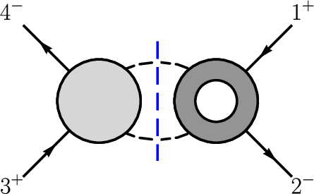
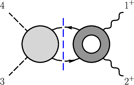
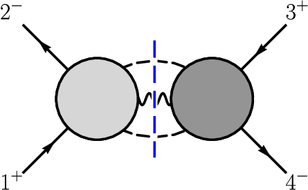
Figure 2: Unitarity cuts relevant for the extraction of anomalous dimensions from two-loop form factors, using the same notation as in Figure 1. The darker blobs indicate a higher-dimension operator insertion. The blobs with a hole indicate a one-loop form factor or amplitude.

Next consider two loops. Expanding Eq. (20) through this order, we obtain

[Δγ(1)i​j+δi​jβ(1)∂]Fj(1)+[Δγ(2)i​j+δi​jβ(2)∂]Fj(0)−iπ12[Δγ(1)i​k+δi​kβ(1)∂][Δγ(1)k​j+δk​jβ(1)∂]Fj(0)=−1π(ℳFi)(2).\displaystyle\begin{split}&\left[\Delta\gamma^{(1)}_{ij}+\delta_{ij}\beta^{(1)}\partial\right]F_{j}^{(1)}+\left[\Delta\gamma^{(2)}_{ij}+\delta_{ij}\beta^{(2)}\partial\right]F_{j}^{(0)}\\ &\hskip 42.67912pt\hbox{}-i\pi\,\frac{1}{2}\left[\Delta\gamma^{(1)}_{ik}+\delta_{ik}\beta^{(1)}\partial\right]\left[\Delta\gamma^{(1)}_{kj}+\delta_{kj}\beta^{(1)}\partial\right]F_{j}^{(0)}=-\frac{1}{\pi}(\mathcal{M}F_{i})^{(2)}\,.\end{split} (27)

On the right-hand side of this equation, (ℳ​Fi)(2)(\mathcal{M}F_{i})^{(2)} denotes collectively the three two-loop unitarity cuts displayed in Figure 2,

(ℳ​Fi)(2)\displaystyle(\mathcal{M}F_{i})^{(2)} =∑k=2n∑c[(ℳk→2c)(1)⊗Fn−k+2,i(0)+(ℳk→2c)(0)⊗Fn−k+2,i(1)\displaystyle=\sum_{k=2}^{n}\sum_{c}\,\left[(\mathcal{M}^{c}_{k\rightarrow 2})^{(1)}\otimes F_{n-k+2\,,i}^{(0)}+(\mathcal{M}^{c}_{k\rightarrow 2})^{(0)}\otimes F_{n-k+2\,,i}^{(1)}\right.
+(ℳk→3c)(0)⊗Fn−k+3,i(0)].\displaystyle\left.\hskip 85.35826pt+(\mathcal{M}^{c}_{k\rightarrow 3})^{(0)}\otimes F_{n-k+3\,,i}^{(0)}\right]. (28)

In the first term we find two-particle cuts composed of the one-loop amplitude and the tree-level higher-dimension form factor depicted in Figure 2(a). These are

(ℳk→21⋯k)(1)⊗Fn−k+2,i(0)=∫dLIPS2∑h1,h2⟨1⋯k|ℳ|ℓ1h1ℓ2h2⟩(1)⟨ℓ1h1ℓ2h2⋯n|𝒪i|0⟩(0)\displaystyle(\mathcal{M}^{1\cdots k}_{k\rightarrow 2})^{(1)}\otimes F_{n-k+2\,,i}^{(0)}=\int d\text{LIPS}_{2}\sum_{h_{1},h_{2}}\langle 1\cdots k|\mathcal{M}|\ell_{1}^{h_{1}}\ell_{2}^{h_{2}}\rangle^{(1)}\,\langle\ell_{1}^{h_{1}}\ell_{2}^{h_{2}}\cdots n|\mathcal{O}_{i}|0\rangle^{(0)}
=∫d​LIPS2​∑h1,h2A(1)​(1,⋯,k,−ℓ1−h1,−ℓ2−h2)​Fi(0)​(ℓ1h1,ℓ2h2,⋯,n).\displaystyle\hskip 56.9055pt=\int d\text{LIPS}_{2}\sum_{h_{1},h_{2}}A^{(1)}(1,\cdots,k,-\ell_{1}^{-h_{1}},-\ell_{2}^{-h_{2}})\,F_{i}^{(0)}(\ell_{1}^{h_{1}},\ell_{2}^{h_{2}},\cdots,n)\,. (29)

Similarly, the second term, shown in Figure 2(b), is a combination of cuts composed by the tree-level amplitude and the one-loop higher-dimension operator, which are

(ℳk→21⋯k)(0)⊗Fn−k+2,i(1)=∫dLIPS2∑h1,h2⟨1⋯k|ℳ|ℓ1h1ℓ2h2⟩(1)⟨ℓ1h1ℓ2h2⋯n|𝒪i|0⟩(0)\displaystyle(\mathcal{M}^{1\cdots k}_{k\rightarrow 2})^{(0)}\otimes F_{n-k+2\,,i}^{(1)}=\int d\text{LIPS}_{2}\sum_{h_{1},h_{2}}\langle 1\cdots k|\mathcal{M}|\ell_{1}^{h_{1}}\ell_{2}^{h_{2}}\rangle^{(1)}\,\langle\ell_{1}^{h_{1}}\ell_{2}^{h_{2}}\cdots n|\mathcal{O}_{i}|0\rangle^{(0)}
=∫d​LIPS2​∑h1,h2A(0)​(1,⋯,k,−ℓ1−h1,−ℓ2−h2)​Fi(1)​(ℓ1h1,ℓ2h2,⋯,n).\displaystyle\hskip 56.9055pt=\int d\text{LIPS}_{2}\sum_{h_{1},h_{2}}A^{(0)}(1,\cdots,k,-\ell_{1}^{-h_{1}},-\ell_{2}^{-h_{2}})\,F_{i}^{(1)}(\ell_{1}^{h_{1}},\ell_{2}^{h_{2}},\cdots,n)\,. (30)

Finally, the third term is composed of three-particle cuts involving two tree-level objects, as in Figure 2(c)

(ℳk→31⋯k)(0)⊗Fn−k+3,i(1)=∫dLIPS3∑h1,h2,h3⟨1⋯k|ℳ|ℓ1h1ℓ2h2ℓ3h3⟩(0)⟨ℓ1h1ℓ2h2ℓ3h3⋯n|𝒪i|0⟩(0)\displaystyle(\mathcal{M}^{1\cdots k}_{k\rightarrow 3})^{(0)}\otimes F_{n-k+3\,,i}^{(1)}=\int d\text{LIPS}_{3}\!\!\sum_{h_{1},h_{2},h_{3}}\!\!\langle 1\cdots k|\mathcal{M}|\ell_{1}^{h_{1}}\ell_{2}^{h_{2}}\ell_{3}^{h_{3}}\rangle^{(0)}\langle\ell_{1}^{h_{1}}\ell_{2}^{h_{2}}\ell_{3}^{h_{3}}\cdots n|\mathcal{O}_{i}|0\rangle^{(0)}
=∫d​LIPS3​∑h1,h2,h3A(0)​(1,⋯,k,−ℓ1−h1,−ℓ2−h2,−ℓ3−h3)​Fi(0)​(ℓ1h1,ℓ2h2,ℓ3h3,⋯,n).\displaystyle\hskip 0.0pt=\int d\text{LIPS}_{3}\!\!\sum_{h_{1},h_{2},h_{3}}\!\!A^{(0)}(1,\cdots,k,-\ell_{1}^{-h_{1}},-\ell_{2}^{-h_{2}},-\ell_{3}^{-h_{3}})F_{i}^{(0)}(\ell_{1}^{h_{1}},\ell_{2}^{h_{2}},\ell_{3}^{h_{3}},\cdots,n)\,. (31)

A parameterization analogous to (25) for the three-particle cut is given in Ref. Caron-Huot:2016cwu. We will not evaluate any three-particle cuts in the present work, so we refer the reader to this work for more details.

We can rearrange Eq. (27) to put it into a more convenient form for extracting two-loop anomalous dimensions. First, note that the imaginary part of Eq. (27)

−iπ12[Δγi​k(1)+δi​kβ(1)∂][Δγk​j(1)+δk​jβ(1)∂]Fj(0)\displaystyle-i\pi\,\frac{1}{2}\left[\Delta\gamma^{(1)}_{ik}+\delta_{ik}\beta^{(1)}\partial\right]\left[\Delta\gamma^{(1)}_{kj}+\delta_{kj}\beta^{(1)}\partial\right]F_{j}^{(0)} =−1π​Im​(ℳ​Fi)(2),\displaystyle=-\frac{1}{\pi}\text{Im}(\mathcal{M}F_{i})^{(2)}\,, (32)

does not feature the two-loop anomalous dimensions. Using the optical theorem again, we write its right-hand side in terms of unitarity cuts

Im​(ℳ​Fi)(2)=(ℳ​ℳ​Fi)(2),\text{Im}(\mathcal{M}F_{i})^{(2)}=(\mathcal{M}\mathcal{M}F_{i})^{(2)}\,, (33)

where the relevant cuts are the iterated two-particle cuts in Fig. 3. For instance (ℳ​ℳ​Fi)(2)(\mathcal{M}\mathcal{M}F_{i})^{(2)} contains terms of the form

∫dLIPS2dLIPS2′∑h1,h2∑h1′,h2′⟨⋯|ℓ1h1ℓ2h2⟩(0)⟨ℓ1h1ℓ2h2⋯|ℓ1′h1′ℓ2′h2′⟩(0)⟨ℓ1′h1′ℓ2′h2′⋯|𝒪i|0⟩(0),\displaystyle\!\!\int d\text{LIPS}_{2}d\text{LIPS}_{2}^{\prime}\sum_{h_{1},h_{2}}\sum_{h^{\prime}_{1},h^{\prime}_{2}}\langle\cdots|\ell_{1}^{h_{1}}\ell_{2}^{h_{2}}\rangle^{(0)}\langle\ell_{1}^{h_{1}}\ell_{2}^{h_{2}}\cdots|\ell_{1^{\prime}}^{h^{\prime}_{1}}\ell_{2^{\prime}}^{h^{\prime}_{2}}\rangle^{(0)}\langle\ell_{1^{\prime}}^{h^{\prime}_{1}}\ell_{2^{\prime}}^{h^{\prime}_{2}}\cdots|\mathcal{O}_{i}|0\rangle^{(0)}\,, (34)

which correspond to cuts of the type in Fig. 3(a). Note that Eq. (33) does not include a factor of 1/21/2 from the optical theorem because the imaginary part can arise from cutting either the one-loop amplitude or form factor, which give identical contributions.

Eq. (32) does not contain the two-loop anomalous dimensions but instead captures the exponentiation of one-loop anomalous dimensions and the associated logarithms. Nonetheless (33) can be used to simplify the real part of Eq. (27), which yields

[Δγi​j(1)+δi​jβ(1)∂]ReFj(1)+[Δγi​j(2)+δi​jβ(2)∂]Fj(0)\displaystyle\left[\Delta\gamma^{(1)}_{ij}+\delta_{ij}\beta^{(1)}\partial\right]\text{Re}F_{j}^{(1)}+\left[\Delta\gamma^{(2)}_{ij}+\delta_{ij}\beta^{(2)}\partial\right]F_{j}^{(0)} (35)
=−1π​Re​(ℳ​Fi)(2)=−1π​(ℳ​Fi−ℳ​ℳ​Fi)(2).\displaystyle\hskip 85.35826pt=-\frac{1}{\pi}\text{Re}(\mathcal{M}F_{i})^{(2)}=-\frac{1}{\pi}(\mathcal{M}F_{i}-\mathcal{M}\mathcal{M}F_{i})^{(2)}\,.

Note that the right-hand side can be rewritten using

(ℳ​Fi−ℳ​ℳ​Fi)(2)=[(ℳ−12​ℳ​ℳ)​(Fi−12​ℳ​Fi)](2)=[Re​(ℳ)​Re​(Fi)](2),\displaystyle(\mathcal{M}F_{i}-\mathcal{M}\mathcal{M}F_{i})^{(2)}=\left[\left(\mathcal{M}-\frac{1}{2}\mathcal{M}\mathcal{M}\right)\left(F_{i}-\frac{1}{2}\mathcal{M}F_{i}\right)\right]^{(2)}=\left[\text{Re}(\mathcal{M})\text{Re}(F_{i})\right]^{(2)}\,,\hskip 22.76228pt (36)

and with this we arrive at

[Δγi​j(1)+δi​jβ(1)∂]ReFj(1)+[Δγi​j(2)+δi​jβ(2)∂]Fj(0)=−1π[Re(ℳ)Re(Fi)](2).\displaystyle\left[\Delta\gamma^{(1)}_{ij}+\delta_{ij}\beta^{(1)}\partial\right]\text{Re}F_{j}^{(1)}+\left[\Delta\gamma^{(2)}_{ij}+\delta_{ij}\beta^{(2)}\partial\right]F_{j}^{(0)}=-\frac{1}{\pi}\left[\text{Re}(\mathcal{M})\text{Re}(F_{i})\right]^{(2)}\,. (37)

We use this equation to extract two-loop anomalous dimensions. In practice Eq. (37) simply instructs us to drop the imaginary parts of the one-loop matrix elements when calculating the cuts in Figs. 2(a) and 2(b). On the left-hand side, we now see the appearance of one-loop anomalous dimensions and the β\beta-function, as well as the one-loop form factor Fi(1)F_{i}^{(1)}. The two-loop UV anomalous dimension γi​jUV⁡(2)\gamma_{ij}^{\rm UV(2)} contained in Δ​γi​j(2)\Delta\gamma^{(2)}_{ij} is the object of interest, but to extract it we first need to remove γi​jIR⁡(2)\gamma_{ij}^{\rm IR(2)}, which requires an understanding of the IR singularities, which we discuss below.

Refer to caption

(a)

Refer to caption

(b)

Figure 3: Iterated two-particle cuts that appear on the right-hand side of Eq. (33).

2.3.1 Simplifying strategies

A strategy that greatly simplifies the analysis is to choose an external state with the minimal number of external legs that is sensitive to the operator of interest, i.e. select the operator’s minimal form factor. In this way we can avoid terms of the form β(n)​∂Fi(0)\beta^{(n)}\partial F^{(0)}_{i} in Eqs. (27) and (37), since, under this choice, Fi(0)F^{(0)}_{i} is local, and thus does not depend on the dimension-four couplings, g(4)g^{(4)}. This strategy was used in Ref. NonrenormLength to prove nonrenormalization theorems at the first loop order where diagrams exist.

More generally, the β\beta-function can no longer be eliminated by using minimal form factors whenever the one-loop form factor with an 𝒪i\mathcal{O}_{i} insertion, Fi(1)F^{(1)}_{i}, produces a nonzero result with the chosen external states. In addition, the β\beta-function acting on the one-loop anomalous-dimension matrix is nonzero if the matrix elements themselves are nonzero. For example, to determine the renormalization of 𝒪F3\mathcal{O}_{F^{3}} by itself at two loops, we would evaluate Eq. (37) with the external state ⟨1+​2+​3+|\langle 1^{+}2^{+}3^{+}|. In this case the term β(2)​∂FF3(0)\beta^{(2)}\partial F_{F^{3}}^{(0)} would vanish, though the term β(1)​∂FF3(1)\beta^{(1)}\partial F_{F^{3}}^{(1)} would remain.

Unlike the β\beta-function, the IR anomalous dimensions are non-trivial to eliminate. Ref. Caron-Huot:2016cwu removes them by subtracting, at the integrand level, form factors of global symmetry currents, such as the stress-tensor, which are UV finite but contain the same IR divergences. Alternatively, one can use the same on-shell methods to calculate them and subtract them after integration. At one loop, the structure of infrared divergences is well understood IRBasicPapers; IRLaterPapers; StermanBook, and it is straightforward to subtract them after integration. We explain how to carry this out at the level of the amplitudes in the next section. Furthermore, whenever we are interested in a leading off-diagonal element of the anomalous dimension matrix, the IR anomalous dimensions does not appear, since the infrared divergences are diagonal in the operators (excluding color).

Finally, form factors are useful for operators with only two or three external fields, since they allow nonzero results when kinematics would otherwise set amplitudes with fewer than four external particles to zero. Here we generally set the operator momentum insertion q=0q=0 and work in terms of amplitudes whenever possible, i.e. whenever there are four or more external states.

2.4 Comments on evanescent operators

When extracting anomalous dimensions from UV divergences in dimensional regularization one must carefully keep track of evanescent operators Evanescent; EvanescentFinite. These operators are non-trivial in DD-dimensions, but whose matrix elements vanish for any choice of external four-dimensional states. In the context of the SMEFT an example of an evanescent operator would be the Lorentz–Fierz identities

𝒪Fierz,L\displaystyle\mathcal{O}_{\rm Fierz,L} =(ψ¯​γμLm​ψLn)​(ψ¯​γμLp​ψLr)+(ψ¯​γμLp​ψLn)​(ψ¯​γμLm​ψLr),\displaystyle=(\overline{\psi}{}^{m}_{L}\gamma^{\mu}\psi^{n}_{L})(\overline{\psi}{}^{p}_{L}\gamma_{\mu}\psi^{r}_{L})+(\overline{\psi}{}^{p}_{L}\gamma^{\mu}\psi^{n}_{L})(\overline{\psi}{}^{m}_{L}\gamma_{\mu}\psi^{r}_{L})\,,
𝒪Fierz,R\displaystyle\mathcal{O}_{\rm Fierz,R} =(ψ¯​γμRm​ψRn)​(ψ¯​γμRp​ψRr)+(ψ¯​γμRp​ψRn)​(ψ¯​γμRm​ψRr),\displaystyle=(\overline{\psi}{}^{m}_{R}\gamma^{\mu}\psi^{n}_{R})(\overline{\psi}{}^{p}_{R}\gamma_{\mu}\psi^{r}_{R})+(\overline{\psi}{}^{p}_{R}\gamma^{\mu}\psi^{n}_{R})(\overline{\psi}{}^{m}_{R}\gamma_{\mu}\psi^{r}_{R})\,, (38)

(where we raised the flavor indices for convenience) which are identically zero in four but not in arbitrary dimensions. More generally one can easily construct such operators by antisymmetrizing over five or more Lorentz indices. In the context of our model, an example of such an evanescent operator is

(ψ¯γ[αγμγνγσγρ]ψ)(ψ¯γ[αγμγνγσγρ]ψ).(\overline{\psi}\gamma_{[\alpha}\gamma_{\mu}\gamma_{\nu}\gamma_{\sigma}\gamma_{\rho]}\psi)(\overline{\psi}\gamma^{[\alpha}\gamma^{\mu}\gamma^{\nu}\gamma^{\sigma}\gamma^{\rho]}\psi)\,. (39)

One-loop diagrams might contain a 1/ϵ1/\epsilon divergence proportional to the matrix element of an evanescent operator. While this does not affect one-loop anomalous dimensions because we can take the external states to be four-dimensional, when inserted in a higher-loop diagram in the context of dimensional regularization such evanescent operators are activated and can generate both UV divergent and finite contributions. In fact, they are needed to properly subtract subdivergences. These effects must be taken into account in order to correctly extract two-loop UV divergences and their associated anomalous dimension. In practice we can deal with the effects of evanescent operators Evanescent; EvanescentFinite, but the number of them grows with dimension and loop order (especially in the presence of fermions). For this reason it would be desirable to avoid them when possible, since they are a technical complication due to the use of dimensional regularization, and ultimately we would expect that they do not affect the physics TwoLoopGravitySimplified1.

We expect the on-shell methods presented above to completely sidestep the issue of evanescent operators when obtaining anomalous dimension, at least through two loops. Ref. TwoLoopGravitySimplified2 provides a nontrivial demonstration that complications from evanescent operators can be completely sidestepped using on-shell methods and by focusing on renormalization-scale dependence instead of divergences. In the two-loop formulas used here, anomalous dimensions and associated logarithms are given directly in terms of four-dimensional unitarity cuts of tree and one-loop objects. This automatically eliminates most of the evanescent dependence, except for finite shifts in one-loop matrix elements with evanescent operator insertions. We expect that any remaining evanescent dependence in the one-loop amplitudes or form factors to be eliminated by finite renormalizations EvanescentFinite. Given the usual subtleties of dealing with evanescent operators, it would, of course, be important to explicitly verify that including or not including evanescent operators in the one- and two-loop anomalous dimension matrix amounts to a scheme choice.

2.5 Anomalous dimensions and non-interference

As noted in Ref. NonInterference helicity selection rules imply the non-interference of SMEFT tree-level matrix elements when constructing cross sections. This has important consequences in the context of the SMEFT, where the possibility of measuring the coefficient of higher-dimension operators at colliders can be impacted by the vanishings in the interference of the Standard-Model tree amplitudes and those of higher-dimension operators, when computing cross sections. A connection between one-loop anomalous dimension and interference terms can be seen in Eq. (22), where, upon setting q=0q=0, the form factors become amplitudes and the right-hand side directly captures the interference of tree-level dimension-four and dimension-six amplitudes. Note that this holds even when the anomalous dimension is not zero, in which case this equation relates the interference terms to simpler objects, namely the one-loop anomalous dimensions and tree-level matrix elements. Of course, in a realistic cross-section calculation one would not integrate over the full phase space, due to experimental cuts.

At two loops the connection between zeros in the anomalous dimensions and non-interference is not as direct, since it requires cancellations between both sides of Eq. (27). Eq. (32) shows that, in general, the imaginary part of the interference term is given by the square of one-loop anomalous dimensions times tree-level matrix elements. Instead of non-interference, Eq. (35) shows that a vanishing two-loop anomalous dimension would imply that the real part of interference term is simply is related to the product of one-loop anomalous dimensions and one-loop matrix elements. It would be interesting to further investigate the consequences stemming from these observations, even in the presence of experimental cuts.

3 One-loop amplitudes and anomalous dimensions

In this section we describe our generalized unitarity calculation of the one-loop amplitudes with an insertion of a higher-dimensional operator in our simplified model. We then extract the one-loop anomalous dimension matrix of this theory. Finally, we comment on the structure of rational terms in the amplitudes and on the ability to set some of them to zero with a judicious scheme choice. The results in this section are building blocks needed for the two-loop analysis in the next section. In addition, they provide one-loop anomalous dimensions that can be cross-checked against those in Refs. Manohar123.

3.1 One-loop amplitudes from generalized unitarity

The generalized unitarity method GeneralizedUnitarity1; ChiralOnShell; GeneralizedUnitarity2 for constructing one-loop amplitudes can be found in various reviews, for example see Ref. UnitarityReviews, but here we briefly review the procedure for the one-loop case. To construct the full one-loop amplitudes to all orders in the dimensional-regularization parameter ϵ\epsilon, we begin with the DD-dimensional four-point tree-level amplitudes with or without insertions of the dimension-6 operators (given in Appendix B). By using DD-dimensional tree amplitudes, we ensure that the cuts appropriately capture the coefficients of the DD-dimensional box, triangle, and bubble scalar integrals that form a basis for the full one-loop amplitudes, as in Eq. (13). In general, the coefficients have ϵ\epsilon dependence, and expanding in ϵ\epsilon produces rational terms that would not automatically be included if a purely four-dimensional approach to the cuts were used GeneralizedUnitarity1. Besides ϵ\epsilon, the coefficients only depend on the Mandelstam invariants s=(k1+k2)2s=(k_{1}+k_{2})^{2}, t=(k2+k3)2t=(k_{2}+k_{3})^{2} and u=(k1+k3)2u=(k_{1}+k_{3})^{2}.

We construct the cuts in the standard way. For example, the integrand-level ss-channel cut with an 𝒪n\mathcal{O}_{n} operator insertion is given by

∑i𝒞[i]([as​t4,n⁡[i]I4,s​t+as​u4,n⁡[i]I4,s​u+as3,n⁡[i]I3,s+as2,n⁡[i]I2,s]|ℓ2=0)=∑states ∑j𝒞[j]​An(0)​(1,2,ℓ1h1,ℓ2h2)[j]​∑k𝒞[k]​A(0)​(−ℓ2h2,−ℓ1h1,3,4)[k]+∑states ∑j𝒞[j]A(0)(1,2,ℓh11,ℓh22)[j]∑k𝒞[k]An(0)(−ℓh22,−ℓh11,3,4)[k],\displaystyle\begin{split}\sum_{i}&\mathcal{C}^{[i]}\left(\left[a^{st}_{4,n[i]}I_{4,st}+a^{su}_{4,n[i]}I_{4,su}+a^{s}_{3,n[i]}I_{3,s}+a^{s}_{2,n[i]}I_{2,s}\right]\Big\rvert_{\ell^{2}=0}\,\right)\\ &=\sum_{\text{states }}\sum_{j}\mathcal{C}^{[j]}A_{n}^{(0)}(1,2,\ell^{h_{1}}_{1},\ell^{h_{2}}_{2})_{[j]}\sum_{k}\mathcal{C}^{[k]}A^{(0)}(-\ell^{h_{2}}_{2},-\ell^{h_{1}}_{1},3,4)_{[k]}\\ &\quad+\sum_{\text{states }}\sum_{j}\mathcal{C}^{[j]}A^{(0)}(1,2,\ell^{h_{1}}_{1},\ell^{h_{2}}_{2})_{[j]}\sum_{k}\mathcal{C}^{[k]}A_{n}^{(0)}(-\ell^{h_{2}}_{2},-\ell^{h_{1}}_{1},3,4)_{[k]}\,,\end{split} (40)

where the sum over states includes the helicity and the color, and, for this case, ℓ2=−(ℓ1+k1+k2)\ell_{2}=-(\ell_{1}+k_{1}+k_{2}). The 𝒞[i]\mathcal{C}^{[i]} are the appropriate color factors for the associated amplitudes. Since the cut legs are on-shell, where ℓ12=ℓ22=0\ell_{1}^{2}=\ell_{2}^{2}=0. Often, the external particles will restrict An(0)A_{n}^{(0)} to be nonzero only for certain cuts or placements within the cuts, depending on the field content of the operator inserted.

(a)
Refer to caption

(b)
Refer to caption

(c)
Refer to caption

Refer to caption

(d)

Refer to caption

(e)

Figure 4: The necessary cut for constructing a two-fermion, two-vector amplitude. For an amplitude with an insertion of a higher-dimension operator, one should insert the operator into either side of the diagrams when possible. The wavy lines are vector bosons, the lines with arrows fermions and the dashed lines scalars.

As an example, the cuts of the amplitude AF3(1)​(1ψ​2ψ¯​3 4)A^{(1)}_{{F^{3}}}(1_{\vphantom{\overline{\psi}}\psi}2_{\overline{\psi}}3\,4), are shown in Figure 4, where the operator 𝒪F3\mathcal{O}_{{F^{3}}} should be inserted on either side of the cuts, when the tree amplitudes exist. Other amplitudes with four-point operators require only the cuts corresponding to their correct external particles. The color factors 𝒞[j]​𝒞[k]\mathcal{C}^{[j]}\mathcal{C}^{[k]} can be reduced to the appropriate color basis of the full amplitude, 𝒞[i]\mathcal{C}^{[i]}, based on the external particles. Doing so determines the contribution from each color-decomposed cut.

We evaluate the cuts using the DD-dimensional state sum completeness relations,

ϵi∗μ⊙ϵiν=∑states ​hϵi∗(h)​μ​ϵi(h)​ν=−gμ​ν+qμ​kiν+kiμ​qνq⋅ki,u¯i⊙ui=∑states ​hu¯i(h)​ui(h)=k̸i,\displaystyle\begin{split}\epsilon_{i}^{*\mu}\odot\epsilon_{i}^{\nu}=\sum_{\text{states }h}\epsilon_{i}^{*(h)\mu}\epsilon_{i}^{(h)\nu}&=-g^{\mu\nu}+\frac{q^{\mu}k_{i}^{\nu}+k_{i}^{\mu}q^{\nu}}{q\cdot k_{i}}\,,\\[5.0pt] \overline{u}_{i}\odot u_{i}=\sum_{\text{states }h}&\overline{u}^{(h)}_{i}u^{(h)}_{i}=\not{k}_{i}\,,\end{split} (41)

where qq is an arbitrary reference vector with q2=0q^{2}=0.

The next task is to merge the cuts and to integrate. One can merge the cuts at the level of the integrand to find a single integrand that has the correct cuts in all channels. However, is it is generally simpler to merge the integrated results from each cut, treating each cut as an off-shell object, but dropping contributions that do not have a cut in the given channel. Integration is done by projecting each cut for a given process onto a basis of gauge-invariant tensors, as described in more detail in Appendix A. Although the methods we use to extract anomalous dimensions do not require us to keep track of evanescent divergences, because the projection technique is fully DD dimensional, we track them and confirm that they do not enter our calculations of various entries in the two-loop anomalous-dimension matrix. An alternative is to use spinor-helicity methods SpinorHelicity which are much more powerful when the number of external legs increases. These have been successfully used for both chiral ChiralOnShell and higher-loop calculations TwoLoopHelicityExample, but then additional care is needed to deal with subtleties that arise from using dimensional regularization.

After projection, the cut integrand is rewritten in terms of inverse propagators. We reduce the remaining integrals to the basis of scalar integrals in Eq. (13) using integration by parts relations as implemented in FIRE FIRE. Cut merging is then straightforward, as the coefficients of integrals in the merged amplitude can be read directly off the results from each cut, summed over the possible particles crossing the cut. For example, the ss-channel cut in Eq. (40) yields the coefficients of the ss-channel bubble and triangle, as well as those of the (s,t)(s,t) and (s,u)(s,u) boxes in Eq. (13).

The full set of DD-dimensional four-point one-loop amplitudes for the dimension-six operators in our model are given in the ancillary file AttachedFiles. These expressions are valid to all orders in ϵ\epsilon, but to obtain the finite, renormalized expressions needed to feed into our calculation of two-loop anomalous dimensions, we need to subtract the UV poles.

The one-loop amplitudes are IR divergent. The IR singularities of gauge theories are well understood IRBasicPapers; IRLaterPapers; IRModernPapers; StermanBook, and can be expressed in terms of lower-loop amplitudes involving the same operator insertion and external particles. The explicit form of the one-loop infrared singularity, for example, is given by

Ai(1)=\displaystyle A_{i}^{(1)}=\hbox{} 𝑰(1)​Ai(0),\displaystyle\boldsymbol{I}^{(1)}A_{i}^{(0)}\,, (42)

where the IR operator 𝑰(1)\boldsymbol{I}^{(1)} is given by IRBasicPapers; IRLaterPapers; IRModernPapers55 5 The difference with the formulas in those references is due to our normalization of the S​U​(N)SU(N) generators.

𝑰(1)\displaystyle\boldsymbol{I}^{(1)} =eϵ​γEΓ⁡(1−ϵ)​∑p=1n∑q≠p𝑻p⋅𝑻q2​[γcuspIR⁡(1)ϵ2−γc,pIR⁡(1)𝑻p2​1ϵ]​(−μ22​kp⋅kq)ϵ,\displaystyle=\frac{e^{\epsilon\gamma_{E}}}{\Gamma(1-\epsilon)}\sum_{p=1}^{n}\sum_{q\neq p}\frac{\boldsymbol{T}_{p}\cdot\boldsymbol{T}_{q}}{2}\left[\frac{\gamma^{\rm IR\,(1)}_{\rm cusp}}{\epsilon^{2}}-\frac{\gamma^{\rm IR\,(1)}_{{\rm c},\,p}}{\boldsymbol{T}_{p}^{2}}\frac{1}{\epsilon}\right]\left(\frac{-\mu^{2}}{2k_{p}{\cdot}k_{q}}\right)^{\epsilon}\,, (43)

where the sums are over external particles. The color charge 𝑻p={Tpa}\boldsymbol{T}_{p}=\{T^{a}_{p}\} is a vector with respect to the generator label aa and a SU(NN) matrix with respect to the outgoing particle pp. The infrared divergence includes a 1/ϵ21/\epsilon^{2} pole, with coefficient given by the cusp anomalous dimension γcuspIR⁡(1)=4​g~2\gamma^{\rm IR\,(1)}_{\rm cusp}=4\widetilde{g}^{2}, and 1/ϵ1/\epsilon poles, with coefficient given by the collinear anomalous dimension of particle pp given in Eq. (16). By obtaining the IR dependence of the one-loop amplitudes from Eq. (42), we can subtract it from the full one-loop amplitudes. As always, the definition of the IR-divergent parts carries with it some arbitrariness as to which finite pieces are included.66 6 In physical quantities this arbitrariness cancels between real emission and virtual contributions.

The remaining poles in ϵ\epsilon are UV poles, which we then match to the appropriate tree-level counterterm amplitude containing an insertion of the operator 𝒪j\mathcal{O}_{j}. A complication is that there can be multiple operators corresponding to the same external particle content, but with different color structures. Therefore, in these cases the coefficient of a single color factor in the loop amplitude is insufficient for the purpose of determining the anomalous dimensions, and in principle all the color factors for the given process and operator insertion must be considered simultaneously. For example, the one-loop amplitude with an insertion of the 𝒪(D​φ2​ψ2)2\mathcal{O}_{(D\varphi^{2}\psi^{2})_{2}} operator and four external scalars determines the renormalization of both the 𝒪(D2​φ4)1\mathcal{O}_{(D^{2}\varphi^{4})_{1}} and the 𝒪(D2​φ4)2\mathcal{O}_{(D^{2}\varphi^{4})_{2}} operators, where the operators are given in Table 1.

In some cases the IR structure is trivial, e.g. when the IR anomalous dimensions are zero simply because there are no lower-loop amplitudes for a given operator and given external state. Our examples in Section 4 follow this pattern. For instance, in the example of 𝒪(D2​φ4)1\mathcal{O}_{(D^{2}\varphi^{4})_{1}} renormalizing 𝒪(ψ4)1\mathcal{O}_{(\psi^{4})_{1}} at two loops, there is no tree level or one-loop amplitude with an insertion of 𝒪(D2​φ4)1\mathcal{O}_{(D^{2}\varphi^{4})_{1}} which has an external state of four fermions, simply due to the lack of Feynman diagrams. Since the full IR dependence is proportional to lower-loop amplitudes, this implies there cannot be an IR divergence at two loops. This same reasoning underpinned the non-renormalization theorem in Ref. NonrenormLength. More generally, one needs to account for the infrared singularities.

3.2 One-loop UV anomalous dimensions

After subtracting the IR singularities, the only remaining 1/ϵ1/\epsilon poles in the amplitudes correspond to the desired one-loop anomalous dimensions,

c˙F3=\displaystyle\dot{c}_{{F^{3}}}=\hbox{} g~2​(12​N−3​b0)​cF3,\displaystyle\widetilde{g}^{2}(12N-3b_{0})c_{{F^{3}}}\,,
c˙(φ2​F2)1=\displaystyle\dot{c}_{{(\varphi^{2}F^{2})_{1}}}=\hbox{} g~2​(−5​cF3−(3​N2−7)+2​N​b0N​c(φ2​F2)1+N2−4N2​c(φ2​F2)2)\displaystyle\widetilde{g}^{2}\biggl(-5c_{F_{3}}-\frac{(3N^{2}-7)+2Nb_{0}}{N}c_{{(\varphi^{2}F^{2})_{1}}}+\frac{N^{2}-4}{N^{2}}c_{{(\varphi^{2}F^{2})_{2}}}\biggr)
+λ~​ 4​(1+N)​c(φ2​F2)1,\displaystyle+\widetilde{\lambda}\,4(1+N)c_{{(\varphi^{2}F^{2})_{1}}}\,,
c˙(φ2​F2)2=\displaystyle\dot{c}_{{(\varphi^{2}F^{2})_{2}}}=\hbox{} g~2​(−N​cF3+2​c(φ2​F2)1+2​N2−5−2​N​b0N​c(φ2​F2)2)+λ~​ 4​c(φ2​F2)2,\displaystyle\widetilde{g}^{2}\left(-Nc_{{F^{3}}}+2c_{{(\varphi^{2}F^{2})_{1}}}+\frac{2N^{2}-5-2Nb_{0}}{N}c_{{(\varphi^{2}F^{2})_{2}}}\right)+\widetilde{\lambda}\,4c_{{(\varphi^{2}F^{2})_{2}}},
c˙(D2​φ4)1=\displaystyle\dot{c}_{{(D^{2}\varphi^{4})_{1}}}=\hbox{} g~2​(3​(N+1)N​c(D2​φ4)1+2​(N−2)​(Ns+9)3​N​c(D2​φ4)2+43​N−2N​c(D​φ2​ψ2)2w​w)\displaystyle\widetilde{g}^{2}\left(\frac{3(N+1)}{N}c_{{(D^{2}\varphi^{4})_{1}}}+\frac{2(N-2)(N_{s}+9)}{3N}c_{{(D^{2}\varphi^{4})_{2}}}+\frac{4}{3}\frac{N-2}{N}c_{{(D\varphi^{2}\psi^{2})_{2}}}^{ww}\right)
+λ​ 12​c(D2​φ4)1,\displaystyle+\lambda\,12c_{{(D^{2}\varphi^{4})_{1}}}\,,
c˙(D2​φ4)2=\displaystyle\dot{c}_{{(D^{2}\varphi^{4})_{2}}}=\hbox{} g~2​(36​N​CF−(2​N−1)​(Ns+9)3​N​c(D2​φ4)2+3​(N−2)​(N+1)2​N​c(D2​φ4)1CLOSE\displaystyle\widetilde{g}^{2}\left(\frac{36NC_{F}-(2N-1)(N_{s}+9)}{3N}c_{{(D^{2}\varphi^{4})_{2}}}+\frac{3(N-2)(N+1)}{2N}c_{{(D^{2}\varphi^{4})_{1}}}\right.
OPEN+2​(2​N−1)3​N​c(D​φ2​ψ2)2w​w)+λ~​(2​(N−2)​c(D2​φ4)1+8​(N+1)​c(D2​φ4)2),\displaystyle\left.\hskip 14.22636pt\hbox{}+\frac{2(2N-1)}{3N}c_{{(D\varphi^{2}\psi^{2})_{2}}}^{ww}\right)+\widetilde{\lambda}\,\left(2(N-2)c_{{(D^{2}\varphi^{4})_{1}}}+8(N+1)c_{{(D^{2}\varphi^{4})_{2}}}\right),
c˙(D​φ2​ψ2)1p​r=\displaystyle\dot{c}_{{(D\varphi^{2}\psi^{2})_{1}}}^{pr}=\hbox{} 0,\displaystyle 0\,,
c˙(D​φ2​ψ2)2p​r=\displaystyle\dot{c}_{{(D\varphi^{2}\psi^{2})_{2}}}^{pr}=\hbox{} g~2​(13​Ns​c(D2​φ4)2​δp​r+13​(−9​N+Ns)​c(D​φ2​ψ2)2p​r+43​Nf​c(D​φ2​ψ2)2w​w​δp​rCLOSE\displaystyle\,\widetilde{g}^{2}\left(\frac{1}{3}N_{s}c_{{(D^{2}\varphi^{4})_{2}}}\delta_{pr}+\frac{1}{3}(-9N+N_{s})c_{{(D\varphi^{2}\psi^{2})_{2}}}^{pr}+\frac{4}{3}N_{f}c_{{(D\varphi^{2}\psi^{2})_{2}}}^{ww}\delta_{pr}\right.
OPEN−23​Nf​c(ψ4)1p​w​w​r−23​Nf​(2​c(ψ4)2p​r​w​w−1N​c(ψ4)2p​w​w​r)),\displaystyle\left.\hbox{}-\frac{2}{3}N_{f}c_{{(\psi^{4})_{1}}}^{pwwr}-\frac{2}{3}N_{f}\left(2c_{{(\psi^{4})_{2}}}^{prww}-\frac{1}{N}c_{{(\psi^{4})_{2}}}^{pwwr}\right)\right),
c˙(ψ4)1m​n​p​r=\displaystyle\dot{c}_{{(\psi^{4})_{1}}}^{mnpr}=\hbox{} g~2​6​(N2−1)N2​c(ψ4)2m​n​p​r,\displaystyle\widetilde{g}^{2}\frac{6\left(N^{2}-1\right)}{N^{2}}c_{{(\psi^{4})_{2}}}^{mnpr}\,,
c˙(ψ4)2m​n​p​r=\displaystyle\dot{c}_{{(\psi^{4})_{2}}}^{mnpr}=\hbox{} g~2​(−Ns3​(c(D​φ2​ψ2)2m​n​δp​r+c(D​φ2​ψ2)2p​r​δm​n)CLOSE\displaystyle\widetilde{g}^{2}\left(-\frac{N_{s}}{3}(c_{{(D\varphi^{2}\psi^{2})_{2}}}^{mn}\delta_{pr}+c_{{(D\varphi^{2}\psi^{2})_{2}}}^{pr}\delta_{mn})\right.
+23​Nf​(δm​n​c(ψ4)1p​w​w​r+δp​r​c(ψ4)1m​w​w​n)+6​c(ψ4)1m​n​p​r−3N​c(ψ4)2m​n​p​r\displaystyle\left.+\frac{2}{3}N_{f}(\delta_{mn}c_{{(\psi^{4})_{1}}}^{pwwr}+\delta_{pr}c_{{(\psi^{4})_{1}}}^{mwwn})+6c_{{(\psi^{4})_{1}}}^{mnpr}-\frac{3}{N}c_{{(\psi^{4})_{2}}}^{mnpr}\right.
OPEN+2​Nf3​N​(2​N​(δp​r​c(ψ4)2m​n​w​w+δm​n​c(ψ4)2p​r​w​w)−(δp​r​c(ψ4)2m​w​w​n+δm​n​c(ψ4)2p​w​w​r))).\displaystyle\left.+\frac{2N_{f}}{3N}(2N(\delta_{pr}c_{{(\psi^{4})_{2}}}^{mnww}+\delta_{mn}c_{{(\psi^{4})_{2}}}^{prww})-(\delta_{pr}c_{{(\psi^{4})_{2}}}^{mwwn}+\delta_{mn}c_{{(\psi^{4})_{2}}}^{pwwr}))\right)\,. (44)

Here NsN_{s} is left as a parameter to track contributions from scalar loops. In our model it should be set to unity. These anomalous dimensions have been extracted directly from the scattering amplitudes, and, as a cross-check, we also used the unitarity cut method explained in the previous section Caron-Huot:2016cwu for computing directly the anomalous dimensions. The structure of the anomalous dimension matrix is summarized in Table 2. It is worth pointing out the simplicity in the renormalization and mixing of (D​φ2​ψ2)1{(D\varphi^{2}\psi^{2})_{1}} and (ψ4)1{(\psi^{4})_{1}}, which is due to these operators being a product of global symmetry currents, which heavily constrains the kind of states they can overlap with. This is special in our model, which does not contain an Abelian gauge field. In the presence of the latter, the operators would be a product of gauge symmetry currents (just like (D​φ2​ψ2)2{(D\varphi^{2}\psi^{2})_{2}} and (ψ4)2{(\psi^{4})_{2}}) which are renormalized Collins:2005nj, so the anomalous dimension matrix will receive contributions proportional to the Abelian gauge coupling.

We use these results to verify a representative set of the one-loop anomalous dimension calculated in Ref. Manohar123, including entries from nearly all classes of operators. Additional details about this verification is given in Section 5. This provides a nontrivial check on our one-loop results, which we then feed into the two-loop anomalous dimension calculations.

F3{F^{3}} (φ2​F2)1{(\varphi^{2}F^{2})_{1}} (φ2​F2)2{(\varphi^{2}F^{2})_{2}} (D2​φ4)1{{(D^{2}\varphi^{4})_{1}}} (D2​φ4)2{{(D^{2}\varphi^{4})_{2}}} (D​φ2​ψ2)1{{(D\varphi^{2}\psi^{2})_{1}}} (D​φ2​ψ2)2{{(D\varphi^{2}\psi^{2})_{2}}} (ψ4)1{{(\psi^{4})_{1}}} (ψ4)2{{(\psi^{4})_{2}}}
F3{{F^{3}}} 0 0 0̸\not{0} 0̸\not{0} 0̸\not{0} 0̸\not{0} 0̸\not{0} 0̸\not{0}
(φ2​F2)1{{(\varphi^{2}F^{2})_{1}}} 0 0 0 0 0̸\not{0} 0̸\not{0}
(φ2​F2)2{{(\varphi^{2}F^{2})_{2}}} 0 0 0 0 0̸\not{0} 0̸\not{0}
(D2​φ4)1{{(D^{2}\varphi^{4})_{1}}} 0 0 0 0 0̸\not{0} 0̸\not{0}
(D2​φ4)2{{(D^{2}\varphi^{4})_{2}}} 0 0 0 0 0̸\not{0} 0̸\not{0}
(D​φ2​ψ2)1{{(D\varphi^{2}\psi^{2})_{1}}} 0 0 0 0 0 0 0 0 0
(D​φ2​ψ2)2{{(D\varphi^{2}\psi^{2})_{2}}} 0 0 0 0 0
(ψ4)1{{(\psi^{4})_{1}}} 0 0̸\not{0} 0̸\not{0} 0̸\not{0} 0̸\not{0} 0 0 0
(ψ4)2{{(\psi^{4})_{2}}} 0 0̸\not{0} 0̸\not{0} 0̸\not{0} 0̸\not{0} 0
Table 2: Structure of the zeros in the one-loop anomalous dimension matrix. The 0̸\not{0} entries indicate there are no contributing one-loop diagrams, whereas a 00 alone indicates that there are one-loop diagrams that could contribute, but actually give a vanishing result. The operators labeling the rows are renormalized by the operators labeling the columns.

3.3 Structure of one-loop amplitudes and rational terms

V+​V+​V+​V+V^{+}V^{+}V^{+}V^{+}

V+​V+​V+​V−V^{+}V^{+}V^{+}V^{-}

V+​V+​V−​V−V^{+}V^{+}V^{-}V^{-}

φ​φ​V+​V+\varphi\,\varphi\,V^{+}V^{+}

φ​φ​V+​V−\varphi\,\varphi\,V^{+}V^{-}

φ​φ​φ​φ\varphi\,\varphi\,\varphi\,\varphi

ψ−​ψ+​V+​V+\psi^{-}\psi^{+}V^{+}V^{+}

ψ−​ψ+​V+​V−\psi^{-}\psi^{+}V^{+}V^{-}

ψ−​ψ+​V−​V+\psi^{-}\psi^{+}V^{-}V^{+}

ψ+​ψ−​V−​V−\psi^{+}\psi^{-}V^{-}V^{-}

ψ+​ψ−​φ​φ\psi^{+}\psi^{-}\varphi\,\varphi

ψ+​ψ−​ψ+​ψ−\psi^{+}\psi^{-}\psi^{+}\psi^{-}

ψ+​ψ−​ψ−​ψ+\psi^{+}\psi^{-}\psi^{-}\psi^{+}

ψ+​ψ+​ψ−​ψ−\psi^{+}\psi^{+}\psi^{-}\psi^{-}

F3{{F^{3}}} L L R L R 0 L R R L 0 0 0 0
(φ2​F2)1{{(\varphi^{2}F^{2})_{1}}} R 0 R L R 0 0 0 0 0 0 0̸\not{0} 0̸\not{0} 0̸\not{0}
(φ2​F2)2{{(\varphi^{2}F^{2})_{2}}} R 0 R L L 0 0 0 0 0 0 0̸\not{0} 0̸\not{0} 0̸\not{0}
(D2​φ4)1{{(D^{2}\varphi^{4})_{1}}} 0̸\not{0} 0̸\not{0} 0̸\not{0} 0 0 L0 0̸\not{0} 0̸\not{0} 0̸\not{0} 0̸\not{0} 0 0̸\not{0} 0̸\not{0} 0̸\not{0}
(D2​φ4)2{{(D^{2}\varphi^{4})_{2}}} 0̸\not{0} 0̸\not{0} 0̸\not{0} R 0 L0 0̸\not{0} 0̸\not{0} 0̸\not{0} 0̸\not{0} L0 0̸\not{0} 0̸\not{0} 0̸\not{0}
(D​φ2​ψ2)1{{(D\varphi^{2}\psi^{2})_{1}}} 0̸\not{0} 0̸\not{0} 0̸\not{0} 0 0 0 0 0 0 0 L0 0 0 0
(D​φ2​ψ2)2{{(D\varphi^{2}\psi^{2})_{2}}} 0̸\not{0} 0̸\not{0} 0̸\not{0} R 0 L0 R 0 0 R L0 L0 L0 L0
(ψ4)1{{(\psi^{4})_{1}}} 0̸\not{0} 0̸\not{0} 0̸\not{0} 0̸\not{0} 0̸\not{0} 0̸\not{0} R 0 0 R L0 L L L
(ψ4)2{{(\psi^{4})_{2}}} 0̸\not{0} 0̸\not{0} 0̸\not{0} 0̸\not{0} 0̸\not{0} 0̸\not{0} R 0 0 R L0 L L L
R: rational amplitude
L: amplitude with both logarithms and rational terms
0̸\not{0}: trivial zero, no contributing one-loop diagrams
00: zero explained by angular momentum selection rules Jiang:2020sdh
0{\color[rgb]{0,0,1}0}: zeros “accidental” to our model
00: zero from an appropriate local counterterm
L0 zero rational term from an appropriate local counterterm, logarithmic terms remain.
Table 3: Structure of the zeros, rational terms, and logarithms in the full one-loop helicity amplitudes. In this table each entry indicates whether the operator of its row produces the amplitude with external state corresponding to its column. VV denotes a vector boson, ψ\psi a fermion and φ\varphi a scalar.

After subtracting the infrared singularities and renormalization, the amplitudes are finite. The full set of results for our renormalized and IR-subtracted amplitudes is given in Appendix B. The renormalized helicity amplitudes include a large number of zeros, including those which would otherwise be rational contributions. A number of these zeros were pointed out in Ref. Craig:2019wmo, and explained using angular-momentum selection rules in Ref. Jiang:2020sdh. These selection rules explain most, but not all, of the observed zeros, leaving some “accidental” zeros, displayed as a blue 0 in Table 3. These zeros can be considered an accident of the simplicity of our model. In each case, the entry directly below the blue zero shows that while the accident holds for that particular operator, another operator with identical particle content, but different color structure, produces a nonzero result in MS¯\overline{\rm MS}. The reason for this is that only the first of each pair of operators is a product of global symmetry currents in our model (c.f. our discussion in Section 3.2). In a more general theory with an Abelian gauge field, one would expect that such zeros would not occur.

More interesting is the surprisingly large number of amplitudes—with shaded (red) rectangles around 0 entries in Table 3—which do not evaluate to zero in the standard MS¯\overline{\rm MS} renormalization scheme, but which are proportional to a linear combination of the tree-level amplitudes of the dimension-six operators. These amplitudes can therefore be set to zero by an appropriate choice of finite counterterms. This corresponds to a scheme change, showing that these amplitudes are scheme dependent. Explicit examples of how these rational shifts are related to the scheme dependence of the two-loop anomalous dimensions is discussed at length in the next section.

Similarly, for a number of amplitudes (marked L0 and in a shaded red rectangle in Table 3), all rational terms in the amplitude can be removed with an appropriate choice of finite counterterms, leaving behind logarithmic terms which cannot be subtracted in this way. These logarithmic terms do not appear to be of the right form to produce local results, so we may expect that they also do not produce contributions to the two-loop anomalous dimensions via Eq. (37). It would be interesting to investigate this, but we refrain from doing so here. Remarkably, only a small number of the one-loop amplitudes contain rational terms that cannot be removed via finite counterterms.

As expected, however, some amplitudes do contain non-local rational amplitudes, prohibiting such a simple subtraction by a local counterterm. It is interesting to note that all the nonzero rational amplitudes of (D2​φ4)2,(D​φ2​ψ2)2,(ψ4)1{(D^{2}\varphi^{4})_{2}},{(D\varphi^{2}\psi^{2})_{2}},{(\psi^{4})_{1}} and (ψ4)2{(\psi^{4})_{2}} are non-local but can be individually set to zero by the introduction of an F3{F^{3}} finite counterterm. This procedure, however, will always introduce new diagrams which make other 0̸\not{0} entries in the same row nonzero. For example, since the F3{F^{3}} tree contains nonzero four-vector tree amplitudes, entries in these columns will no longer be zero. Another interesting observation is that the UV divergence in the only nonzero amplitude of (D​φ2​ψ2)1{(D\varphi^{2}\psi^{2})_{1}} cancels between terms, but the logarithms remain.

The vanishing one-loop amplitudes strongly suggests that many contributions to the two-loop anomalous dimension matrix should vanish, beyond those identified in Ref. NonrenormLength. For many of the two-loop anomalous dimensions, these zeros imply that the only contribution to the final result comes from the three-particle cut, making their evaluation much simpler than expected, since only four-dimensional tree-level objects are involved. In a number of cases, including multiple examples in Section 4, the three-particle cut also vanishes, thereby immediately implying that the corresponding two-loop anomalous dimension is zero. Of course, the amplitudes corresponding to the entries of Table 3 with shaded (red) rectangles are not zero when working strictly in MS¯\overline{\rm MS}, so one would need to evaluate the two-particle cuts in order to determine the corresponding anomalous dimensions in this scheme.

Finally, the appearance of many zeros in Table 3 suggests that even more zeros in the two-loop anomalous dimension might be found by using the helicity selection rules of Ref. NonrenormHelicity or the angular momentum conservation rules of Ref. Jiang:2020sdh, given that the remaining three-particle cut only involves four-dimensional tree amplitudes, which are often restricted by these selection rules.

4 Two-loop zeros in the anomalous dimension matrix

In this section we use the results of the previous section and the tools in Section 2.3 to obtain two-loop anomalous dimensions in our simplified theory. These calculations will unveil a number of mechanisms that give rise to a wealth of new zeros in the two-loop anomalous dimension matrix. As mentioned in the previous section, two-loop anomalous dimensions are scheme dependent77 7 This is in contrast to the β\beta-function, which is scheme dependent starting at three loops Politzer:1974fr; PeskinSchroeder. This makes the question of whether a two-loop anomalous dimension is zero somewhat ill-defined. We will show explicit examples of anomalous dimensions that are nonzero in the MS¯\overline{\rm MS} scheme, but for which we can find a scheme in which they are zero. In addition, we demonstrate the cancellation of logarithms in the evaluation of Eq. (37) when they appear. For simplicitly, throughout this section, we assume the case of a single flavor of fermion, drop the flavor indices, and set Nf=Ns=1N_{f}=N_{s}=1. In all the cases we consider here, the one-loop amplitudes required for the two-loop computation are infrared finite, simplifying the discussion.

4.1 Zeros from length selection rules

First we summarize the results of our previous paper, which points out a set of nontrivial zeros in the two-loop anomalous dimension matrix of generic EFTs NonrenormLength: operators with longer length—those with more field insertions—are often restricted from renormalizing operators with shorter length, even if Feynman diagrams exist. Specifically, for operators 𝒪l\mathcal{O}_{l} and 𝒪s\mathcal{O}_{s}, with lengths l⁡(𝒪l)l(\mathcal{O}_{l}) and l⁡(𝒪s)l(\mathcal{O}_{s}), 𝒪l\mathcal{O}_{l} can renormalize 𝒪s\mathcal{O}_{s} at LL loops only if the inequality L>l⁡(𝒪l)−l⁡(𝒪s)L>l(\mathcal{O}_{l})-l(\mathcal{O}_{s}) is satisfied. This implies, for example, that the operator 𝒪φ6\mathcal{O}_{\varphi^{6}} cannot renormalize any of the other operators in our model (Table 1) at two loops. This is due to the fact that any two-loop diagram with an insertion of 𝒪φ6\mathcal{O}_{\varphi^{6}} and four external particles must contain a scaleless integral, which evaluates to zero in dimensional regularization. This implies that the anomalous dimensions vanish, if there are no IR divergences. In this case the lack of infrared singularities follows from the fact that they are proportional to the corresponding lower-loop amplitudes, which vanish due to the lack of diagrams when the bound is not satisfied.

In addition, as shown in Ref. NonrenormLength, in a theory with multiple types of fields, such as the SMEFT, additional vanishing can occur at loop orders higher than indicated by the above bound. In general, whenever the only diagrams one can draw with an insertion of 𝒪l\mathcal{O}_{l} and the external particles of 𝒪s\mathcal{O}_{s} always involve scaleless integrals, then there will be no renormalization of 𝒪s\mathcal{O}_{s} by 𝒪l\mathcal{O}_{l}. In the language of Section 2.3, this happens because there are no nonzero cuts on the right-hand side of Eq. (37) or the higher loop analog. Iteration pieces on the left-hand-side of Eq. (37)—terms other than γs←l(L)​Fs(0)\gamma^{(L)}_{s\leftarrow l}F^{(0)}_{s}—are also set to zero by the presence of scaleless integrals. Examples of this form of the rule in effect include the lack of two-loop renormalization of 𝒪F3\mathcal{O}_{F^{3}} by 𝒪D​φ2​ψ2,𝒪D2​φ4\mathcal{O}_{D\varphi^{2}\psi^{2}},\mathcal{O}_{D^{2}\varphi^{4}}, or 𝒪ψ4\mathcal{O}_{\psi^{4}}.

Another important consequence of the length selection rule is that, at loop order L=l⁡(𝒪l)−l⁡(𝒪s)+1L=l(\mathcal{O}_{l})-l(\mathcal{O}_{s})+1, only the (L+1)(L+1)-particle cut can contribute NonrenormLength. For example, the three-particle cut depicted in Figure 8(a) is the only cut that can contribute to γF3←(φ2​F2)1UV⁡(2)\gamma^{\rm UV(2)}_{{F^{3}}\leftarrow{(\varphi^{2}F^{2})_{1}}}. The (L+1)(L+1)-particle cut can then be evaluated using a four-dimensional tree-level amplitudes, making the calculation much simpler than that of a generic LL-loop anomalous dimension matrix element. This observation, noted in Ref. NonrenormLength, makes it straightforward to evaluate certain two-loop SMEFT anomalous dimensions solely from three-particle cuts RecentOneLoopAnomalous1.

4.2 Zeros from vanishing one-loop rational terms

Next, we show that the vanishing of many one-loop amplitudes and rational terms found in Section 3 yields additional zeros in the two-loop anomalous-dimension matrix of our theory. Somewhat surprisingly, this sometimes involves a cancelation between different contributions to the logarithms from one-loop terms in the cut. We will explain how this relates to the scheme dependence of two-loop anomalous dimensions.

4.2.1 𝒪ψ4←𝒪D2​φ4\mathcal{O}_{\psi^{4}}\leftarrow\mathcal{O}_{D^{2}\varphi^{4}}

We begin by determining the renormalization of 𝒪(ψ4)1\mathcal{O}_{{(\psi^{4})_{1}}} and 𝒪(ψ4)2\mathcal{O}_{{(\psi^{4})_{2}}} by 𝒪(D2​φ4)1\mathcal{O}_{{(D^{2}\varphi^{4})_{1}}}, which we denote by 𝒪(ψ4)1←𝒪(D2​φ4)1\mathcal{O}_{{(\psi^{4})_{1}}}\leftarrow\mathcal{O}_{{(D^{2}\varphi^{4})_{1}}} and 𝒪(ψ4)2←𝒪(D2​φ4)1\mathcal{O}_{{(\psi^{4})_{2}}}\leftarrow\mathcal{O}_{{(D^{2}\varphi^{4})_{1}}}. To extract the anomalous dimensions, we examine cuts of amplitudes with four external quarks. We can readily prove that these anomalous dimension matrix elements are zero at two loops in our model. The contributing cuts would be

  1. 1.

    the three-particle cut between the five-point dimension-four tree amplitude and the five-point (D2​φ4)1{(D^{2}\varphi^{4})_{1}} amplitude,

  2. 2.

    the two-particle cut between the four-point dimension-four one-loop amplitude and the four-point (D2​φ4)1{(D^{2}\varphi^{4})_{1}} tree, and

  3. 3.

    the two-particle cut between the four-point dimension-four tree and the four-point (D2​φ4)1{(D^{2}\varphi^{4})_{1}} one-loop amplitude.

In all cases the external particles must be four fermions to match the desired operator.

In case (1), the five point amplitude containing the operator (D2​φ4)1{(D^{2}\varphi^{4})_{1}} must have two external fermions, but since the Yukawa couplings are set to zero in our simplified model, the (D2​φ4)1{(D^{2}\varphi^{4})_{1}} tree must have at least four scalars, prohibiting the required three-scalar two-fermion amplitude. For case (2), the (D2​φ4)1{(D^{2}\varphi^{4})_{1}} tree must again have two fermions, so that there are no valid diagram and the cut vanishes.

The vanishing of case (3) relies on our knowledge of the one-loop amplitudes with an operator insertion(D2​φ4)1{(D^{2}\varphi^{4})_{1}}, given in Appendix B. In this case, the only 𝒪(D2​φ4)1\mathcal{O}_{{(D^{2}\varphi^{4})_{1}}} one-loop amplitude that can be inserted into the cut is the two-scalar two-fermion amplitude—as in Figure 5—which is zero for this operator. Therefore, all possible contributing cuts evaluate to zero. Since 𝒪(D2​φ4)1\mathcal{O}_{{(D^{2}\varphi^{4})_{1}}} does not renormalize 𝒪φ2​ψ2​D\mathcal{O}_{\varphi^{2}\psi^{2}D} or 𝒪ψ4\mathcal{O}_{\psi^{4}} at one loop, which otherwise produce terms on the left-hand-side of Eq. (37), the vanishing of the three types of cuts implies that the two-loop anomalous-dimension matrix element is also zero.
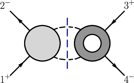
Refer to caption

(a)

Refer to caption

(b)

Figure 5: The (12)-channel (a) and (34)-channel (b) unitary cuts which determine the renormalization of 𝒪(ψ4)1\mathcal{O}_{{(\psi^{4})_{1}}} by 𝒪(D2​φ4)1\mathcal{O}_{{(D^{2}\varphi^{4})_{1}}} or 𝒪(D2​φ4)2\mathcal{O}_{{(D^{2}\varphi^{4})_{2}}}. The (23)- and (14)-channel cuts are given by the exchange of legs 2 and 4. In each, the darker blobs indicate a higher-dimension operator insertion, and the vertical (blue) dashed line indicates the integral over phase space of the particles crossing the cut.

Next, consider the case 𝒪(ψ4)1←𝒪(D2​φ4)2\mathcal{O}_{{(\psi^{4})_{1}}}\leftarrow\mathcal{O}_{{(D^{2}\varphi^{4})_{2}}}, which we also show has a zero entry in the anomalous dimension matrix of our simplified model. We organize the calculation into the three types of cuts as in the previous case, with the only difference being that, in case (3), the one-loop amplitude with an insertion of 𝒪(D2​φ4)2\mathcal{O}_{{(D^{2}\varphi^{4})_{2}}}, and with two scalars and two fermions as external particles is nonzero, and in fact has a UV divergence. While the presence of nonzero cuts, shown diagrammatically in Figure 5, might seem to imply that the two-loop anomalous dimension must be nonzero, we will show that it actually evaluates to zero as well.

Using the external state ⟨12+ψ 3−ψ¯4+ψ|−ψ¯\langle{1{}_{\vphantom{\overline{\psi}}\psi}^{+}}{2{}_{\,\overline{\psi}}^{-}\,}{3{}_{\vphantom{\overline{\psi}}\psi}^{+}}{4{}_{\,\overline{\psi}}^{-}\,}| and setting 𝒪i=𝒪(D2​φ4)2\mathcal{O}_{i}=\mathcal{O}_{{(D^{2}\varphi^{4})_{2}}}, Eq. (37) reduces to

γψ4←(D2​φ4)2UV⁡(2)​Fψ4(0)+γ(D​φ2​ψ2)2←(D2​φ4)2UV⁡(1)​F(D​φ2​ψ2)2(1)\displaystyle\gamma^{\rm UV(2)}_{\psi^{4}\leftarrow{(D^{2}\varphi^{4})_{2}}}F_{\psi^{4}}^{(0)}+\gamma^{\rm UV(1)}_{{(D\varphi^{2}\psi^{2})_{2}}\leftarrow{(D^{2}\varphi^{4})_{2}}}F_{{(D\varphi^{2}\psi^{2})_{2}}}^{(1)} (45)
=−1π(ℳ2→212+ℳ2→214+ℳ2→223+ℳ2→234)(0)⊗ReF(D2​φ4)2(1),\displaystyle\hskip 56.9055pt=-\frac{1}{\pi}(\mathcal{M}_{2\rightarrow 2}^{12}+\mathcal{M}_{2\rightarrow 2}^{14}+\mathcal{M}_{2\rightarrow 2}^{23}+\mathcal{M}_{2\rightarrow 2}^{34})^{(0)}\otimes\text{Re}F_{{(D^{2}\varphi^{4})_{2}}}^{(1)}\,,

where on the right-hand side we only find cuts of the form in Figure 5 with an 𝒪(D2​φ4)2\mathcal{O}_{{(D^{2}\varphi^{4})_{2}}} insertion, and the (13) and (24) channels are not allowed. For instance the (12)-channel cut is

(ℳ2→212)(0)⊗Re​F(D2​φ4)2(1)\displaystyle(\mathcal{M}_{2\rightarrow 2}^{12})^{(0)}\otimes\text{Re}F_{{(D^{2}\varphi^{4})_{2}}}^{(1)} (46)
=2∫dLIPS2⟨12+ψ|−ψ¯ℳ|ℓ1ℓ2φ⟩φ¯(0)Re⟨ℓ1ℓ2φ 3φ¯4+ψ|−ψ¯𝒪(D2​φ4)2|0⟩(1).\displaystyle\hskip 28.45274pt=2\int d\text{LIPS}_{2}\,\langle{1{}_{\vphantom{\overline{\psi}}\psi}^{+}}{2{}_{\,\overline{\psi}}^{-}\,}|\mathcal{M}|\ell_{1}{}_{\vphantom{\overline{\phi}}\varphi}^{\vphantom{+}}\ell_{2}{}_{\,\vphantom{\overline{\phi}}\overline{\varphi}}^{\vphantom{+}}\,\rangle^{(0)}\,\text{Re}\langle\ell_{1}{}_{\vphantom{\overline{\phi}}\varphi}^{\vphantom{+}}\ell_{2}{}_{\,\vphantom{\overline{\phi}}\overline{\varphi}}^{\vphantom{+}}\,{3{}_{\vphantom{\overline{\psi}}\psi}^{+}}{4{}_{\,\overline{\psi}}^{-}\,}|\mathcal{O}_{{(D^{2}\varphi^{4})_{2}}}|0\rangle^{(1)}\,.

The factor of 2 is required to cancel the symmetry factor of 1/2 in our definition of the phase-space measure. Other terms in Eq. (37) drop out because 𝒪(D2​φ4)2\mathcal{O}_{{(D^{2}\varphi^{4})_{2}}} does not have either a one-loop or tree-level form factor with a four-fermion external state, and does not renormalize 𝒪(D​φ2​ψ2)1\mathcal{O}_{{(D\varphi^{2}\psi^{2})_{1}}} or the 𝒪ψ4\mathcal{O}_{\psi^{4}} operators at one loop. In particular, the β\beta-function also does not appear.

For simplicity, we set the off-shell momentum qq to zero, and Eq. (45) then reduces to

γψ4←(D2​φ4)2UV⁡(2)Aψ4(0)(12+ψ 3−ψ¯4+ψ)−ψ¯+γ(D​φ2​ψ2)2←(D2​φ4)2UV⁡(1)A(D​φ2​ψ2)2(1)(12+ψ 3−ψ¯4+ψ)−ψ¯\displaystyle\gamma^{\rm UV(2)}_{\psi^{4}\leftarrow{(D^{2}\varphi^{4})_{2}}}A_{\psi^{4}}^{(0)}({1{}_{\vphantom{\overline{\psi}}\psi}^{+}}{2{}_{\,\overline{\psi}}^{-}\,}{3{}_{\vphantom{\overline{\psi}}\psi}^{+}}{4{}_{\,\overline{\psi}}^{-}\,})+\gamma^{\rm UV(1)}_{{(D\varphi^{2}\psi^{2})_{2}}\leftarrow{(D^{2}\varphi^{4})_{2}}}A_{{(D\varphi^{2}\psi^{2})_{2}}}^{(1)}({1{}_{\vphantom{\overline{\psi}}\psi}^{+}}{2{}_{\,\overline{\psi}}^{-}\,}{3{}_{\vphantom{\overline{\psi}}\psi}^{+}}{4{}_{\,\overline{\psi}}^{-}\,}) (47)
=−2π∑∫dLIPS2A(0)(12+ψ−−ψ¯ℓ2−φℓ1)φ¯ReA(D2​φ4)2(1)(ℓ1ℓ2φ 3φ¯4+ψ)−ψ¯,\displaystyle\hskip 28.45274pt=-\frac{2}{\pi}\sum\int d\text{LIPS}_{2}\,A^{(0)}({1{}_{\vphantom{\overline{\psi}}\psi}^{+}}{2{}_{\,\overline{\psi}}^{-}\,}-\!\ell_{2}{}_{\vphantom{\overline{\phi}}\varphi}^{\vphantom{+}}-\!\ell_{1}{}_{\,\vphantom{\overline{\phi}}\overline{\varphi}}^{\vphantom{+}}\,)\text{Re}A_{{(D^{2}\varphi^{4})_{2}}}^{(1)}(\ell_{1}{}_{\vphantom{\overline{\phi}}\varphi}^{\vphantom{+}}\ell_{2}{}_{\,\vphantom{\overline{\phi}}\overline{\varphi}}^{\vphantom{+}}\,{3{}_{\vphantom{\overline{\psi}}\psi}^{+}}{4{}_{\,\overline{\psi}}^{-}\,})\,,

where the sum is over the available channels. The relevant tree and renormalized one-loop amplitudes needed to construct the cut are (including the color factors):

A(0)(12+ψ 3−ψ¯4φ)φ¯\displaystyle A^{(0)}({1{}_{\vphantom{\overline{\psi}}\psi}^{+}}{2{}_{\,\overline{\psi}}^{-}\,}3{}_{\vphantom{\overline{\phi}}\varphi}^{\vphantom{+}}4{}_{\,\vphantom{\overline{\phi}}\overline{\varphi}}^{\vphantom{+}}\,) =Ti2​i1a​Ti4​i3a​g2​⟨23⟩​[13]s,\displaystyle=T^{a}_{i_{2}i_{1}}T^{a}_{i_{4}i_{3}}\,g^{2}\frac{\langle 23\rangle[13]}{s}\,, (48)
A(D2​φ4)2(1)(12+ψ 3−ψ¯4φ)φ¯\displaystyle A^{(1)}_{{(D^{2}\varphi^{4})_{2}}}({1{}_{\vphantom{\overline{\psi}}\psi}^{+}}{2{}_{\,\overline{\psi}}^{-}\,}3{}_{\vphantom{\overline{\phi}}\varphi}^{\vphantom{+}}4{}_{\,\vphantom{\overline{\phi}}\overline{\varphi}}^{\vphantom{+}}\,) =Ti2​i1aTi4​i3ag~29⟨23⟩[13](3log(−s/μ2)+8),\displaystyle=T^{a}_{i_{2}i_{1}}T^{a}_{i_{4}i_{3}}\,\frac{\widetilde{g}^{2}}{9}\langle 23\rangle[13](3\log(-s/\mu^{2})+8)\,, (49)

where again the flavor indices have been dropped for simplicity. Note the form of Eq. (47) provides a nontrivial check on the phase space integral on the right-hand side: A(D2​φ4)2(1)A_{{(D^{2}\varphi^{4})_{2}}}^{(1)} contains terms proportional to log(−s/μ2)\log(-s/\mu^{2}), which, after the phase-space integral, must cancel against terms in A(D​φ2​ψ2)2(1)A_{{(D\varphi^{2}\psi^{2})_{2}}}^{(1)}.

We can readily evaluate the cut by relabeling the amplitudes (48)–(49) and applying the spinor parametrization (25) to the scalars crossing the cut. This yields an integral with no poles in z= ei​ϕz=\text{ e}^{i\phi}, other than the pole at zero. This can be seen by the fact that all spinor products in A(0)A^{(0)} are either proportional to  e±i​ϕ\text{ e}^{\pm i\phi} or else have no ϕ\phi dependence under our parametrization, whereas A(D2​φ4)2(1)A_{{(D^{2}\varphi^{4})_{2}}}^{(1)} only has a pole in ss. This makes the ϕ\phi integral trivial to evaluate, resulting in:

∫0π2dθg~418⟨24⟩[13]sin3(2θ)(3log(−s/μ2)+8)Ti2​i1aTi4​i3a\displaystyle\int_{0}^{\frac{\pi}{2}}d\theta\,\frac{\widetilde{g}^{4}}{18}\langle 24\rangle[13]\sin^{3}(2\theta)(3\log(-s/\mu^{2})+8)T^{a}_{i_{2}i_{1}}T^{a}_{i_{4}i_{3}}
=g~427⟨24⟩[13](3log(−s/μ2)+8)Ti2​i1aTi4​i3a,\displaystyle\hskip 170.71652pt=\frac{\widetilde{g}^{4}}{27}\langle 24\rangle[13](3\log(-s/\mu^{2})+8)T^{a}_{i_{2}i_{1}}T^{a}_{i_{4}i_{3}}\,, (50)

for the (12)-channel cut. The (34)-channel cut gives the same result, while the other cuts yield the same result with legs two and four exchanged. Summing over the three other channels, we exactly match the second term on the left-hand side of Eq. (45), since γ(D​φ2​ψ2)2←(D2​φ4)2UV⁡(1)=g~2/3\gamma^{\rm UV(1)}_{{(D\varphi^{2}\psi^{2})_{2}}\leftarrow{(D^{2}\varphi^{4})_{2}}}=\widetilde{g}^{2}/3 and

A(D​φ2​ψ2)2(1)\displaystyle A_{{(D\varphi^{2}\psi^{2})_{2}}}^{(1)} =2​g~29⟨24⟩[13](3log(−s/μ2)+8)Ti2​i1aTi4​i3a−(2↔4).\displaystyle=\frac{2\widetilde{g}^{2}}{9}\langle 24\rangle[13](3\log(-s/\mu^{2})+8)T^{a}_{i_{2}i_{1}}T^{a}_{i_{4}i_{3}}-(2\leftrightarrow 4)\,. (51)

Therefore the cuts exactly cancel all terms on the left-hand side of Eq. (45) involving the one-loop anomalous dimensions and form-factors, leaving γψ4←(D2​φ4)2UV⁡(2)​Fψ4(0)=0\gamma^{\rm UV(2)}_{\psi^{4}\leftarrow{(D^{2}\varphi^{4})_{2}}}F^{(0)}_{\psi^{4}}=0. Thus the two-loop anomalous dimension γψ4←(D2​φ4)2UV⁡(2)\gamma^{\rm UV(2)}_{\psi^{4}\leftarrow{(D^{2}\varphi^{4})_{2}}} is zero.

In fact, we could have come to this conclusion simply by examining the form of the one-loop amplitudes in Eqs.  (49) and (51). First, note the two-loop anomalous dimension must be g~4\widetilde{g}^{4} times a number (i.e., it does not have any kinematic dependence). Logarithmic terms resulting from the cut on the right-hand side of (45) must therefore cancel against logarithmic terms in A(D​φ2​ψ2)2(1)A^{(1)}_{{(D\varphi^{2}\psi^{2})_{2}}}. Since both one-loop form factors are proportional to the factor (3log(−s/μ2)+8)(3\log(-s/\mu^{2})+8), and since this term can be pulled out of the phase-space integral on the right-hand side of Eq. (45), the cancellation of the logarithmic terms implies cancellation of the rational term as well. Thus, even though there are nonzero cuts, there can be no remaining rational term that leads to a nonzero two-loop anomalous dimension.

At this point, the vanishing of the two-loop anomalous dimensions due to the cancellation of one-loop rational terms might seem accidental. However, one must remember that such local rational pieces are scheme dependent and can be adjusted by adding finite local counter-terms. As described in Section 3, the rational terms of both one-loop amplitudes in (49) and (51) can be set to zero by such finite counterterms, which would also result in γψ4←(D2​φ4)2UV⁡(2)=0\gamma^{\rm UV(2)}_{\psi^{4}\leftarrow{(D^{2}\varphi^{4})_{2}}}=0. For this particular example, it just so happened that the naive MS¯\overline{\rm MS} scheme has zero anomalous dimension, but next we will see that this is not always the case.

As a cross-check, we have verified that the Eq. (32) is also satisfied. The crucial substitution log(−s/μ2)→log(−s/μ2)−iπ\log(-s/\mu^{2})\rightarrow\log(-s/\mu^{2})-i\pi, is required in the right-hand side of that equation, coming from the analytic continuation of the amplitude from the Euclidean region to the correct physical region, which must be carried out for use in Eqs. (2.3)–(31).

4.2.2 𝒪D2​φ4←𝒪(ψ4)1\mathcal{O}_{D^{2}\varphi^{4}}\leftarrow\mathcal{O}_{{(\psi^{4})_{1}}}

Refer to caption

(a)

Refer to caption

(b)

Figure 6: The (a) (12)-channel and (b) (34)-channel unitary cuts which determine the renormalization of 𝒪(D2​φ4)1\mathcal{O}_{{(D^{2}\varphi^{4})_{1}}} and 𝒪(D2​φ4)2\mathcal{O}_{{(D^{2}\varphi^{4})_{2}}} by 𝒪(ψ4)1\mathcal{O}_{{(\psi^{4})_{1}}} or 𝒪(ψ4)2\mathcal{O}_{{(\psi^{4})_{2}}}. The (23)- and (14)-channel cuts are given by exchanging legs 2 and 4. In each, the darker blobs indicate a higher-dimension operator insertion, and the vertical (blue) dashed line indicates the integral over phase space of the particles crossing the cut.

This section will provide our first example of nonzero two-loop anomalous dimension matrix elements in MS¯\overline{\rm MS}, while demonstrating how an appropriate choice of scheme, i.e. choice of finite local counterterms, can eliminate the two-loop anomalous dimensions of this example.

We will begin with the calculation in MS¯\overline{\rm MS}. Again, there is no three-particle cut, due to the particle content of the two types of operators in question. Using the external state ⟨12φ 3φ¯4φ|φ¯\langle 1{}_{\vphantom{\overline{\phi}}\varphi}^{\vphantom{+}}2{}_{\,\vphantom{\overline{\phi}}\overline{\varphi}}^{\vphantom{+}}\,3{}_{\vphantom{\overline{\phi}}\varphi}^{\vphantom{+}}4{}_{\,\vphantom{\overline{\phi}}\overline{\varphi}}^{\vphantom{+}}\,| and setting 𝒪i→𝒪(ψ4)1\mathcal{O}_{i}\rightarrow\mathcal{O}_{{(\psi^{4})_{1}}}, Eq. (37) becomes

γ(D2​φ4)1←(ψ4)1UV⁡(2)​F(D2​φ4)1(0)+γ(D2​φ4)2←(ψ4)1UV⁡(2)​F(D2​φ4)2(0)+γ(D​φ2​ψ2)2←(ψ4)1UV⁡(1)​F(D​φ2​ψ2)2(1)\displaystyle\gamma^{\rm UV(2)}_{{(D^{2}\varphi^{4})_{1}}\leftarrow{(\psi^{4})_{1}}}F^{(0)}_{{(D^{2}\varphi^{4})_{1}}}+\gamma^{\rm UV(2)}_{{(D^{2}\varphi^{4})_{2}}\leftarrow{(\psi^{4})_{1}}}F^{(0)}_{{(D^{2}\varphi^{4})_{2}}}+\gamma^{\rm UV(1)}_{{(D\varphi^{2}\psi^{2})_{2}}\leftarrow{(\psi^{4})_{1}}}F^{(1)}_{{(D\varphi^{2}\psi^{2})_{2}}} (52)
=−1π(ℳ2→212+ℳ2→214+ℳ2→223+ℳ2→234)(0)⊗ReF(ψ4)1(1).\displaystyle\hskip 113.81102pt=-\frac{1}{\pi}(\mathcal{M}_{2\rightarrow 2}^{12}+\mathcal{M}_{2\rightarrow 2}^{14}+\mathcal{M}_{2\rightarrow 2}^{23}+\mathcal{M}_{2\rightarrow 2}^{34})^{(0)}\otimes\text{Re}F_{{(\psi^{4})_{1}}}^{(1)}\,.

As for the previous example, the logarithmic terms in the cuts must cancel against terms in the amplitude F(D​φ2​ψ2)2(1)F^{(1)}_{{(D\varphi^{2}\psi^{2})_{2}}} on the left-hand side of the equation. Since we are dealing with four-point matrix elements we will again set q=0q=0. Then the one-loop amplitudes required for this example are

A(ψ4)1(1)(12+ψ 3−ψ¯4φ)φ¯\displaystyle A^{(1)}_{{(\psi^{4})_{1}}}({1{}_{\vphantom{\overline{\psi}}\psi}^{+}}{2{}_{\,\overline{\psi}}^{-}\,}3{}_{\vphantom{\overline{\phi}}\varphi}^{\vphantom{+}}4{}_{\,\vphantom{\overline{\phi}}\overline{\varphi}}^{\vphantom{+}}\,) =2​g~29⟨23⟩[13](3log(−s/μ2)−2)Ti2​i1aTi4​i3a,\displaystyle=\frac{2\widetilde{g}^{2}}{9}\langle 23\rangle[13](3\log(-s/\mu^{2})-2)T^{a}_{i_{2}i_{1}}T^{a}_{i_{4}i_{3}}\,, (53)
A(D​φ2​ψ2)2(1)(12φ 3φ¯4φ)φ¯\displaystyle A^{(1)}_{{(D\varphi^{2}\psi^{2})_{2}}}(1{}_{\vphantom{\overline{\phi}}\varphi}^{\vphantom{+}}2{}_{\,\vphantom{\overline{\phi}}\overline{\varphi}}^{\vphantom{+}}\,3{}_{\vphantom{\overline{\phi}}\varphi}^{\vphantom{+}}4{}_{\,\vphantom{\overline{\phi}}\overline{\varphi}}^{\vphantom{+}}\,) =2​g~29(t−u)(3log(−s/μ2)−5)Ti2​i1aTi4​i3a+(2↔4),\displaystyle=\frac{2\widetilde{g}^{2}}{9}(t-u)(3\log(-s/\mu^{2})-5)T^{a}_{i_{2}i_{1}}T^{a}_{i_{4}i_{3}}+(2\leftrightarrow 4)\,, (54)

and the tree-level amplitudes needed are in Eq. (48) along with

A(D2​φ4)1(0)(12φ 3φ¯4φ)φ¯\displaystyle A_{{(D^{2}\varphi^{4})_{1}}}^{(0)}(1{}_{\vphantom{\overline{\phi}}\varphi}^{\vphantom{+}}2{}_{\,\vphantom{\overline{\phi}}\overline{\varphi}}^{\vphantom{+}}\,3{}_{\vphantom{\overline{\phi}}\varphi}^{\vphantom{+}}4{}_{\,\vphantom{\overline{\phi}}\overline{\varphi}}^{\vphantom{+}}\,) =t​δi2​i1​δi4​i3+s​δi4​i1​δi2​i3,\displaystyle=\;t\delta_{i_{2}i_{1}}\delta_{i_{4}i_{3}}+s\delta_{i_{4}i_{1}}\delta_{i_{2}i_{3}}\,, (55)
A(D2​φ4)2(0)(12φ 3φ¯4φ)φ¯\displaystyle A_{{(D^{2}\varphi^{4})_{2}}}^{(0)}(1{}_{\vphantom{\overline{\phi}}\varphi}^{\vphantom{+}}2{}_{\,\vphantom{\overline{\phi}}\overline{\varphi}}^{\vphantom{+}}\,3{}_{\vphantom{\overline{\phi}}\varphi}^{\vphantom{+}}4{}_{\,\vphantom{\overline{\phi}}\overline{\varphi}}^{\vphantom{+}}\,) = 2​s​δi2​i1​δi4​i3+2​t​δi4​i1​δi2​i3,\displaystyle=\;2s\delta_{i_{2}i_{1}}\delta_{i_{4}i_{3}}+2t\delta_{i_{4}i_{1}}\delta_{i_{2}i_{3}}\,, (56)

which are shown in a slightly different basis of color factors than those shown in the appendix. The phase-space integral is evaluated in the same manner as the previous examples, with the result of the (12)-channel cut being

−1π\displaystyle-\frac{1}{\pi} ∫dLIPS2∑h1,h2A(0)(12φ−φ¯ℓ1−h1ψℓ2)h2ψ¯A(ψ4)1(1)(ℓ2ℓ1h2ψ 3h1ψ¯4φ)φ¯\displaystyle\int d\text{LIPS}_{2}\,\sum_{h_{1},h_{2}}A^{(0)}(1{}_{\vphantom{\overline{\phi}}\varphi}^{\vphantom{+}}2{}_{\,\vphantom{\overline{\phi}}\overline{\varphi}}^{\vphantom{+}}\,{-\ell_{1}{}_{\vphantom{\overline{\psi}}\psi}^{h_{1}}}\,{-\ell_{2}{}_{\,\overline{\psi}}^{h_{2}}\,})A^{(1)}_{{(\psi^{4})_{1}}}({\ell_{2}{}_{\vphantom{\overline{\psi}}\psi}^{h_{2}}}\,{\ell_{1}{}_{\,\overline{\psi}}^{h_{1}}\,}3{}_{\vphantom{\overline{\phi}}\varphi}^{\vphantom{+}}4{}_{\,\vphantom{\overline{\phi}}\overline{\varphi}}^{\vphantom{+}}\,)
=−227g~4(t−u)(3log(−s/μ2)−2)Ti2​i1aTi4​i3a.\displaystyle\hskip 85.35826pt=-\frac{2}{27}\widetilde{g}^{4}(t-u)(3\log(-s/\mu^{2})-2)T^{a}_{i_{2}i_{1}}T^{a}_{i_{4}i_{3}}\,. (57)

After summing over all channels and subtracting the contribution of γ(D​φ2​ψ2)2←(ψ4)1UV⁡(1)​F(D​φ2​ψ2)2(1)\gamma^{\rm UV(1)}_{{(D\varphi^{2}\psi^{2})_{2}}\leftarrow{(\psi^{4})_{1}}}F^{(1)}_{{(D\varphi^{2}\psi^{2})_{2}}} in Eq. (52)—thus canceling the logarithmic terms—the two-loop anomalous dimensions are given by

γ(D2​φ4)1←(ψ4)1UV⁡(2)​(CLOSE\displaystyle\gamma^{\rm UV(2)}_{{(D^{2}\varphi^{4})_{1}}\leftarrow{(\psi^{4})_{1}}}( OPENt​δi2​i1​δi4​i3+s​δ41​δ23)+γ(D2​φ4)2←(ψ4)1UV⁡(2)​(2​s​δi2​i1​δi4​i3+2​t​δi4​i1​δi2​i3)\displaystyle t\delta_{i_{2}i_{1}}\delta_{i_{4}i_{3}}+s\delta_{41}\delta_{23})+\gamma^{\rm UV(2)}_{{(D^{2}\varphi^{4})_{2}}\leftarrow{(\psi^{4})_{1}}}(2s\delta_{i_{2}i_{1}}\delta_{i_{4}i_{3}}+2t\delta_{i_{4}i_{1}}\delta_{i_{2}i_{3}}) (58)
=\displaystyle= −49​g~4​(t−u)​Ti2​i1a​Ti4​i3a+(2↔4).\displaystyle-\frac{4}{9}\widetilde{g}^{4}(t-u)T^{a}_{i_{2}i_{1}}T^{a}_{i_{4}i_{3}}+(2\leftrightarrow 4)\,.

Applying the color Fierz identity,

Ti​ja​Tk​la=δi​l​δk​j−1N​δi​j​δk​l,T^{a}_{ij}T^{a}_{kl}=\delta_{il}\delta_{kj}-\frac{1}{N}\delta_{ij}\delta_{kl}\,, (59)

and solving for the two-loop anomalous dimensions, we find

γ(D2​φ4)1←(ψ4)1UV⁡(2)=\displaystyle\gamma^{\rm UV(2)}_{{(D^{2}\varphi^{4})_{1}}\leftarrow{(\psi^{4})_{1}}}= −4​g~4​(N−2)9​N,\displaystyle\hbox{}-\frac{4\widetilde{g}^{4}(N-2)}{9N}\,,
γ(D2​φ4)1←(ψ4)2UV⁡(2)=\displaystyle\gamma^{\rm UV(2)}_{{(D^{2}\varphi^{4})_{1}}\leftarrow{(\psi^{4})_{2}}}= ​2​g~4​(2​N−1)9​N,\displaystyle\hbox{}\frac{2\widetilde{g}^{4}(2N-1)}{9N}\,, (60)

in the MS¯\overline{\rm MS} scheme. Although these anomalous dimension matrix elements are nonzero in the MS¯\overline{\rm MS} scheme, a simple rational shift of the coefficients c(D2​φ4)1,c(D2​φ4)2c_{{(D^{2}\varphi^{4})_{1}}},c_{{(D^{2}\varphi^{4})_{2}}}, and c(D​φ2​ψ2)2c_{{(D\varphi^{2}\psi^{2})_{2}}} can set them to zero. This is accomplished by the following shifts in the coefficients:

c(D2​φ4)1⟶c~(D2​φ4)1=c(D2​φ4)1+10​g~2​(N−2)9​N​c(D​φ2​ψ2)2,c(D2​φ4)2⟶c~(D2​φ4)2=c(D2​φ4)2+5​g~2​(2​N−1)9​N​c(D​φ2​ψ2)2,c(D​φ2​ψ2)2⟶c~(D​φ2​ψ2)2=c(D​φ2​ψ2)2−2​g~29​c(ψ4)1,\displaystyle\begin{split}c_{{(D^{2}\varphi^{4})_{1}}}\longrightarrow&\,\widetilde{c}_{{(D^{2}\varphi^{4})_{1}}}=c_{{(D^{2}\varphi^{4})_{1}}}+\frac{10\widetilde{g}^{2}(N-2)}{9N}c_{{(D\varphi^{2}\psi^{2})_{2}}}\,,\\ c_{{(D^{2}\varphi^{4})_{2}}}\longrightarrow&\,\widetilde{c}_{{(D^{2}\varphi^{4})_{2}}}=c_{{(D^{2}\varphi^{4})_{2}}}+\frac{5\widetilde{g}^{2}(2N-1)}{9N}c_{{(D\varphi^{2}\psi^{2})_{2}}}\,,\\ c_{{(D\varphi^{2}\psi^{2})_{2}}}\longrightarrow&\,\widetilde{c}_{{(D\varphi^{2}\psi^{2})_{2}}}=c_{{(D\varphi^{2}\psi^{2})_{2}}}-\frac{2\widetilde{g}^{2}}{9}c_{{(\psi^{4})_{1}}}\,,\end{split} (61)

which yields

γ~(D2​φ4)1←(ψ4)1UV⁡(2)=0,γ~(D2​φ4)2←(ψ4)1UV⁡(2)=0,\displaystyle\widetilde{\gamma}^{\rm UV(2)}_{{(D^{2}\varphi^{4})_{1}}\leftarrow{(\psi^{4})_{1}}}=0\,,\hskip 56.9055pt\widetilde{\gamma}^{\rm UV(2)}_{{(D^{2}\varphi^{4})_{2}}\leftarrow{(\psi^{4})_{1}}}=0\,, (62)

where the tilde indicates the modified scheme. The shifts above are equivalent to a finite renormalization of the operator at one loop. Generally this can be achieved by choosing the rational terms in γ(D​φ2​ψ2)2←(ψ4)1UV⁡(1)​F(D​φ2​ψ2)2(1)\gamma^{\rm UV(1)}_{{(D\varphi^{2}\psi^{2})_{2}}\leftarrow{(\psi^{4})_{1}}}F^{(1)}_{{(D\varphi^{2}\psi^{2})_{2}}} to match those of the cuts. In our particular example we set the rational terms of both (53) and (54) to zero. We briefly comment below on the consequences of this redefinition for the two-loop RG running of the operators involved.

While we do not present the analogous calculation for 𝒪(ψ4)2\mathcal{O}_{{(\psi^{4})_{2}}} here, by inspecting Table 3, we can deduce that the two-loop anomalous dimensions γ(D2​φ4)1←(ψ4)2UV⁡(2)\gamma^{\rm UV(2)}_{{(D^{2}\varphi^{4})_{1}}\leftarrow{(\psi^{4})_{2}}} and γ(D2​φ4)2←(ψ4)2UV⁡(2)\gamma^{\rm UV(2)}_{{(D^{2}\varphi^{4})_{2}}\leftarrow{(\psi^{4})_{2}}} can also be set to zero with the appropriate choice of finite counterterms.

4.2.3 General comments about scheme redefinition

As mentioned above, the scheme choice that sets some two-loop anomalous dimensions to zero is equivalent to a finite renormalization of the operators

𝒪~i=Zi​jfin​Oj,whereZi​jfin=δi​j+fi​j​(g(4)),\widetilde{\mathcal{O}}_{i}=Z^{\rm fin}_{ij}O_{j}\,,\quad\text{where}\quad Z^{\rm fin}_{ij}=\delta_{ij}+f_{ij}(g^{(4)})\,, (63)

and the quantity fi​jf_{ij} is finite and has a perturbative expansion starting at one loop, fi​j​(g(4))=fi​j(1)+⋯f_{ij}(g^{(4)})=f_{ij}^{(1)}+\cdots. As usual, the redefinition of the coefficients, c~i=Zi​jfin⁡(c)​cj\widetilde{c}_{i}=Z^{{\rm fin}\,(c)}_{ij}c_{j} is given by the inverse, Zi​jfin⁡(c)=(Zi​jfin)−1Z^{{\rm fin}\,(c)}_{ij}=(Z^{\rm fin}_{ij})^{-1}. The effect of such a scheme redefinition can be easily analyzed using the unitarity-based formalism employed in this paper. Since the coupling dependence of fi​jf_{ij} starts at one loop we have that

F~i(0)\displaystyle\widetilde{F}^{(0)}_{i} =Fi(0),\displaystyle=F^{(0)}_{i}\,, (64)
F~i(1)\displaystyle\widetilde{F}^{(1)}_{i} =Fi(1)+fi​j(1)​Fj(0),\displaystyle=F^{(1)}_{i}+f^{(1)}_{ij}F^{(0)}_{j}\,, (65)

where the tilde indicates a form factor of the redefined operator 𝒪~i\widetilde{\mathcal{O}}_{i}. From Eqs. (64) and (22) we conclude the one-loop anomalous dimensions are unaffected by the finite renormalization, i.e., Δ~​γi​j(1)=Δ​γi​j(1)\widetilde{\Delta}\gamma^{(1)}_{ij}=\Delta\gamma^{(1)}_{ij}. Similarly, writing Eq. (37) for the redefined operator

[Δγ~i​j(1)+δi​jβ(1)∂]ReF~j(1)\displaystyle\left[\Delta\widetilde{\gamma}^{(1)}_{ij}+\delta_{ij}\beta^{(1)}\partial\right]\text{Re}\widetilde{F}_{j}^{(1)} +[Δγ~i​j(2)+δi​jβ(2)∂]F~j(0)=−1π[Re(ℳ)Re(F~i)](2).\displaystyle+\left[\Delta\widetilde{\gamma}^{(2)}_{ij}+\delta_{ij}\beta^{(2)}\partial\right]\widetilde{F}_{j}^{(0)}=-\frac{1}{\pi}\left[\text{Re}(\mathcal{M})\text{Re}(\widetilde{F}_{i})\right]^{(2)}. (66)

and using Eqs. (64) and (65) together with Eqs. (22) and  (37), while keeping in mind that the infrared anomalous dimensions are not changed by redefining the scheme, we find the relation between the two-loop anomalous dimensions in the two schemes,

γ~i​jUV⁡(2)=γi​jUV⁡(2)+fi​k(1)​γk​jUV⁡(1)−γi​kUV⁡(1)​fk​j(1)−β(1)​∂fi​j(1).\widetilde{\gamma}^{\rm UV(2)}_{ij}=\gamma^{\rm UV(2)}_{ij}+f^{(1)}_{ik}\gamma^{\rm UV(1)}_{kj}-\gamma^{\rm UV(1)}_{ik}f^{(1)}_{kj}-\beta^{(1)}\partial f^{(1)}_{ij}\,. (67)

In general, one would like to solve this equation for fi​k(1)f^{(1)}_{ik} to get as many vanishing entries as possible in γ~i​jUV⁡(2)\widetilde{\gamma}^{\rm UV(2)}_{ij}.

We have explicitly verified Eq. (67) in the examples above, where we set the anomalous dimensions of the form γ~D2​φ4←ψ4UV⁡(2)\widetilde{\gamma}^{\rm UV(2)}_{D^{2}\varphi^{4}\leftarrow\psi^{4}} to zero by appropriately choosing fD​φ2​ψ2←ψ4(1)f^{(1)}_{D\varphi^{2}\psi^{2}\leftarrow\psi^{4}} and fD2​φ4←D​φ2​ψ4(1)f^{(1)}_{D^{2}\varphi^{4}\leftarrow D\varphi^{2}\psi^{4}}. In addition, fD2​φ4←ψ4(1)f^{(1)}_{D^{2}\varphi^{4}\leftarrow\psi^{4}} vanished, which from Eq. (67) implies the the absence of a term induced by the β\beta-function in the new two-loop anomalous dimension. On the other hand, it is clear from Eq. (67) that the finite renormalizations will induce some additional running in the two-loop anomalous dimensions γ~D​φ2​ψ2←ψ4UV⁡(2)\widetilde{\gamma}^{\rm UV(2)}_{D\varphi^{2}\psi^{2}\leftarrow\psi^{4}} and γ~D2​φ4←D​φ2​ψ4UV⁡(2)\widetilde{\gamma}^{\rm UV(2)}_{D^{2}\varphi^{4}\leftarrow D\varphi^{2}\psi^{4}}, proportional to the one-loop beta function and ∂f(1)\partial f^{(1)}. However, this additional running is harmless, since those operators already mix at one loop. Furthermore, the corresponding entries in the two-loop anomalous-dimension matrix receive contributions from both two- and three-particle cuts that have no a priori reason to vanish, so we expect them in any case to run. In summary, our scheme choice prevents certain operators from mixing at two-loops at the expense of modifying the running of operators that, in any case, mix at one loop in the original scheme.

4.3 Zeros from color selection rules
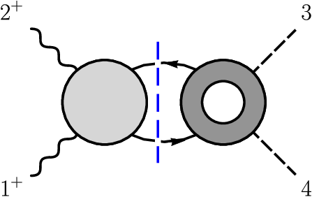
Refer to caption

(a)

Refer to caption

(b)

Figure 7: (12)-channel (a) and (34)-channel (b) unitary cuts which determine the renormalization of 𝒪(φ2​F2)1\mathcal{O}_{{(\varphi^{2}F^{2})_{1}}} and 𝒪(φ2​F2)2\mathcal{O}_{{(\varphi^{2}F^{2})_{2}}} by 𝒪(ψ4)1\mathcal{O}_{{(\psi^{4})_{1}}} or 𝒪(ψ4)2\mathcal{O}_{{(\psi^{4})_{2}}}. There are no t-channel cuts for this process. In each diagram, the darker blobs indicate a higher-dimension operator insertion, and the dashed line indicates the integral over phase space of the particles crossing the cut.

This section will provide an example of another type of selection rule, wherein a mismatch between the color of the cuts and the color of the target operators prevents renormalization at two loops.

4.3.1 𝒪φ2​F2←𝒪ψ4\mathcal{O}_{\varphi^{2}F^{2}}\leftarrow\mathcal{O}_{\psi^{4}}

For this example we choose the external state to be ⟨1​2φ​ 3+φ¯​4+|\langle 1{}_{\vphantom{\overline{\phi}}\varphi}^{\vphantom{+}}2{}_{\,\vphantom{\overline{\phi}}\overline{\varphi}}^{\vphantom{+}}\,3^{+}4^{+}|, under which both 𝒪(φ2​F2)1\mathcal{O}_{{(\varphi^{2}F^{2})_{1}}} and 𝒪(φ2​F2)2\mathcal{O}_{{(\varphi^{2}F^{2})_{2}}} are nonzero. Using this state and setting 𝒪i→𝒪(ψ4)1\mathcal{O}_{i}\rightarrow\mathcal{O}_{{(\psi^{4})_{1}}}, Eq. (37) reduces to

γ(φ2​F2)1←(ψ4)1UV⁡(2)\displaystyle\gamma^{\rm UV(2)}_{{(\varphi^{2}F^{2})_{1}}\leftarrow{(\psi^{4})_{1}}} F(φ2​F2)1(0)+γ(φ2​F2)2←(ψ4)1UV⁡(2)​F(φ2​F2)2(0)+γ(D​φ2​ψ2)2←(ψ4)1UV⁡(1)​F(D​φ2​ψ2)2(1)\displaystyle F^{(0)}_{{(\varphi^{2}F^{2})_{1}}}+\gamma^{\rm UV(2)}_{{(\varphi^{2}F^{2})_{2}}\leftarrow{(\psi^{4})_{1}}}F^{(0)}_{{(\varphi^{2}F^{2})_{2}}}+\gamma^{\rm UV(1)}_{{(D\varphi^{2}\psi^{2})_{2}}\leftarrow{(\psi^{4})_{1}}}F^{(1)}_{{(D\varphi^{2}\psi^{2})_{2}}} (68)
=−1π​((ℳ2→212)(0)⊗Re​F(ψ4)1(1)+(ℳ2→234)(0)⊗Re​F(ψ4)1(1)).\displaystyle\hskip 28.45274pt=-\frac{1}{\pi}\Big((\mathcal{M}_{2\rightarrow 2}^{12})^{(0)}\otimes\text{Re}F_{{(\psi^{4})_{1}}}^{(1)}+(\mathcal{M}_{2\rightarrow 2}^{34})^{(0)}\otimes\text{Re}F_{{(\psi^{4})_{1}}}^{(1)}\Big)\,.

Naively there would be the additional term γF3←(ψ4)1UV⁡(2)​FF3(0)\gamma^{\rm UV(2)}_{{F^{3}}\leftarrow{(\psi^{4})_{1}}}F^{(0)}_{{F^{3}}} on the left-hand-side of the equation, since 𝒪F3\mathcal{O}_{F^{3}} produces a nonzero tree amplitude with the state ⟨1​2φ​ 3+φ¯​4+|\langle 1{}_{\vphantom{\overline{\phi}}\varphi}^{\vphantom{+}}2{}_{\,\vphantom{\overline{\phi}}\overline{\varphi}}^{\vphantom{+}}\,3^{+}4^{+}|. However, as was discussed in Section 4.1, the length and particle content of 𝒪(ψ4)1\mathcal{O}_{{(\psi^{4})_{1}}} requires γF3←(ψ4)1UV⁡(2)=0\gamma^{\rm UV(2)}_{{F^{3}}\leftarrow{(\psi^{4})_{1}}}=0. Setting q=0q=0, the (12)-channel cut of the above equation is

(ℳ2→212)(0)⊗ReF(ψ4)1(1)=∫dLIPS2∑h1,h2A(0)(12φ−φ¯ℓ1−h1ψℓ2)−h2ψ¯A(ψ4)1(1)(ℓ2ℓ1h2ψ 3+h1ψ¯4+),\displaystyle(\mathcal{M}_{2\rightarrow 2}^{12})^{(0)}\otimes\text{Re}F_{{(\psi^{4})_{1}}}^{(1)}=\int d\text{LIPS}_{2}\,\sum_{h_{1},h_{2}}A^{(0)}(1{}_{\vphantom{\overline{\phi}}\varphi}^{\vphantom{+}}2{}_{\,\vphantom{\overline{\phi}}\overline{\varphi}}^{\vphantom{+}}\,{-\ell_{1}{}_{\vphantom{\overline{\psi}}\psi}^{h_{1}}}\,{-\ell_{2}{}_{\,\overline{\psi}}^{-h_{2}}\,})A^{(1)}_{{(\psi^{4})_{1}}}({\ell_{2}{}_{\vphantom{\overline{\psi}}\psi}^{h_{2}}}\,{\ell_{1}{}_{\,\overline{\psi}}^{h_{1}}\,}3^{+}4^{+})\,, (69)

and the (34)-channel cut is

(ℳ2→234)(0)⊗ReF(ψ4)1(1)=∫dLIPS2∑h1,h2A(0)(3+4+−ℓ1−h1ψℓ2)h2ψ¯A(ψ4)1(1)(ℓ2ℓ1h2ψ 1h1ψ¯2φ)φ¯.\displaystyle(\mathcal{M}_{2\rightarrow 2}^{34})^{(0)}\otimes\text{Re}F_{{(\psi^{4})_{1}}}^{(1)}=\int d\text{LIPS}_{2}\,\sum_{h_{1},h_{2}}A^{(0)}(3^{+}4^{+}{-\ell_{1}{}_{\vphantom{\overline{\psi}}\psi}^{h_{1}}}\,{-\ell_{2}{}_{\,\overline{\psi}}^{h_{2}}\,})A^{(1)}_{{(\psi^{4})_{1}}}({\ell_{2}{}_{\vphantom{\overline{\psi}}\psi}^{h_{2}}}\,{\ell_{1}{}_{\,\overline{\psi}}^{h_{1}}\,}1{}_{\vphantom{\overline{\phi}}\varphi}^{\vphantom{+}}2{}_{\,\vphantom{\overline{\phi}}\overline{\varphi}}^{\vphantom{+}}\,)\,. (70)

The (34)-channel cut vanishes, because the amplitude A(0)(3+4+−ℓ1−ψℓ2)ψ¯A^{(0)}(3^{+}4^{+}{-\ell_{1}{}_{\vphantom{\overline{\psi}}\psi}}\,{-\ell_{2}{}_{\,\overline{\psi}}\,}) is zero for all helicities of the fermions crossing the cut. This vanishing is required for the consistency of the logarithmic terms: A(ψ4)1(1)(ℓ2ℓ1h2ψ 1h1ψ¯2φ)φ¯A^{(1)}_{{(\psi^{4})_{1}}}({\ell_{2}{}_{\vphantom{\overline{\psi}}\psi}^{h_{2}}}\,{\ell_{1}{}_{\,\overline{\psi}}^{h_{1}}\,}1{}_{\vphantom{\overline{\phi}}\varphi}^{\vphantom{+}}2{}_{\,\vphantom{\overline{\phi}}\overline{\varphi}}^{\vphantom{+}}\,) includes a term proportional to log(−s/μ2)\log(-s/\mu^{2}), but there is no term on the left-hand side that can cancel it, since F(D​φ2​ψ2)2(1)​(1​2φ​ 3+φ¯​4+)F^{(1)}_{{(D\varphi^{2}\psi^{2})_{2}}}(1{}_{\vphantom{\overline{\phi}}\varphi}^{\vphantom{+}}2{}_{\,\vphantom{\overline{\phi}}\overline{\varphi}}^{\vphantom{+}}\,3^{+}4^{+}) is purely rational. The one-loop amplitudes needed for this calculation are

A(ψ4)1(1)​(1​ 2ψ+​ 3+ψ¯−​4+)\displaystyle A_{{(\psi^{4})_{1}}}^{(1)}({1{}_{\vphantom{\overline{\psi}}\psi}^{+}}\,{2{}_{\,\overline{\psi}}^{-}\,}3^{+}4^{+}) =−g~2​s​[14]​⟨24⟩​[Ta3,Ta4]i2​i13​⟨34⟩2,\displaystyle=-\frac{\widetilde{g}^{2}s[14]\langle 24\rangle\,[T^{a_{3}},T^{a_{4}}]_{i_{2}i_{1}}}{3\langle 34\rangle^{2}}\,, (71)
A(ψ4)1(1)​(1​ 2ψ−​ 3+ψ¯+​4+)\displaystyle A_{{(\psi^{4})_{1}}}^{(1)}({1{}_{\vphantom{\overline{\psi}}\psi}^{-}}\,{2{}_{\,\overline{\psi}}^{+}\,}3^{+}4^{+}) =−g~2​⟨12⟩​[23]​[24]​[Ta3,Ta4]i2​i13​⟨34⟩,\displaystyle=-\frac{\widetilde{g}^{2}\langle 12\rangle[23][24]\,[T^{a_{3}},T^{a_{4}}]_{i_{2}i_{1}}}{3\langle 34\rangle}\,, (72)
A(D​φ2​ψ2)2(1)​(1​2φ​ 3+φ¯​4+)\displaystyle A_{{(D\varphi^{2}\psi^{2})_{2}}}^{(1)}(1{}_{\vphantom{\overline{\phi}}\varphi}^{\vphantom{+}}2{}_{\,\vphantom{\overline{\phi}}\overline{\varphi}}^{\vphantom{+}}\,3^{+}4^{+}) =g~2​s​(t−u)​[Ta3,Ta4]i2​i13​⟨34⟩2,\displaystyle=\frac{\widetilde{g}^{2}s(t-u)\,[T^{a_{3}},T^{a_{4}}]_{i_{2}i_{1}}}{3\langle 34\rangle^{2}}\,, (73)

while the tree-level amplitudes needed for the cut calculation are (48) and its conjugate. The phase-space integrals are carried out in the same manner as the previous example, with the simplification that the functions are now entirely rational. The result of the phase-space integral is

−1π∫\displaystyle-\frac{1}{\pi}\int dLIPS2∑h1,h2A(0)(12φ−φ¯ℓ1−−h1ψℓ2)−h2ψ¯A(ψ4)1(1)(ℓ2ℓ1h2ψ 3+h1ψ¯4+)\displaystyle d\text{LIPS}_{2}\,\sum_{h_{1},h_{2}}A^{(0)}(1{}_{\vphantom{\overline{\phi}}\varphi}^{\vphantom{+}}2{}_{\,\vphantom{\overline{\phi}}\overline{\varphi}}^{\vphantom{+}}\,{-\ell_{1}{}_{\vphantom{\overline{\psi}}\psi}^{-h_{1}}}\,{-\ell_{2}{}_{\,\overline{\psi}}^{-h_{2}}\,})A^{(1)}_{{(\psi^{4})_{1}}}({\ell_{2}{}_{\vphantom{\overline{\psi}}\psi}^{h_{2}}}\,{\ell_{1}{}_{\,\overline{\psi}}^{h_{1}}\,}3^{+}4^{+})
=−2​g~4​s​(t−u)​[Ta3,Ta4]i2​i19​(⟨34⟩)2=γ(D​φ2​ψ2)2←(ψ4)1UV⁡(1)​A(D​φ2​ψ2)2(1).\displaystyle=-\frac{2\widetilde{g}^{4}s(t-u)\,[T^{a_{3}},T^{a_{4}}]_{i_{2}i_{1}}}{9(\langle 34\rangle)^{2}}=\gamma^{\rm UV(1)}_{{(D\varphi^{2}\psi^{2})_{2}}\leftarrow{(\psi^{4})_{1}}}A^{(1)}_{{(D\varphi^{2}\psi^{2})_{2}}}\,. (74)

Thus the phase-space integral exactly cancels against this term from the left-hand-side of Eq. (68), meaning the two-loop anomalous dimension is again zero.

Interestingly, this can also be seen without looking at the kinematic content of the cuts on the right-hand side of Eq. (68). Since the color of both 𝒪(φ2​F2)1\mathcal{O}_{{(\varphi^{2}F^{2})_{1}}} and 𝒪(φ2​F2)2\mathcal{O}_{{(\varphi^{2}F^{2})_{2}}} are symmetric in T3T^{3} and T4T^{4}, no combination of the two can produce the color factor [T3,T4]i2​i1[T^{3},T^{4}]_{i_{2}i_{1}}. Since this is the color of A(D​φ2​ψ2)2(1)​(1​2φ​ 3+φ¯​4+)A_{{(D\varphi^{2}\psi^{2})_{2}}}^{(1)}(1{}_{\vphantom{\overline{\phi}}\varphi}^{\vphantom{+}}2{}_{\,\vphantom{\overline{\phi}}\overline{\varphi}}^{\vphantom{+}}\,3^{+}4^{+}), and the color of A(ψ4)1(1)​(1​ 2ψ±​ 3+ψ¯∓​4+)A_{{(\psi^{4})_{1}}}^{(1)}({1{}_{\vphantom{\overline{\psi}}\psi}^{\pm}}\,{2{}_{\,\overline{\psi}}^{\mp}\,}3^{+}4^{+}) is also anti-symmetric under the exchange of 3 and 4, we can see directly from the color that neither of these terms can contribute to the two-loop anomalous dimension, and therefore must cancel. As in the previous example, we can extend this argument trivially to the operator 𝒪(ψ4)2\mathcal{O}_{{(\psi^{4})_{2}}}, since its two-fermion two-vector-boson amplitude is proportional to that of 𝒪(ψ4)1\mathcal{O}_{{(\psi^{4})_{1}}}. In this case, the only difference on the left-hand side would being the value of γ(D​φ2​ψ2)2←(ψ4)2UV⁡(1)\gamma^{\rm UV(1)}_{{(D\varphi^{2}\psi^{2})_{2}}\leftarrow{(\psi^{4})_{2}}} versus γ(D​φ2​ψ2)2←(ψ4)1UV⁡(1)\gamma^{\rm UV(1)}_{{(D\varphi^{2}\psi^{2})_{2}}\leftarrow{(\psi^{4})_{1}}}, but the color again ensures all terms must cancel, leaving

γ(φ2​F2)1←(ψ4)1UV⁡(2)=γ(φ2​F2)2←(ψ4)1UV⁡(2)=0,\displaystyle\gamma^{\rm UV(2)}_{{(\varphi^{2}F^{2})_{1}}\leftarrow{(\psi^{4})_{1}}}=\gamma^{\rm UV(2)}_{{(\varphi^{2}F^{2})_{2}}\leftarrow{(\psi^{4})_{1}}}=0\,,
γ(φ2​F2)1←(ψ4)2UV⁡(2)=γ(φ2​F2)2←(ψ4)2UV⁡(2)=0.\displaystyle\gamma^{\rm UV(2)}_{{(\varphi^{2}F^{2})_{1}}\leftarrow{(\psi^{4})_{2}}}=\gamma^{\rm UV(2)}_{{(\varphi^{2}F^{2})_{2}}\leftarrow{(\psi^{4})_{2}}}=0\,. (75)

Here we focused on a simple example in which the color can preclude renormalization. In more general cases, one can directly inspect the color of the amplitudes that compose the cuts contributing to a given anomalous dimension and determine whether a given operator can yield a nonzero contribution. Note that this is more efficient than studying the color of individual Feynman diagrams, since the color decomposed amplitudes have fewer color structures.

It is worth noting that, as mentioned in Section 3, the nonzero rational amplitudes (71)–(73) can be set to zero by introducing finite counterterms proportional to c(ψ4)1​𝒪F3c_{{(\psi^{4})_{1}}}\mathcal{O}_{F^{3}} and c(D​φ2​ψ2)2​𝒪F3c_{{(D\varphi^{2}\psi^{2})_{2}}}\mathcal{O}_{F^{3}}, respectively. However, since these are non-local amplitudes, doing so introduces nonzero terms for other amplitudes, in particular any amplitudes where 𝒪F3\mathcal{O}_{F^{3}} produces a nonzero tree-level amplitude. This would introduce a great deal of confusion—for example, if we were to introduce a counterterm to cancel (71), we would then need to include additional cuts on the right-hand side of Eq. (68), including three-particle cuts and cuts with nontrivial IR dependence. Canceling either Eq. (71) or Eq. (73) with such a counterterm would also spoil the argument of Section 4.1, as the 𝒪F3\mathcal{O}_{F^{3}} self-renormalization would contribute in a nontrivial way. Therefore we would have to include the term γF3←(ψ4)1UV⁡(2)​FF3(0)\gamma^{\rm UV(2)}_{{F^{3}}\leftarrow{(\psi^{4})_{1}}}F^{(0)}_{{F^{3}}} on the left-hand side of Eq. (68) as well. For all of the above reasons, we choose not to implement these finite shifts. It is interesting however, that even though the rational terms remain in this example, the structure of the color precludes renormalization at two loops.
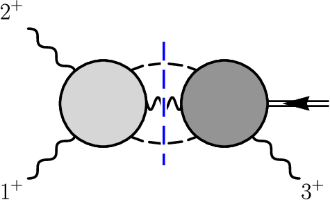
Refer to caption

(a)

Refer to caption

(b)

Figure 8: (a) Unitary cut which determines the renormalization of 𝒪F3\mathcal{O}_{F^{3}} by 𝒪(φ2​F2)1\mathcal{O}_{{(\varphi^{2}F^{2})_{1}}} or 𝒪(φ2​F2)2\mathcal{O}_{{(\varphi^{2}F^{2})_{2}}}. Note this form factor requires q≠0q\neq 0, and the double-lined arrow indicates this insertion of additional off-shell momentum from the operator. (b) Unitarity cut which determines the renormalization of 𝒪(ψ4)1\mathcal{O}_{{(\psi^{4})_{1}}} and 𝒪(ψ4)2\mathcal{O}_{{(\psi^{4})_{2}}} by 𝒪(φ2​F2)1\mathcal{O}_{{(\varphi^{2}F^{2})_{1}}} or 𝒪(φ2​F2)2\mathcal{O}_{{(\varphi^{2}F^{2})_{2}}}. In each, the darker blobs indicate a higher-dimension operator insertion, and the dashed line indicates the integral over phase space of the particles crossing the cut.

4.4 Outlook on additional zeros

F3{{F^{3}}} (φ2​F2)1{{(\varphi^{2}F^{2})_{1}}} (φ2​F2)2{{(\varphi^{2}F^{2})_{2}}} (D2​φ4)1{{(D^{2}\varphi^{4})_{1}}} (D2​φ4)2{{(D^{2}\varphi^{4})_{2}}} (D​φ2​ψ2)1{{(D\varphi^{2}\psi^{2})_{1}}} (D​φ2​ψ2)2{{(D\varphi^{2}\psi^{2})_{2}}} (ψ4)1{{(\psi^{4})_{1}}} (ψ4)2{{(\psi^{4})_{2}}} φ6{{\varphi^{6}}}
F3{{F^{3}}} 0 0 0 0 0 0 0̸\not{0}
(φ2​F2)1{{(\varphi^{2}F^{2})_{1}}} 0 0 0
(φ2​F2)2{{(\varphi^{2}F^{2})_{2}}} 0 0 0
(D2​φ4)1{{(D^{2}\varphi^{4})_{1}}} 0∗ 0∗ 0
(D2​φ4)2{{(D^{2}\varphi^{4})_{2}}} 0∗ 0∗ 0
(D​φ2​ψ2)1{{(D\varphi^{2}\psi^{2})_{1}}} 0̸\not{0}
(D​φ2​ψ2)2{{(D\varphi^{2}\psi^{2})_{2}}} 0̸\not{0}
(ψ4)1{{(\psi^{4})_{1}}} 0 0 0̸\not{0}
(ψ4)2{{(\psi^{4})_{2}}} 0 0 0̸\not{0}
φ6{{\varphi^{6}}}
0̸\not{0} : trivial zero, no contributing two-loop diagrams
0 : zero predicted by the selection rules of Section 4
: only a three-particle cut is needed to evaluate γi​jUV⁡(2)\gamma_{ij}^{\rm UV(2)}
Table 4: Structure of the two-loop anomalous dimension matrix γi​j(2)\gamma_{ij}^{(2)} due to the collected rules outlined in this section. A 0̸\not{0} indicates there are no contributing two-loop diagrams, whereas 00 alone indicates that there are one-loop diagrams that could contribute, but the anomalous dimension evaluates to zero. A 0∗0^{*} indicates the result is nonzero in MS¯\overline{\rm MS}, but set to zero by introducing the appropriate finite counterterms. Shading indicates the entry depends only on the three-particle cut, due to either the length selection rules of Section 4.1 or the vanishing of the relevant one-loop amplitudes. As for Table 2, the operators labeling the rows are renormalized by the operators labeling the columns.

The previous sections have demonstrated numerous zeros in the two-loop anomalous dimension matrix, summarized in Table 4. However, the previous examples are by no means exhaustive, and more zeros may exist. The large number of zeros in the one-loop amplitudes (Table 3) implies that when calculating two-loop anomalous dimensions, the two-particle cut formed from the dimension-four tree and the dimension-six one-loop amplitude will not contribute. In some cases, the only contribution will come from the three-particle cut. Examples of this include the renormalization of 𝒪F3\mathcal{O}_{F^{3}} by 𝒪(φ2​F2)1\mathcal{O}_{{(\varphi^{2}F^{2})_{1}}} or 𝒪(φ2​F2)2\mathcal{O}_{{(\varphi^{2}F^{2})_{2}}}, and the renormalization of 𝒪(ψ4)1\mathcal{O}_{{(\psi^{4})_{1}}} and 𝒪(ψ4)2\mathcal{O}_{{(\psi^{4})_{2}}} by 𝒪(φ2​F2)1\mathcal{O}_{{(\varphi^{2}F^{2})_{1}}} or 𝒪(φ2​F2)2\mathcal{O}_{{(\varphi^{2}F^{2})_{2}}}. The cuts for these examples are depicted in Figure 8. While is may seem that there no reason to expect any given three-particle cut to evaluate to zero, it is possible that a detailed inspection may find that helicity selection rules NonrenormHelicity or angular momentum selection rules Jiang:2020sdh set certain cuts to zero. For a generic entry, the collection of these rules and the rules laid out in the sections above greatly simplify the calculation of the two-loop anomalous dimensions by eliminating one or more required unitary cuts, and one might expect that overlapping rules will conspire to eliminate all possible cuts and set additional entries in Table 4 to zero.

5 Implications for the SMEFT

In this section we describe the overlap of our theory with the SMEFT, and we explain how our calculations directly confirm a large number of the one-loop anomalous dimensions computed in Refs. Manohar123. We also comment on two-loop zeros and the coupling dependence of a subset of the two-loop anomalous-dimension matrix of the SMEFT.

5.1 Mapping our theory to the SMEFT

The full SMEFT is more intricate than the simplified model adopted here, as it includes multiple gauge groups and a number of additional operators. However, by keeping the gauge group to be a general S​U​(N)SU(N), and by leaving the identity of the fermions unspecified, we can access many of the entries of the anomalous-dimension matrix in the full SMEFT basis of operators used by Refs. Manohar123. In particular, since the Higgs transforms under S​U​(2)SU(2), setting N=2N=2 and the number of scalars Ns=1N_{s}=1 allows us to map to anomalous dimensions or four-point amplitudes from representatives of any of the classes of operators in Ref. Manohar123 other than the ψ2​F​φ\psi^{2}F\varphi class (ψ2​X​H\psi^{2}XH in the notation of Ref. Manohar123). Since the scalar is in the fundamental representation that class necessarily involves both a left-handed fermion charged under S​U​(2)SU(2), as well as an uncharged right-handed fermion, which does not fit into our framework. By taking N=3N=3, parts of the anomalous dimensions in the SMEFT containing gluons can also be obtained. In principle, one can also compare anomalous dimensions for additional operators using more sophisticated embeddings of the Standard Model into S​U​(N)SU(N), including U⁡(1)U(1) charges (see e.g, Appendix IV of Ref. ConvertToU1), but we do not do so here.

By specifying the flavor of the fermions, we can map to a number of operators of the full basis used by Ref. Manohar123 via different choices of gauge group and helicity. For example, by taking N=2N=2 and and left-handed helicity on the external states, we access the S​U​(2)SU(2) portions of the amplitudes involving the qq and q¯\overline{q} quark doublets, and map onto the operators (q¯​γμ​q)​(q¯​γμ​q)(\overline{q}\gamma_{\mu}q)(\overline{q}\gamma^{\mu}q) and (q¯​γμ​τI​q)​(q¯​γμ​τI​q)(\overline{q}\gamma_{\mu}\tau^{I}q)(\overline{q}\gamma^{\mu}\tau^{I}q). One remaining difference in our approach compared to the full SMEFT is that we treat the fermions as Dirac instead of Weyl. This causes factor of 2 differences in the NfN_{f} terms of the renormalization of 𝒪(D​φ2​ψ2)2\mathcal{O}_{{(D\varphi^{2}\psi^{2})_{2}}} and 𝒪(ψ4)2\mathcal{O}_{{(\psi^{4})_{2}}} compared to Ref. Manohar123, which need to be taken into account when comparing. While our simplified model avoids having to deal with γ5\gamma_{5}, the generalized unitarity method has been applied to such cases as well ChiralOnShell. At one loop, the issue of Weyl versus Dirac fermions is reduced to a question of which helicities to take in the state sum in Eq. (24).

Setting aside the issue of Weyl versus Dirac fermions, mapping onto the four-fermion operators of Ref. Manohar123, (l¯​γμ​l)​(l¯​γμ​l)(\overline{l}\gamma_{\mu}l)(\overline{l}\gamma^{\mu}l), (u¯​γμ​u)​(u¯​γμ​u)(\overline{u}\gamma_{\mu}u)(\overline{u}\gamma^{\mu}u), and (d¯​γμ​d)​(d¯​γμ​d)(\overline{d}\gamma_{\mu}d)(\overline{d}\gamma^{\mu}d) is possible as well, but requires some care, due to the presence of evanescent effects. In particular, for these cases the operator 𝒪(ψ4)2\mathcal{O}_{{(\psi^{4})_{2}}} is related to the operator 𝒪(ψ4)1\mathcal{O}_{{(\psi^{4})_{1}}} due to the S​U​(N)SU(N) Fierz identity (59)

(ψ¯​γμm​Ta​ψn)​(ψ¯​γμp​Ta​ψr)=(ψ¯​γμm​ψn)​(ψ¯​γμp​ψr)​(δip​in​δim​ir−δim​in​δip​irN).(\overline{\psi}{}_{m}\gamma^{\mu}T^{a}\psi_{n})(\overline{\psi}{}_{p}\gamma_{\mu}T^{a}\psi_{r})=(\overline{\psi}{}_{m}\gamma^{\mu}\psi_{n})(\overline{\psi}{}_{p}\gamma_{\mu}\psi_{r})\left(\delta_{i_{p}i_{n}}\delta_{i_{m}i_{r}}-\frac{\delta_{i_{m}i_{n}}\delta_{i_{p}i_{r}}}{N}\right). (76)

which, together with the Lorentz–Fierz relations for all left- or right-handed spinors

(ψ¯​γμLm​ψLn)​(ψ¯​γμLp​ψLr)\displaystyle(\overline{\psi}{}^{m}_{L}\gamma^{\mu}\psi^{n}_{L})(\overline{\psi}{}^{p}_{L}\gamma_{\mu}\psi^{r}_{L}) =−(ψ¯​γμLp​ψLn)​(ψ¯​γμLm​ψLr),\displaystyle=-(\overline{\psi}{}^{p}_{L}\gamma^{\mu}\psi^{n}_{L})(\overline{\psi}{}^{m}_{L}\gamma_{\mu}\psi^{r}_{L})\,,
(ψ¯​γμRm​ψRn)​(ψ¯​γμRp​ψRr)\displaystyle(\overline{\psi}{}^{m}_{R}\gamma^{\mu}\psi^{n}_{R})(\overline{\psi}{}^{p}_{R}\gamma_{\mu}\psi^{r}_{R}) =−(ψ¯​γμRp​ψRn)​(ψ¯​γμRm​ψRr),\displaystyle=-(\overline{\psi}{}^{p}_{R}\gamma^{\mu}\psi^{n}_{R})(\overline{\psi}{}^{m}_{R}\gamma_{\mu}\psi^{r}_{R})\,, (77)

(where we raised the flavor indices for convenience) can be applied to eliminate the need for the 𝒪(ψ4)2\mathcal{O}_{{(\psi^{4})_{2}}} operator in Table 1:

𝒪(ψ4)2m​n​p​r=(ψ¯​γμm​Ta​ψn)​(ψ¯​γμp​Ta​ψr)=𝒪(ψ4)1m​r​p​n−1N​𝒪(ψ4)1m​n​p​r,\displaystyle\mathcal{O}_{{(\psi^{4})_{2}}}^{mnpr}=(\overline{\psi}{}_{m}\gamma^{\mu}T^{a}\psi_{n})(\overline{\psi}{}_{p}\gamma_{\mu}T^{a}\psi_{r})=\mathcal{O}_{{(\psi^{4})_{1}}}^{mrpn}-\frac{1}{N}\mathcal{O}_{{(\psi^{4})_{1}}}^{mnpr}\,, (78)

when there are no additional group indices preventing the particle exchange (for example, the additional S​U​(3)SU(3) index prevents the reduction of (q¯​γμ​τI​q)​(q¯​γμ​τI​q)(\overline{q}\gamma^{\mu}\tau^{I}q)(\overline{q}\gamma_{\mu}\tau^{I}q) operator based on the S​U​(2)SU(2) Fierz identity). By choosing to implement Eq. (77) or not, we can map onto either the operators (l¯​γμ​l)​(l¯​γμ​l)(\overline{l}\gamma^{\mu}l)(\overline{l}\gamma_{\mu}l), (u¯​γμ​u)​(u¯​γμ​u)(\overline{u}\gamma^{\mu}u)(\overline{u}\gamma_{\mu}u), or (d¯​γμ​d)​(d¯​γμ​d)(\overline{d}\gamma^{\mu}d)(\overline{d}\gamma_{\mu}d), or onto the set of operators (q¯​γμ​τI​q)​(q¯​γμ​τI​q)(\overline{q}\gamma^{\mu}\tau^{I}q)(\overline{q}\gamma_{\mu}\tau^{I}q) and (q¯​γμ​τI​q)​(q¯​γμ​τI​q)(\overline{q}\gamma^{\mu}\tau^{I}q)(\overline{q}\gamma_{\mu}\tau^{I}q), respectively. Since we take all the fermions in our operators to be charged under the same gauge group, here we do not map onto the (L¯​R)​(L¯​R)(\overline{L}R)(\overline{L}R) or (L¯​R)​(R¯​L)(\overline{L}R)(\overline{R}L) subsets of the four-fermion operators, which require the presence of multiple gauge groups.

It is worth noting, that there are some simplifications in the SMEFT relative to our model with general gauge group. The symmetric color tensor da​b​cd^{abc} is zero in S​U​(2)SU(2), meaning that the operator 𝒪(φ2​F2)2\mathcal{O}_{{(\varphi^{2}F^{2})_{2}}} is identically zero. In addition, this implies the color factors for the two-vector, two-scalar or two-vector, two-fermion processes are related by N​{Ta1,Ta2}i4​i3=2​δa1​a2​δi4​i3N\{T^{a_{1}},T^{a_{2}}\}_{i_{4}i_{3}}=2\delta^{a_{1}a_{2}}\delta_{i_{4}i_{3}}, meaning the number of color-ordered amplitudes is reduced for those processes in the case of S​U​(2)SU(2).

𝒪G\mathcal{O}_{G} 𝒪W\mathcal{O}_{W} 𝒪H​W\mathcal{O}_{HW}
𝒪H​□\mathcal{O}_{H\Box}
𝒪H​D\mathcal{O}_{HD}
𝒪H​l(1)\mathcal{O}_{Hl}^{(1)}
𝒪H​l(3)\mathcal{O}_{Hl}^{(3)}
𝒪H​q(1)\mathcal{O}_{Hq}^{(1)}
𝒪H​q(3)\mathcal{O}_{Hq}^{(3)}
𝒪l​l\mathcal{O}_{ll}
𝒪q​q(1)\mathcal{O}_{qq}^{(1)}
𝒪q​q(3)\mathcal{O}_{qq}^{(3)}
𝒪u​u\mathcal{O}_{uu}
𝒪d​d\mathcal{O}_{dd}
𝒪G\mathcal{O}_{G} ✓3{\color[rgb]{0,0,1}\checkmark_{3}} 0̸\not{0} 0̸\not{0} 0̸\not{0} 0̸\not{0} 0̸\not{0} 0̸\not{0} 0̸\not{0} 0̸\not{0}
𝒪W\mathcal{O}_{W} 0̸\not{0} ✓2{\color[rgb]{0,0,1}\checkmark_{2}} ✓2{\color[rgb]{0,0,1}\checkmark_{2}} 0̸\not{0} 0̸\not{0} 0̸\not{0} 0̸\not{0} 0̸\not{0} 0̸\not{0}
𝒪H​W\mathcal{O}_{HW} 0̸\not{0} ✓2{\color[rgb]{0,0,1}\checkmark_{2}} ✓2,λ{\color[rgb]{0,0,1}\checkmark_{2,\lambda}} ✓2{\color[rgb]{0,0,1}\checkmark_{2}} ✓2{\color[rgb]{0,0,1}\checkmark_{2}} ✓2{\color[rgb]{0,0,1}\checkmark_{2}} 0̸\not{0} 0̸\not{0} 0̸\not{0}
𝒪H​□,𝒪H​D\mathcal{O}_{H\Box},\,\mathcal{O}_{HD} 0̸\not{0} ✓2{\color[rgb]{0,0,1}\checkmark_{2}} ✓2{\color[rgb]{0,0,1}\checkmark_{2}} ✓2,λ{\color[rgb]{0,0,1}\checkmark_{2,\lambda}} ✓2{\color[rgb]{0,0,1}\checkmark_{2}} ✓2{\color[rgb]{0,0,1}\checkmark_{2}} 0̸\not{0} 0̸\not{0} 0̸\not{0}
𝒪H​l(1),𝒪H​l(3)\mathcal{O}_{Hl}^{(1)},\,\mathcal{O}_{Hl}^{(3)} 0̸\not{0} ✓2{\color[rgb]{0,0,1}\checkmark_{2}} ✓2{\color[rgb]{0,0,1}\checkmark_{2}} ✓2{\color[rgb]{0,0,1}\checkmark_{2}} ✓2,λ{\color[rgb]{0,0,1}\checkmark_{2,\lambda}} ✓2{\color[rgb]{0,0,1}\checkmark_{2}} ✓2{\color[rgb]{0,0,1}\checkmark_{2}} 0̸\not{0} 0̸\not{0}
𝒪H​q(1),𝒪H​q(3)\mathcal{O}_{Hq}^{(1)},\,\mathcal{O}_{Hq}^{(3)} 0̸\not{0} ✓2{\color[rgb]{0,0,1}\checkmark_{2}} ✓2{\color[rgb]{0,0,1}\checkmark_{2}} ✓2{\color[rgb]{0,0,1}\checkmark_{2}} ✓2{\color[rgb]{0,0,1}\checkmark_{2}} ✓2,λ{\color[rgb]{0,0,1}\checkmark_{2,\lambda}} 0̸\not{0} ✓2{\color[rgb]{0,0,1}\checkmark_{2}} 0̸\not{0}
𝒪l​l\mathcal{O}_{ll} 0̸\not{0} ✓2{\color[rgb]{0,0,1}\checkmark_{2}} 0̸\not{0} 0̸\not{0} ✓2{\color[rgb]{0,0,1}\checkmark_{2}} 0̸\not{0} ✓2{\color[rgb]{0,0,1}\checkmark_{2}} 0̸\not{0} 0̸\not{0}
𝒪q​q(1),𝒪q​q(3)\mathcal{O}_{qq}^{(1)},\,\mathcal{O}_{qq}^{(3)} ✓3{\color[rgb]{0,0,1}\checkmark_{3}} ✓2{\color[rgb]{0,0,1}\checkmark_{2}} 0̸\not{0} 0̸\not{0} 0̸\not{0} ✓2{\color[rgb]{0,0,1}\checkmark_{2}} 0̸\not{0} ✓2{\color[rgb]{0,0,1}\checkmark_{2}} 0̸\not{0}
𝒪u​u,𝒪d​d\mathcal{O}_{uu},\,\mathcal{O}_{dd} ✓3{\color[rgb]{0,0,1}\checkmark_{3}} 0̸\not{0} 0̸\not{0} 0̸\not{0} 0̸\not{0} 0̸\not{0} 0̸\not{0} 0̸\not{0} ✓3{\color[rgb]{0,0,1}\checkmark_{3}}
Table 5: Checks on the one-loop anomalous dimensions calculated in Ref. Manohar123 obtained from our calculations. The 0̸\not{0} entries correspond to trivial cases were there are no contributing diagrams. The entries ✓3\checkmark_{3} and ✓2\checkmark_{2} are checked by setting the SU(N) group to SU(3) or SU(2), respectively. In both cases, only the pieces of the anomalous dimensions proportional to g32g_{3}^{2} or g22g_{2}^{2} are accessed by our amplitudes. The ✓2,λ\checkmark_{2,\lambda} cases indicates that both terms proportional to g22g_{2}^{2} and λ\lambda are verified. Operators have been grouped according to whether the gauge dependence of the particle content is the same. As for the other tables, the operators labeling the rows are renormalized by the operators labeling the columns.

5.2 Verification of one-loop anomalous dimensions

From our one-loop calculations and the relations described above we have verified entries from numerous classes of operators in the SMEFT, as summarized in Table 5, following the notation of Ref. Manohar123. This includes examples proportional to g32g_{3}^{2}, g22g_{2}^{2}, and λ\lambda. In this sense our operators are a representative sample of the full SMEFT, despite the simplified nature of our dimension-four Lagrangian. The direct agreement with results of Ref. Manohar123 displayed in Table 5 provides a highly non-trivial check of the validity and the effectiveness of the approach used here.

5.3 Two-loop implications

𝒪G\mathcal{O}_{G} 𝒪W\mathcal{O}_{W} 𝒪H​W\mathcal{O}_{HW} 𝒪u​W\mathcal{O}_{uW}
𝒪H​□\mathcal{O}_{H\Box}
𝒪H​D\mathcal{O}_{HD}
𝒪H​q(1)\mathcal{O}_{Hq}^{(1)}
𝒪H​q(3)\mathcal{O}_{Hq}^{(3)}
𝒪q​q(1)\mathcal{O}_{qq}^{(1)}
𝒪q​q(3)\mathcal{O}_{qq}^{(3)}
𝒪u​u\mathcal{O}_{uu} 𝒪u​H\mathcal{O}_{uH} 𝒪H\mathcal{O}_{H}
𝒪G\mathcal{O}_{G} 0̸\not{0} 0̸\not{0} 0̸\not{0} 0̸\not{0} 0̸\not{0} 0 0 0̸\not{0} 0̸\not{0}
𝒪W\mathcal{O}_{W} 0̸\not{0} 0y0_{y} 0 0 0 0̸\not{0} 0̸\not{0} 0̸\not{0}
𝒪H​W\mathcal{O}_{HW} 0̸\not{0} 0y0_{y} 00 0̸\not{0} 0y0_{y} 0
𝒪u​W\mathcal{O}_{uW} 0y0_{y} 0y0_{y} 0y0_{y} 0y0_{y} 0y0_{y} 0y0_{y} 0y0_{y} 0̸\not{0}
𝒪H​□,𝒪H​D\mathcal{O}_{H\Box},\,\mathcal{O}_{HD} 0̸\not{0} 0y0_{y} 0y​(g24∗)0_{y}(\bcancel{g_{2}^{4}}^{*}) 0y0_{y} 0y0_{y} 0
𝒪H​q(1),𝒪H​q(3)\mathcal{O}_{Hq}^{(1)},\,\mathcal{O}_{Hq}^{(3)} 0y0_{y} 0y0_{y} 0y​(y​λ)0_{y}(\bcancel{y\lambda}) 0̸\not{0}
𝒪q​q(1),𝒪q​q(3)\mathcal{O}_{qq}^{(1)},\,\mathcal{O}_{qq}^{(3)} 0y0_{y} 0y​(g24)0_{y}(\bcancel{g_{2}^{4}}) 0̸\not{0} 0̸\not{0}
𝒪u​u\mathcal{O}_{uu} 0̸\not{0} 0̸\not{0} 0y0_{y} 0y0_{y} 0y0_{y} 0̸\not{0} 0̸\not{0}
𝒪u​H\mathcal{O}_{uH} 0y0_{y} 0y0_{y} 0y0_{y} 0y0_{y} 0y0_{y} 0y0_{y} 0y0_{y} 0y0_{y}
𝒪H\mathcal{O}_{H} 0̸\not{0} 0y0_{y} 0y0_{y}
0̸\not{0} : trivial zero, no contributing two-loop diagrams
0 : zero predicted by the selection rules of Section 4
: only a three-particle cut is needed to evaluate γi​jUV⁡(2)\gamma_{ij}^{\rm UV(2)}
: only two-particle cuts available for the relevant diagrams
0​(y​λ)0(\bcancel{y\lambda}), etc. : the selection rules of Section 4 forbid the stated coupling dependence
0y0_{y} : γi​jUV⁡(2)\gamma_{ij}^{\rm UV(2)} vanishes if Yukawa couplings are set to zero
Table 6: Predictions for the zeros and coupling dependences of a representative selection of the SMEFT two-loop anomalous-dimension matrix, γi​jUV⁡(2)\gamma_{ij}^{\rm UV(2)}. The notation for the operator labels follows that of Manohar123. The g24g_{2}^{4} dependence of the entry labeled 0y​(g24∗)0_{y}(\bcancel{g_{2}^{4}}^{*}) vanishes using the appropriate counterterms at one loop. The operators labeling the rows are renormalized by the operators labeling the columns.

Next we briefly discuss the implications of the zeros in the two-loop anomalous dimensions of our simplifies model for the SMEFT. The selection rules of Section 4 set a number of entries strictly to zero, and restrict the coupling dependence of others. Our findings are summarized in Table 6. The full SMEFT anomalous dimensions include dependence on the Yukawa couplings, which are absent in our simplified theory, so some of the zeros uncovered above may be replaced by anomalous dimensions that depend on such couplings. Nevertheless, our results show that the coupling dependence of the anomalous dimensions is simpler than one might have expected, and that some of the entries are zero or do not have pure dependence on the gauge couplings. Though most of the strictly zero examples rely on the length selection rule, which does not depend on the gauge group or the presence of Yukawa couplings, the anomalous-dimension matrix element γH​W←q​q(2)\gamma_{HW\leftarrow qq}^{(2)} relies solely on the color selection rules. In this case, including Yukawa and U(1) couplings will not affect this zero, as the cuts still cannot match the color of the target operator.

In addition to the zeros, we find that many of the entries only receive contributions from either three- or two-particle cuts, which should greatly simplify their computation. One interesting example is the element γq​q←H​W(2)\gamma_{qq\leftarrow HW}^{(2)}, which only has a three-particle cut due to the vanishing of the one-loop amplitudes that would contribute to the two-particle cut. For this example, we have also checked the one-loop amplitudes with Yukawa and U(1) couplings do not contribute. As can also be seen in Table 6, many entries vanish when the Yukawa couplings are set to zero. Many of these zeros are trivial due to the particle content of the operators involved, but in some cases a closer examination of the diagrams is required to see that only diagrams with Yukawa couplings will produce nonvanishing results.

Note that the operators in Table 6 are merely a representative set, in that all of the operators of the SMEFT are restricted by one or more of our selection rules, either in terms of which operators they can renormalize, or vice versa. In particular, the length selection rules apply independently of the gauge group or the presence of Yukawa couplings, which allows us to include operators of the classes ψ2​F​φ\psi^{2}F\varphi and ψ2​φ3\psi^{2}\varphi^{3} in Table 6. We would also like to stress that our analysis of the structure of the two-loop anomalous dimensions is not an exhaustive study of the SMEFT anomalous dimensions. For this reason, we expect that there could be additional vanishings or structures that can be uncovered under closer scrutiny.

6 Conclusions

In this paper we applied on-shell methods to investigate the structure of the two-loop anomalous dimension matrix of dimension-six operators, in both a simplified model and in the SMEFT. At one loop, we used both the standard generalized unitarity method GeneralizedUnitarity1 and the recently developed approach for extracting anomalous dimensions directly from unitarity cuts Caron-Huot:2016cwu. At two loops, we find the latter method to be especially effective, with the former method providing one-loop amplitudes as inputs. As an initial step, we reorganized the basic equation for the two-loop anomalous dimension in the latter approach so as to simplify one-loop iterations. Using this equation, we revealed a number of vanishing contributions in the two-loop anomalous dimension matrix of the SMEFT. Our analysis was based on a simplified model without U(1) or Yukawa interactions. Nevertheless, as summarized in Table 6, by analyzing the overlap of our simplified model with the SMEFT we found that a remarkable number of SMEFT two-loop anomalous dimensions either vanish or have a simpler dependence on the Standard Model couplings than naively expected.

The structure we uncovered has a number of origins, including length selection rules, color selection rules, and zeros in the one-loop amplitudes with dimension-six operator insertions. Additional zeros arise from the choice of an MS¯\overline{\rm MS}-like scheme which includes additional finite renormalizations designed to set various rational terms in one-loop amplitudes to zero. This suggests that there exist interesting schemes that make the structure of the renormalization-group running beyond one loop more transparent. The full implications of choosing such schemes clearly deserve further study.

Since one-loop amplitudes are used as input for the two-loop calculation, we have computed the full set of four-point amplitudes with dimension-six operator insertions in our simplified version of the SMEFT. As a byproduct, these amplitudes have allowed us to verify a large subset of the one-loop anomalous dimensions calculated in Refs. Manohar123.

The zeros that we found in the two-loop anomalous dimension matrix relied on choosing examples with trivial infrared dependence, as well as a lack of a three-particle cut. However, the methods can be applied just as well to any generic anomalous dimension matrix element at two or higher loops. It would be interesting to investigate whether there are additional zeros at two loops beyond those we identified. The large number of zeros in the one-loop amplitudes restrict the number of cuts that can contribute, suggesting that other mechanisms, such as helicity or angular-momentum selection rules, may set the remaining cuts to zero in some cases.

The presented methods are quite general, and should be applicable to general EFTs. In addition, while we have focused on ultraviolet anomalous dimensions here, this method could equally be applied to the evaluation of infrared anomalous dimensions, such as the soft anomalous dimension, by the use of ultraviolet protected operators such as the stress-tensor or global symmetry currents. It would also be interesting to understand the implications, if any, of the vanishing of two-loop anomalous dimensions for the interference of Standard Model and higher-dimension operator matrix elements beyond tree level, in the presence of experimental cuts. Another obvious direction would be to include dimension seven and eight operators into the analysis Dim78.

In summary, we have demonstrated that the on-shell methods applied here are well suited for computing anomalous dimensions and associated scattering amplitudes at one and two loops. We used these methods to expose new structures in the guise of vanishing terms in the anomalous matrix of the SMEFT beyond one loop. Our analysis here was not exhaustive, so it is likely that further vanishing contributions and new structures exist at two loops and beyond. Our results also suggest that a judicious choice of renormalization scheme can help expose such structures.

Acknowledgments

We thank Clifford Cheung, Nathaniel Craig, Enrico Herrmann, Chia-Hsien Shen and especially Aneesh Manohar for many helpful discussions. Z.B. is supported by the U.S. Department of Energy (DOE) under award number DE-SC0009937. J.P-.M. is supported by the US Department of State through a Fulbright scholarship. We are also grateful to the Mani L. Bhaumik Institute for Theoretical Physics for additional support.

Appendix A Integral reduction via gauge-invariant tensors

In this appendix we summarize the projection technique that we use to perform tensor reduction of loop integrals in Section 3. The same technique has been previously used in Refs. Projectors1; Projectors2 and is a convenient method for decomposing DD-dimensional tensor loop integrands (or cuts) into a basis of scalar master integrals, in a way that makes dimensional regularization, and any associated chiral and evanescent issues relatively straightforward. In particular this technique is well suited to deal with integrals with high-rank numerators, which naturally arise in loop amplitudes with insertions of higher-dimension operators.

We start by noting that scattering amplitudes amplitudes are gauge invariant and can therefore be decomposed into a basis of gauge-invariant tensors, TmT_{m}. For a given amplitude labeled by ii we have,

Ai(L)=∑m𝒜i,m(L)​(kj)​Tm​(kj,ϵj,uj,u¯j),A^{(L)}_{i}=\sum_{m}\mathcal{A}^{(L)}_{i,m}(k_{j})T_{m}(k_{j},\epsilon_{j},u_{j},\overline{u}_{j})\,, (79)

where the coefficients, 𝒜i,m(L)\mathcal{A}^{(L)}_{i,m}, only depend on the external momenta, and all dependence on the polarization vectors or spinors is contained entirely within the basis tensors, TmT_{m}. The basis tensors for the various processes we consider in this paper are given below and in the supplementary material AttachedFiles. They are found by writing down the most general polynomials built from Lorentz invariant products of external polarizations, spinor and momenta and then demanding gauge invariance.

The desired coefficient of tensor TjT_{j} can be extracted using a projector

Pn=cn​m​Tm∗,P_{n}=c_{nm}T_{m}^{*}\,, (80)

where cn​mc_{nm} is the inverse of the matrix

mn​m=Tn∗⊙Tm.m_{nm}=T^{*}_{n}\odot T_{m}\,. (81)

Here the product ⊙\odot corresponds to the state sum in Eq. (41), taken over all particles. The coefficient of the tensor is then simply given by

𝒜i,m(L)=Pm⊙Ai(L).\mathcal{A}^{(L)}_{i,m}=P_{m}\odot A^{(L)}_{i}\,. (82)

The projectors for all processes consider in this paper are given explicitly in an ancillary file AttachedFiles.

Once projected, any gauge invariant quantity can be summarized as a list of the coefficients corresponding to each basis tensor. In the case of a loop integrand or cut thereof, each coefficient is a rational function of scalar propagators and inverse propagators (and irreducible numerators beyond one loop). The integrals corresponding to each term in the projected quantity are then in a form that can be reduced to a basis of master integrals using by integration by parts (IBP) relations. This can be done using by using IBP programs such as FIRE FIRE.

As described in Section 3, we can apply this procedure cut by cut to determine the coefficients of each gauge invariant tensor in the full amplitude.

Basis tensors

Basis tensors for the four-vector amplitudes are taken from Projectors2, which we reproduce here. Beginning with the linearized field strength for each external particle:

Fi​μ​ν≡ki​μ​εi​ν−ki​ν​εi​μ,F_{i\,\mu\nu}\equiv k_{i\,\mu}\varepsilon_{i\,\nu}-k_{i\,\nu}\varepsilon_{i\,\mu}\,, (83)

one can construct the following combinations,

Fs​t4\displaystyle F^{4}_{st} ≡(F1​F2​F3​F4),\displaystyle\equiv(F_{1}F_{2}F_{3}F_{4})\,, Ft​u4\displaystyle F^{4}_{tu} ≡(F1​F4​F2​F3),\displaystyle\equiv(F_{1}F_{4}F_{2}F_{3})\,, Fu​s4\displaystyle F^{4}_{us} ≡(F1​F3​F4​F2),\displaystyle\equiv(F_{1}F_{3}F_{4}F_{2})\,, (84)
(Fs2)2\displaystyle(F^{2}_{s})^{2} ≡(F1F2)(F3F4),\displaystyle\equiv(F_{1}F_{2})(F_{3}F_{4})\,,\hskip 14.22636pt (Ft2)2\displaystyle(F^{2}_{t})^{2} ≡(F1F4)(F2F3),\displaystyle\equiv(F_{1}F_{4})(F_{2}F_{3})\,,\hskip 14.22636pt (Fu2)2\displaystyle(F^{2}_{u})^{2} ≡(F1​F3)​(F4​F2),\displaystyle\equiv(F_{1}F_{3})(F_{4}F_{2})\,,

where parentheses one the right-hand side of the above equations indicate taking the trace over adjacent Lorentz indices. The four-vector basis tensors are then given by

Tv​v​v​vtree\displaystyle T_{vvvv}^{\rm tree} =−12​((Fs2)2+(Ft2)2+(Fu2)2)+2​(Fs​t4+Ft​u4+Fu​s4),\displaystyle=-\frac{1}{2}((F^{2}_{s})^{2}+(F^{2}_{t})^{2}+(F^{2}_{u})^{2})+2\,(F^{4}_{st}+F^{4}_{tu}+F^{4}_{us})\,,
Tv​v​v​v++++\displaystyle T_{vvvv}^{++++} =−2​Fs​t4+12​((Fs2)2+(Ft2)2+(Fu2)2),\displaystyle=-2\,F^{4}_{st}+\frac{1}{2}\,((F^{2}_{s})^{2}+(F^{2}_{t})^{2}+(F^{2}_{u})^{2})\,,
Tv​v​v​v−+++\displaystyle T_{vvvv}^{-+++} =−TF3−(Ft​u4−Fu​s4)​(s−t)+(Fs​t4−14​((Fs2)2+(Ft2)2+(Fu2)2))​(s+t),\displaystyle=-T_{F^{3}}-(F^{4}_{tu}-F^{4}_{us})\,(s-t)+(F^{4}_{st}-\frac{1}{4}((F^{2}_{s})^{2}+(F^{2}_{t})^{2}+(F^{2}_{u})^{2}))\,(s+t)\,,
Tv​v​v​v−−++\displaystyle T_{vvvv}^{--++} =(Fs2)2−(Ft2)2+2​(Ft​u4−Fu​s4),\displaystyle=(F^{2}_{s})^{2}-(F^{2}_{t})^{2}+2\,(F^{4}_{tu}-F^{4}_{us})\,, (85)
Tv​v​v​v−+−+\displaystyle T_{vvvv}^{-+-+} =2​Fs​t4−12​((Fs2)2+(Ft2)2−(Fu2)2),\displaystyle=2\,F^{4}_{st}-\frac{1}{2}((F^{2}_{s})^{2}+(F^{2}_{t})^{2}-(F^{2}_{u})^{2})\,,
Tv​v​v​vev1\displaystyle T_{vvvv}^{\rm ev1} =−(2​Fs​t4+32​((Fs2)2+(Ft2)2+(Fu2)2))​(s+t)+2​(Fu​s4​(3​s+t)+Ft​u4​(s+3​t)),\displaystyle=-(2\,F^{4}_{st}+\frac{3}{2}\,((F^{2}_{s})^{2}+(F^{2}_{t})^{2}+(F^{2}_{u})^{2}))\,(s+t)+2\,(F^{4}_{us}\,(3\,s+t)+F^{4}_{tu}\,(s+3\,t))\,,
Tv​v​v​vev2\displaystyle T_{vvvv}^{\rm ev2} =−(2​Fs​t4−12​((Fs2)2+(Ft2)2+(Fu2)2))​(s−t)+2​(Ft​u4−Fu​s4)​(s+t),\displaystyle=-(2\,F^{4}_{st}-\frac{1}{2}((F^{2}_{s})^{2}+(F^{2}_{t})^{2}+(F^{2}_{u})^{2}))\,(s-t)+2\,(F^{4}_{tu}-F^{4}_{us})\,(s+t)\,,

where the vv labels signifies that a leg is a vector boson, and TF3T_{F^{3}} is proportional to the F3F^{3} amplitude SupersymStringAmps:

TF3=−i​s​t​AF3(0)=−i​s​t​u​((Fs2)24​s2+(Ft2)24​t2+(Fu2)24​u2−g1​g2​g3​g4(s​t​u)2),T_{F^{3}}=-istA_{F^{3}}^{(0)}=-istu\left(\frac{(F_{s}^{2})^{2}}{4s^{2}}+\frac{(F_{t}^{2})^{2}}{4t^{2}}+\frac{(F_{u}^{2})^{2}}{4u^{2}}-\frac{g_{1}g_{2}g_{3}g_{4}}{(stu)^{2}}\right)\,, (86)

where gi≡(ki+1​Fi​ki−1)g_{i}\equiv(k_{i+1}F_{i}k_{i-1}). We note that we have written this expression in an explicitly gauge-invariant form at the expense of manifest locality. These tensors are nonzero only under the indicated (and parity conjugate) helicity configurations, along with cyclic permutations. Tv​v​v​vtreeT_{vvvv}^{\rm tree} is nonzero for helicities (1−​2+​3−​4+)(1^{-}2^{+}3^{-}4^{+}), (1−​2−​3+​4+)(1^{-}2^{-}3^{+}4^{+}), and cyclic permutations. Tv​v​v​vev1T_{vvvv}^{\rm ev1} and Tv​v​v​vev2T_{vvvv}^{\rm ev2} are evanescent, i.e. zero for all helicity configurations in four dimensions. This can be made manifest by rewriting them as

Tv​v​v​vev1=12k4[αF1μ​νF2σρ]k2αF4μ​νF3σ​ρ+12k4[αF3μ​νF2σρ]k2αF4μ​νF1σ​ρ,Tv​v​v​vev2=12k2[αF1μ​νF3σρ]k1αF2μ​νF4σ​ρ,\displaystyle\begin{split}T_{vvvv}^{\rm ev1}&=\frac{1}{2}k_{4}^{[\alpha}F_{1}^{\vphantom{[}\mu\nu}F_{2}^{\sigma\rho]}k_{2}{}_{\alpha}F_{4}{}_{\mu\nu}F_{3}{}_{\sigma\rho}+\frac{1}{2}k_{4}^{[\alpha}F_{3}^{\vphantom{[}\mu\nu}F_{2}^{\sigma\rho]}k_{2}{}_{\alpha}F_{4}{}_{\mu\nu}F_{1}{}_{\sigma\rho}\,,\\ T_{vvvv}^{\rm ev2}&=\frac{1}{2}k_{2}^{[\alpha}F_{1}^{\vphantom{[}\mu\nu}F_{3}^{\sigma\rho]}k_{1}{}_{\alpha}F_{2}{}_{\mu\nu}F_{4}{}_{\sigma\rho}\,,\end{split} (87)

where the anti-symmetrization does not include a symmetry factor.

The two-vector, two-scalar tensors are also nonzero under specific helicity combinations, and are given by

Tv​v​s​s+⁣−\displaystyle T^{+-}_{vvss} =2​(k3​F1​F2​k4)+2​(k4​F1​F2​k3)−(k3⋅k4)​(F1​F2),Tv​v​s​s+⁣+\displaystyle=2(k_{3}F_{1}F_{2}k_{4})+2(k_{4}F_{1}F_{2}k_{3})-(k_{3}\cdot k_{4})(F_{1}F_{2})\,,\quad T^{++}_{vvss} =−(F1​F2),\displaystyle=-(F_{1}F_{2})\,, (88)

where the vv and ss labels specify the corresponding legs are vectors or scalars.

Similarly, the two-vector, two-fermion tensors are linear combinations of those in Ref. Projectors1, chosen to again be nonzero only under specific helicities:

Tf​f​v​v−+++=−124(u¯2F̸4F̸3k̸2u1),Tf​f​v​v−+−+=−124(u¯2F̸4k̸2F̸3u1),\displaystyle T^{-+++}_{ffvv}=-\frac{1}{2^{4}}(\overline{u}_{2}\not{F}_{4}\not{F}_{3}\not{k}_{2}u_{1})\,,\qquad T^{-+-+}_{ffvv}=-\frac{1}{2^{4}}(\overline{u}_{2}\not{F}_{4}\not{k}_{2}\not{F}_{3}u_{1})\,,
Tf​f​v​v−++−=−124(u¯2F̸3k̸1F̸4u1),Tf​f​v​v−+−−=−124(u¯2k̸1F̸4F̸3u1),\displaystyle T^{-++-}_{ffvv}=-\frac{1}{2^{4}}(\overline{u}_{2}\not{F}_{3}\not{k}_{1}\not{F}_{4}u_{1})\,,\qquad T^{-+--}_{ffvv}=-\frac{1}{2^{4}}(\overline{u}_{2}\not{k}_{1}\not{F}_{4}\not{F}_{3}u_{1})\,,
Tf​f​v​vev=12k1[αF3μ​νF4ρσ](u¯2γαγμγνγργσu1),\displaystyle\hskip 56.9055ptT^{\rm ev}_{ffvv}=\frac{1}{2}k_{1}^{[\alpha}F_{3}^{\mu\nu}F_{4}^{\rho\sigma]}(\overline{u}_{2}\gamma_{\alpha}\gamma_{\mu}\gamma_{\nu}\gamma_{\rho}\gamma_{\sigma}u_{1})\,, (89)

where ff now indicates a leg as a fermion, F̸i=Fi​μ​ν​γμ​γν\not{F}_{i}=F_{i\,\mu\nu}\gamma^{\mu}\gamma^{\nu}, and the antisymmetrization in TevT^{\rm ev} includes a symmetry factor of 1/5!1/5!. As for the four-vector case, we encounter an evanescent tensor, Tf​f​v​vevT^{\rm ev}_{ffvv} which vanishes for all four-dimensional helicities. For the two-fermion two-scalar case there is only a single basis tensor:

Tf​f​s​s=u¯2​k̸3​u1.\displaystyle T_{ffss}=\overline{u}_{2}\not{k}_{3}u_{1}\,. (90)

Finally, the four-fermion tensors are,

Tf​f​f​f1\displaystyle T^{1}_{ffff} =(u¯2​γμ​u1)​(u¯4​γμ​u3),\displaystyle=(\overline{u}_{2}\gamma^{\mu}u_{1})(\overline{u}_{4}\gamma_{\mu}u_{3})\,,
Tf​f​f​f2\displaystyle T^{2}_{ffff} =(u¯2​k̸4​u1)​(u¯4​k̸2​u3),\displaystyle=(\overline{u}_{2}\not{k}_{4}u_{1})(\overline{u}_{4}\not{k}_{2}u_{3})\,,
Tf​f​f​f3\displaystyle T^{3}_{ffff} =(u¯2​γμ​γν​γρ​u1)​(u¯4​γμ​γν​γρ​u3)−16​(u¯2​γμ​u1)​(u¯4​γμ​u3),\displaystyle=(\overline{u}_{2}\gamma^{\mu}\gamma^{\nu}\gamma^{\rho}u_{1})(\overline{u}_{4}\gamma_{\mu}\gamma_{\nu}\gamma_{\rho}u_{3})-16(\overline{u}_{2}\gamma^{\mu}u_{1})(\overline{u}_{4}\gamma_{\mu}u_{3})\,,
Tf​f​f​f4\displaystyle T^{4}_{ffff} =t⁡(u¯2​γμ​k̸4​γρ​u1)​(u¯4​γμ​k̸2​γρ​u3)−4​u​(u¯2​k̸4​u1)​(u¯4​k̸2​u3),\displaystyle=t\,(\overline{u}_{2}\gamma^{\mu}\not{k}_{4}\gamma^{\rho}u_{1})(\overline{u}_{4}\gamma_{\mu}\not{k}_{2}\gamma_{\rho}u_{3})-4u(\overline{u}_{2}\not{k}_{4}u_{1})(\overline{u}_{4}\not{k}_{2}u_{3})\,, (91)

plus those given by the exchange of legs 2 and 4. It should be noted, however, that in practice it is unnecessary to calculate the coefficients of the exchanged tensors, since they are fixed by the symmetry of the contributing diagrams. Tf​f​f​f3T^{3}_{ffff} and Tf​f​f​f4T^{4}_{ffff} are chosen to be zero for the helicity configuration 1ψ+2ψ¯− 3ψ+4ψ¯−{1{}_{\vphantom{\overline{\psi}}\psi}^{+}}{2{}_{\,\overline{\psi}}^{-}\,}{3{}_{\vphantom{\overline{\psi}}\psi}^{+}}{4{}_{\,\overline{\psi}}^{-}\,} and its conjugate, so that these tensors are evanescent if the spinors are Weyl of the same handedness.

Appendix B Tree-level and one-loop amplitudes

In this appendix we collect tree- and one-loop amplitudes. In addition to the spinor-helicity amplitudes given below, expressions that are valid to all orders in the dimensional regularization parameter ϵ\epsilon are provided in a supplementary file AttachedFiles. While we do not require one-loop amplitudes without higher-dimension operators for our specific examples in Section 4, they would be required for the calculation of a generic two-loop anomalous dimension matrix element. These one-loop dimension-4 amplitudes can be found in various references; e.g. Refs. OneLoopSMAmplitudes gives the relevant amplitudes which exclude scalars.

The amplitudes and form factors can be written as vectors in color space,

A(L)​(λ1​λ2​λ3​λ4)=Sλ1​λ2​λ3​λ4​∑i𝒞λ1​λ2​λ3​λ4[i]​A(L)​(λ1​λ2​λ3​λ4)[i],A^{(L)}(\lambda_{1}\lambda_{2}\lambda_{3}\lambda_{4})=S_{\lambda_{1}\lambda_{2}\lambda_{3}\lambda_{4}}\sum_{i}\mathcal{C}_{\lambda_{1}\lambda_{2}\lambda_{3}\lambda_{4}}^{[i]}A^{(L)}(\lambda_{1}\lambda_{2}\lambda_{3}\lambda_{4})_{[i]}\,, (92)

where Sλ1​λ2​λ3​λ4S_{\lambda_{1}\lambda_{2}\lambda_{3}\lambda_{4}} is a helicity-dependent factor which which depending on spinors when evaluated using four-dimensional spinor helicity. These factors are pure phases for the amplitudes with an even number of pairs of external fermions, and for the amplitudes with an odd number of fermions their square is a dimensionless ratio of s,ts,t, or uu and powers thereof. The full list of Sλ1​λ2​λ3​λ4S_{\lambda_{1}\lambda_{2}\lambda_{3}\lambda_{4}} for each process is listed below.

The IR dependence has been stripped from the amplitudes below, but can be reconstructed, if desired, using the basic IR formulas given in the text, which we reproduce here:

Ai(1)=\displaystyle A_{i}^{(1)}=\hbox{} 𝑰(1)​Ai(0)+Ai(1)​fin,\displaystyle\boldsymbol{I}^{(1)}A_{i}^{(0)}+A_{i}^{(1)\text{fin}}\,,\hskip 28.45274pt (93)

where the IR operator 𝑰(1)\boldsymbol{I}^{(1)} is given by

𝑰(1)\displaystyle\boldsymbol{I}^{(1)} =eϵ​γEΓ⁡(1−ϵ)​∑p=1n∑q≠p𝑻p⋅𝑻q2​[γcuspIR⁡(1)ϵ2−γc,pIR⁡(1)𝑻p2​1ϵ]​(−μ22​kp⋅kq)ϵ,\displaystyle=\frac{e^{\epsilon\gamma_{E}}}{\Gamma(1-\epsilon)}\sum_{p=1}^{n}\sum_{q\neq p}\frac{\boldsymbol{T}_{p}\cdot\boldsymbol{T}_{q}}{2}\left[\frac{\gamma^{\rm IR\,(1)}_{\rm cusp}}{\epsilon^{2}}-\frac{\gamma^{\rm IR\,(1)}_{{\rm c},\,p}}{\boldsymbol{T}_{p}^{2}}\frac{1}{\epsilon}\right]\left(\frac{-\mu^{2}}{2k_{p}{\cdot}k_{q}}\right)^{\epsilon}, (94)

with

γcuspIR⁡(1)=g~2​4,γc,vIR⁡(1)=−g~2​b0,γc,fIR⁡(1)=−g~2​3​CF,γc,sIR⁡(1)=−g~2​4​CF.\gamma^{\rm IR\,(1)}_{\rm cusp}=\widetilde{g}^{2}4\,,\quad\gamma^{\rm IR\,(1)}_{{\rm c},\,v}=-\widetilde{g}^{2}b_{0}\,,\quad\gamma^{\rm IR\,(1)}_{{\rm c},\,f}=-\widetilde{g}^{2}3C_{F}\,,\quad\gamma^{\rm IR\,(1)}_{{\rm c},\,s}=-\widetilde{g}^{2}4C_{F}\,. (95)

Explicit evaluations of 𝑰(1)\boldsymbol{I}^{(1)} for various processes can be found, for example, in Refs. Projectors1; TwoLoopHelicityExample. All results below are reported in the Euclidean region and the MS¯\overline{\rm MS} scheme. As a shorthand, logarithms are given by:

X2=log(st)2+π2,Y2=log(su)2+π2,Z2=log(ut)2+π2,Xs=log(μ2−s),Xt=log(μ2−t),Xu=log(μ2−u).\displaystyle\begin{split}X^{2}&=\log\left(\frac{s}{t}\right)^{2}+\pi^{2},\hskip 42.67912ptY^{2}=\log\left(\frac{s}{u}\right)^{2}+\pi^{2},\hskip 42.67912ptZ^{2}=\log\left(\frac{u}{t}\right)^{2}+\pi^{2},\\[5.0pt] &\hskip 25.6073ptX_{s}=\log\left(\frac{\mu^{2}}{-s}\right),\hskip 31.2982ptX_{t}=\log\left(\frac{\mu^{2}}{-t}\right),\hskip 31.2982ptX_{u}=\log\left(\frac{\mu^{2}}{-u}\right).\end{split} (96)

In general we drop the Wilson coefficients, for example cF3c_{F^{3}} for amplitudes with an 𝒪F3\mathcal{O}_{F^{3}} insertion, since it is in this form that the amplitudes are used in Eq. (37). However we have contracted the Wilson coefficients with the amplitudes for operators which include fermions, since doing so simplifies the flavor information for these cases.

B.1 Four-vector amplitudes

The color factors for the four-vector amplitudes are

𝒞v​v​v​v[1]=Tr[T1​T2​T3​T4],𝒞v​v​v​v[2]=Tr[T1​T3​T2​T4],\displaystyle\mathcal{C}_{vvvv}^{[1]}=\mathop{\rm Tr}[T^{1}T^{2}T^{3}T^{4}]\,,\hskip 28.45274pt\mathcal{C}_{vvvv}^{[2]}=\mathop{\rm Tr}[T^{1}T^{3}T^{2}T^{4}]\,,
𝒞v​v​v​v[3]=Tr[T1​T2​T4​T3],𝒞v​v​v​v[4]=Tr[T1​T4​T2​T3],\displaystyle\mathcal{C}_{vvvv}^{[3]}=\mathop{\rm Tr}[T^{1}T^{2}T^{4}T^{3}]\,,\hskip 28.45274pt\mathcal{C}_{vvvv}^{[4]}=\mathop{\rm Tr}[T^{1}T^{4}T^{2}T^{3}]\,, (97)
𝒞v​v​v​v[5]=Tr[T1​T3​T4​T2],𝒞v​v​v​v[6]=Tr[T1​T4​T3​T2],\displaystyle\mathcal{C}_{vvvv}^{[5]}=\mathop{\rm Tr}[T^{1}T^{3}T^{4}T^{2}]\,,\hskip 28.45274pt\mathcal{C}_{vvvv}^{[6]}=\mathop{\rm Tr}[T^{1}T^{4}T^{3}T^{2}]\,,
𝒞v​v​v​v[7]=Tr[T1​T2]​Tr[T3​T4],𝒞v​v​v​v[8]=Tr[T1​T3]​Tr[T2​T4],𝒞v​v​v​v[9]=Tr[T1​T4]​Tr[T2​T3],\displaystyle\mathcal{C}_{vvvv}^{[7]}=\mathop{\rm Tr}[T^{1}T^{2}]\mathop{\rm Tr}[T^{3}T^{4}]\,,\quad\mathcal{C}_{vvvv}^{[8]}=\mathop{\rm Tr}[T^{1}T^{3}]\mathop{\rm Tr}[T^{2}T^{4}]\,,\quad\mathcal{C}_{vvvv}^{[9]}=\mathop{\rm Tr}[T^{1}T^{4}]\mathop{\rm Tr}[T^{2}T^{3}]\,,

where only two partial amplitudes—one single-trace and one double-trace—are independent in general, and the rest are given by relabelings.

We remove dimensionless prefactors from the helicity amplitudes. These are all phases except for the amplitudes involving only one pair of fermions. For the four-vector amplitudes, the spinor prefactors are are given by

S⁡(1+​2+​3+​4+)\displaystyle S(1^{+}2^{+}3^{+}4^{+}) =[12]​[34]⟨12⟩​⟨34⟩,S⁡(1−​2+​3+​4+)=⟨12⟩​⟨14⟩​[24]⟨23⟩​⟨24⟩​⟨34⟩,\displaystyle=\frac{[12][34]}{\langle 12\rangle\langle 34\rangle}\,,\hskip 28.45274ptS(1^{-}2^{+}3^{+}4^{+})=\frac{\langle 12\rangle\langle 14\rangle[24]}{\langle 23\rangle\langle 24\rangle\langle 34\rangle}\,,
S⁡(1−​2−​3+​4+)\displaystyle S(1^{-}2^{-}3^{+}4^{+}) =⟨12⟩​[34]⟨34⟩​[12],S⁡(1−​2+​3−​4+)=⟨13⟩​[24]⟨24⟩​[13].\displaystyle=\frac{\langle 12\rangle[34]}{\langle 34\rangle[12]}\,,\hskip 31.2982ptS(1^{-}2^{+}3^{-}4^{+})=\frac{\langle 13\rangle[24]}{\langle 24\rangle[13]}\,. (98)

The tree-level DD-dimensional amplitudes are given by

A(0)​(1234)[1]\displaystyle A^{(0)}(1234)_{[1]} =−g2s​t​Tv​v​v​vtree,\displaystyle=\frac{-g^{2}}{st}T_{vvvv}^{\rm tree}\,,
A(0)​(1234)[7]\displaystyle A^{(0)}(1234)_{[7]} =0,\displaystyle=0\,,
AF3(0)​(1234)[1]\displaystyle A^{(0)}_{F^{3}}(1234)_{[1]} =g2​s​t​u(4stTv​v​v​v++++−2uTv​v​v​v−++++(s−t)Tv​v​v​vev2),\displaystyle=\frac{g}{2stu}\left(4stT^{++++}_{vvvv}-2uT^{-+++}_{vvvv}+(s-t)T^{\rm ev2}_{vvvv}\right)\,,
AF3(0)​(1234)[7]\displaystyle A^{(0)}_{F^{3}}(1234)_{[7]} =0,\displaystyle=0\,, (99)

which have four-dimensional helicity values

A(0)​(1−​2+​3+​4+)[1]\displaystyle A^{(0)}(1^{-}2^{+}3^{+}4^{+})_{[1]} =A(0)​(1=​2+​3+​4+)[1]=0,\displaystyle=A^{(0)}(1^{=}2^{+}3^{+}4^{+})_{[1]}=0\,,
A(0)​(1−​2−​3+​4+)[1]\displaystyle A^{(0)}(1^{-}2^{-}3^{+}4^{+})_{[1]} =−g2​st,\displaystyle=-\frac{g^{2}s}{t}\,,
A(0)​(1−​2+​3−​4+)[1]\displaystyle A^{(0)}(1^{-}2^{+}3^{-}4^{+})_{[1]} =−g2​u2s​t,\displaystyle=-\frac{g^{2}u^{2}}{st}\,,
A(0)​(1±​2±​3±​4±)[7]\displaystyle A^{(0)}(1^{\pm}2^{\pm}3^{\pm}4^{\pm})_{[7]} =0,\displaystyle=0\,, (100)
AF3(0)​(1+​2+​3+​4+)[1]\displaystyle A^{(0)}_{F^{3}}(1^{+}2^{+}3^{+}4^{+})_{[1]} =2​g​s,\displaystyle=2gs\,,
AF3(0)​(1−​2+​3+​4+)[1]\displaystyle A^{(0)}_{F^{3}}(1^{-}2^{+}3^{+}4^{+})_{[1]} =−g​u,\displaystyle=-gu\,,
AF3(0)​(1−​2−​3+​4+)[1]\displaystyle A^{(0)}_{F^{3}}(1^{-}2^{-}3^{+}4^{+})_{[1]} =AF3(0)​(1−​2+​3−​4+)[1]=0,\displaystyle=A^{(0)}_{F^{3}}(1^{-}2^{+}3^{-}4^{+})_{[1]}=0\,,
AF3(0)​(1±​2±​3±​4±)[7]\displaystyle A^{(0)}_{F^{3}}(1^{\pm}2^{\pm}3^{\pm}4^{\pm})_{[7]} =0.\displaystyle=0\,. (101)

The one-loop amplitudes with one insertion of the F3F^{3} operator are

AF3(1)​fin​(1+​2+​3+​4+)[1]\displaystyle A^{(1)\rm fin}_{F^{3}}(1^{+}2^{+}3^{+}4^{+})_{[1]} =g​g~2​((4​N​(t−u)+2​u​b0)​Xs+(4​N​(s−u)+2​u​b0)​XtCLOSE\displaystyle=g\widetilde{g}^{2}\big((4N(t-u)+2ub_{0})X_{s}+(4N(s-u)+2ub_{0})X_{t}
OPEN−12​(44​N+2​Nf−Ns)​u),\displaystyle\hskip 14.22636pt\hbox{}-\frac{1}{2}(44N+2N_{f}-N_{s})u\big)\,,
AF3(1)​fin​(1−​2+​3+​4+)[1]\displaystyle A^{(1)\rm fin}_{F^{3}}(1^{-}2^{+}3^{+}4^{+})_{[1]} =g​g~2​(N​u2−s​tu​X2CLOSE\displaystyle=g\widetilde{g}^{2}\Big(N\frac{u^{2}-st}{u}X^{2}
OPEN+(2​N​(t−u)+b0​u)​Xs+(2​N​(s−u)+b0​u)​Xt−12​u),\displaystyle\hskip 14.22636pt\hbox{}+(2N(t-u)+b_{0}u)X_{s}+(2N(s-u)+b_{0}u)X_{t}-12u\Big)\,,
AF3(1)​(1−​2+​3−​4+)[1]\displaystyle A^{(1)}_{F^{3}}(1^{-}2^{+}3^{-}4^{+})_{[1]} =0,\displaystyle=0\,,
AF3(1)​(1−​2−​3+​4+)[1]\displaystyle A^{(1)}_{F^{3}}(1^{-}2^{-}3^{+}4^{+})_{[1]} =g​g~26​(4​N​(u−s)−(2​Nf−Ns)​(u−t)),\displaystyle=\frac{g\widetilde{g}^{2}}{6}\left(4N(u-s)-(2N_{f}-N_{s})(u-t)\right)\,, (102)

where g~2=g2/(4​π)\widetilde{g}^{2}=g^{2}/(4\pi) as defined in Eq.(5), and b0=(11​N−2​Nf−Ns/2)/3b_{0}=(11N-2N_{f}-N_{s}/2)/3. The double-trace amplitudes with an 𝒪F3\mathcal{O}_{F^{3}} insertion are given by the U⁡(1)U(1) decoupling identity

AF3(1)​(1234)[7]=1N​(AF3(1)​(1234)[1]+AF3(1)​(1243)[1]+AF3(1)​(1423)[1]).A^{(1)}_{F^{3}}(1234)_{[7]}=\frac{1}{N}\left(A^{(1)}_{F^{3}}(1234)_{[1]}+A^{(1)}_{F^{3}}(1243)_{[1]}+A^{(1)}_{F^{3}}(1423)_{[1]}\right)\,. (103)

The amplitudes with one insertion of a φ2​F2\varphi^{2}F^{2} operators are

A(φ2​F2)1(1)​(1±​2±​3±​4±)[1]\displaystyle A^{(1)}_{{(\varphi^{2}F^{2})_{1}}}(1^{\pm}2^{\pm}3^{\pm}4^{\pm})_{[1]} =0,\displaystyle=0\,,
A(φ2​F2)1(1)​(1+​2+​3+​4+)[7]\displaystyle A^{(1)}_{{(\varphi^{2}F^{2})_{1}}}(1^{+}2^{+}3^{+}4^{+})_{[7]} =4​g~2​Ns​s,\displaystyle=4\widetilde{g}^{2}N_{s}s\,,
A(φ2​F2)1(1)​(1−​2+​3+​4+)[7]\displaystyle A^{(1)}_{{(\varphi^{2}F^{2})_{1}}}(1^{-}2^{+}3^{+}4^{+})_{[7]} =A(φ2​F2)1(1)​(1−​2+​3−​4+)[7]=0,\displaystyle=A^{(1)}_{{(\varphi^{2}F^{2})_{1}}}(1^{-}2^{+}3^{-}4^{+})_{[7]}=0\,,
A(φ2​F2)1(1)​(1−​2−​3+​4+)[7]\displaystyle A^{(1)}_{{(\varphi^{2}F^{2})_{1}}}(1^{-}2^{-}3^{+}4^{+})_{[7]} =4​g~2​Ns​s,\displaystyle=4\widetilde{g}^{2}N_{s}s\,,
A(φ2​F2)2(1)​(1+​2+​3+​4+)[1]\displaystyle A^{(1)}_{{(\varphi^{2}F^{2})_{2}}}(1^{+}2^{+}3^{+}4^{+})_{[1]} =−2​g~2​Ns​u,\displaystyle=-2\widetilde{g}^{2}N_{s}u\,,
A(φ2​F2)2(1)​(1−​2+​3+​4+)[1]\displaystyle A^{(1)}_{{(\varphi^{2}F^{2})_{2}}}(1^{-}2^{+}3^{+}4^{+})_{[1]} =A(φ2​F2)2(1)​(1−​2+​3−​4+)[1]=0,\displaystyle=A^{(1)}_{{(\varphi^{2}F^{2})_{2}}}(1^{-}2^{+}3^{-}4^{+})_{[1]}=0\,,
A(φ2​F2)2(1)​(1−​2−​3+​4+)[1]\displaystyle A^{(1)}_{{(\varphi^{2}F^{2})_{2}}}(1^{-}2^{-}3^{+}4^{+})_{[1]} =2​g~2​Ns​s,\displaystyle=2\widetilde{g}^{2}N_{s}s\,,
A(φ2​F2)2(1)​(1+​2+​3+​4+)[7]\displaystyle A^{(1)}_{{(\varphi^{2}F^{2})_{2}}}(1^{+}2^{+}3^{+}4^{+})_{[7]} =A(φ2​F2)2(1)​(1−​2−​3+​4+)[7]=−4​g~2​Ns​sN,\displaystyle=A^{(1)}_{{(\varphi^{2}F^{2})_{2}}}(1^{-}2^{-}3^{+}4^{+})_{[7]}=-\frac{4\widetilde{g}^{2}N_{s}s}{N}\,,
A(φ2​F2)2(1)​(1−​2+​3+​4+)[7]\displaystyle A^{(1)}_{{(\varphi^{2}F^{2})_{2}}}(1^{-}2^{+}3^{+}4^{+})_{[7]} =A(φ2​F2)2(1)​(1−​2+​3−​4+)[7]=0.\displaystyle=A^{(1)}_{{(\varphi^{2}F^{2})_{2}}}(1^{-}2^{+}3^{-}4^{+})_{[7]}=0\,. (104)

B.2 Four-fermion amplitudes

The color structures for the four-fermion amplitudes are

𝒞f​f​f​f[1]=Ti2​i1a​Ti4​i3a,𝒞f​f​f​f[2]=Ti4​i1a​Ti2​i3a.\displaystyle\mathcal{C}_{ffff}^{[1]}=T^{a}_{i_{2}i_{1}}T^{a}_{i_{4}i_{3}}\,,\qquad\mathcal{C}_{ffff}^{[2]}=T^{a}_{i_{4}i_{1}}T^{a}_{i_{2}i_{3}}\,. (105)

Note for any operator, due to the anti-symmetry of the amplitudes under exchange of (anti-)fermions:

A𝒪(L)​(1ψm+​2ψ¯n−​3ψp+​4ψ¯r−)[2]\displaystyle A^{(L)}_{\mathcal{O}}(1^{+}_{\vphantom{\overline{\psi}_{n}}\psi_{m}}2^{-}_{\,\overline{\psi}_{n}}3^{+}_{\vphantom{\overline{\psi}_{n}}\psi_{p}}4^{-}_{\,\overline{\psi}_{r}})_{[2]} =−A𝒪(L)​(1ψm+​2ψ¯r−​3ψp+​4ψ¯n−)[1]​(s↔t),\displaystyle=-A^{(L)}_{\mathcal{O}}(1^{+}_{\vphantom{\overline{\psi}_{n}}\psi_{m}}2^{-}_{\,\overline{\psi}_{r}}3^{+}_{\vphantom{\overline{\psi}_{n}}\psi_{p}}4^{-}_{\,\overline{\psi}_{n}})_{[1]}\;(s\leftrightarrow t)\,,
A𝒪(L)​(1ψm+​2ψ¯n−​3ψp−​4ψ¯r+)[2]\displaystyle A^{(L)}_{\mathcal{O}}(1^{+}_{\vphantom{\overline{\psi}_{n}}\psi_{m}}2^{-}_{\,\overline{\psi}_{n}}3^{-}_{\vphantom{\overline{\psi}_{n}}\psi_{p}}4^{+}_{\,\overline{\psi}_{r}})_{[2]} =−A𝒪(L)​(1ψm+​2ψ¯r+​3ψp−​4ψ¯n−)[1]​(s↔t),\displaystyle=-A^{(L)}_{\mathcal{O}}(1^{+}_{\vphantom{\overline{\psi}_{n}}\psi_{m}}2^{+}_{\,\overline{\psi}_{r}}3^{-}_{\vphantom{\overline{\psi}_{n}}\psi_{p}}4^{-}_{\,\overline{\psi}_{n}})_{[1]}\;(s\leftrightarrow t)\,,
A𝒪(L)​(1ψm+​2ψ¯n+​3ψp−​4ψ¯r−)[2]\displaystyle A^{(L)}_{\mathcal{O}}(1^{+}_{\vphantom{\overline{\psi}_{n}}\psi_{m}}2^{+}_{\,\overline{\psi}_{n}}3^{-}_{\vphantom{\overline{\psi}_{n}}\psi_{p}}4^{-}_{\,\overline{\psi}_{r}})_{[2]} =−A𝒪(L)​(1ψm+​2ψ¯r−​3ψp−​4ψ¯n+)[1]​(s↔t).\displaystyle=-A^{(L)}_{\mathcal{O}}(1^{+}_{\vphantom{\overline{\psi}_{n}}\psi_{m}}2^{-}_{\,\overline{\psi}_{r}}3^{-}_{\vphantom{\overline{\psi}_{n}}\psi_{p}}4^{+}_{\,\overline{\psi}_{n}})_{[1]}\;(s\leftrightarrow t)\,. (106)

The overall spinor phases are

S(12+ψ 3−ψ¯4+ψ)−ψ¯=⟨24⟩​[12]⟨34⟩​[24],S(12+ψ 3−ψ¯4−ψ)+ψ¯=⟨23⟩​[12]⟨34⟩​[23],\displaystyle\ S({1{}_{\vphantom{\overline{\psi}}\psi}^{+}}{2{}_{\,\overline{\psi}}^{-}\,}{3{}_{\vphantom{\overline{\psi}}\psi}^{+}}{4{}_{\,\overline{\psi}}^{-}\,})=\frac{\langle 24\rangle[12]}{\langle 34\rangle[24]}\,,\qquad S({1{}_{\vphantom{\overline{\psi}}\psi}^{+}}{2{}_{\,\overline{\psi}}^{-}\,}{3{}_{\vphantom{\overline{\psi}}\psi}^{-}}{4{}_{\,\overline{\psi}}^{+}\,})=\frac{\langle 23\rangle[12]}{\langle 34\rangle[23]}\,,
S(12+ψ 3+ψ¯4−ψ)−ψ¯=[12][34].\displaystyle S({1{}_{\vphantom{\overline{\psi}}\psi}^{+}}{2{}_{\,\overline{\psi}}^{+}\,}{3{}_{\vphantom{\overline{\psi}}\psi}^{-}}{4{}_{\,\overline{\psi}}^{-}\,})=\frac{[12]}{[34]}\,. (107)

The tree-level DD-dimensional amplitudes are given by

A(0)​(1ψm​2ψ¯n​3ψp​4ψ¯r)[1]\displaystyle A^{(0)}(1_{\vphantom{\overline{\psi}_{n}}\psi_{m}}2_{\,\overline{\psi}_{n}}3_{\vphantom{\overline{\psi}_{n}}\psi_{p}}4_{\,\overline{\psi}_{r}})_{[1]} =g2​u2​γμ​u1​u¯4​γμ​u32​s​δm​n​δp​r,\displaystyle=g^{2}\frac{u_{2}\gamma^{\mu}u_{1}\;\overline{u}_{4}\gamma_{\mu}u_{3}}{2s}\delta_{mn}\delta_{pr}\,,
A(ψ4)1(0)​(1ψm​2ψ¯n​3ψp​4ψ¯r)[1]\displaystyle A^{(0)}_{{(\psi^{4})_{1}}}(1_{\vphantom{\overline{\psi}_{n}}\psi_{m}}2_{\,\overline{\psi}_{n}}3_{\vphantom{\overline{\psi}_{n}}\psi_{p}}4_{\,\overline{\psi}_{r}})_{[1]} =NN2−1​(c(ψ4)1n​m​r​p​u2​γμ​u1​u¯4​γμ​u3−c(ψ4)1r​m​n​p​N​u4​γμ​u1​u¯2​γμ​u3),\displaystyle=\frac{N}{N^{2}-1}(c_{{(\psi^{4})_{1}}}^{nmrp}u_{2}\gamma^{\mu}u_{1}\;\overline{u}_{4}\gamma_{\mu}u_{3}-c_{{(\psi^{4})_{1}}}^{rmnp}Nu_{4}\gamma^{\mu}u_{1}\;\overline{u}_{2}\gamma_{\mu}u_{3})\,,
A(ψ4)2(0)​(1ψm​2ψ¯n​3ψp​4ψ¯r)[1]\displaystyle A^{(0)}_{{(\psi^{4})_{2}}}(1_{\vphantom{\overline{\psi}_{n}}\psi_{m}}2_{\,\overline{\psi}_{n}}3_{\vphantom{\overline{\psi}_{n}}\psi_{p}}4_{\,\overline{\psi}_{r}})_{[1]} =c(ψ4)2n​m​r​p​u2​γμ​u1​u¯4​γμ​u3,\displaystyle=c_{{(\psi^{4})_{2}}}^{nmrp}u_{2}\gamma^{\mu}u_{1}\;\overline{u}_{4}\gamma_{\mu}u_{3}\,, (108)

which have four-dimensional values

A(0)​(1ψm+​2ψ¯n−​3ψp+​4ψ¯r−)[1]\displaystyle A^{(0)}(1^{+}_{\vphantom{\overline{\psi}_{n}}\psi_{m}}2^{-}_{\,\overline{\psi}_{n}}3^{+}_{\vphantom{\overline{\psi}_{n}}\psi_{p}}4^{-}_{\,\overline{\psi}_{r}})_{[1]} =g2​us​δm​n​δp​r,\displaystyle=\frac{g^{2}u}{s}\delta_{mn}\delta_{pr}\,,
A(0)​(1ψm+​2ψ¯n−​3ψp−​4ψ¯r+)[1]\displaystyle A^{(0)}(1^{+}_{\vphantom{\overline{\psi}_{n}}\psi_{m}}2^{-}_{\,\overline{\psi}_{n}}3^{-}_{\vphantom{\overline{\psi}_{n}}\psi_{p}}4^{+}_{\,\overline{\psi}_{r}})_{[1]} =−g2​ts​δm​n​δp​r,\displaystyle=-\frac{g^{2}t}{s}\delta_{mn}\delta_{pr}\,,
A(0)​(1ψm+​2ψ¯n+​3ψp−​4ψ¯r−)[1]\displaystyle A^{(0)}(1^{+}_{\vphantom{\overline{\psi}_{n}}\psi_{m}}2^{+}_{\,\overline{\psi}_{n}}3^{-}_{\vphantom{\overline{\psi}_{n}}\psi_{p}}4^{-}_{\,\overline{\psi}_{r}})_{[1]} =0,\displaystyle=0\,,
A(ψ4)1(0)​(1ψm+​2ψ¯n−​3ψp+​4ψ¯r−)[1]\displaystyle A^{(0)}_{{(\psi^{4})_{1}}}(1^{+}_{\vphantom{\overline{\psi}_{n}}\psi_{m}}2^{-}_{\,\overline{\psi}_{n}}3^{+}_{\vphantom{\overline{\psi}_{n}}\psi_{p}}4^{-}_{\,\overline{\psi}_{r}})_{[1]} =−2​N​u​(N​c(ψ4)1r​m​n​p+c(ψ4)1n​m​r​p)N2−1,\displaystyle=-\frac{2Nu(Nc_{{(\psi^{4})_{1}}}^{rmnp}+c_{{(\psi^{4})_{1}}}^{nmrp})}{N^{2}-1}\,,
A(ψ4)1(0)​(1ψm+​2ψ¯n−​3ψp−​4ψ¯r+)[1]\displaystyle A^{(0)}_{{(\psi^{4})_{1}}}(1^{+}_{\vphantom{\overline{\psi}_{n}}\psi_{m}}2^{-}_{\,\overline{\psi}_{n}}3^{-}_{\vphantom{\overline{\psi}_{n}}\psi_{p}}4^{+}_{\,\overline{\psi}_{r}})_{[1]} =2​N​t​c(ψ4)1n​m​r​pN2−1,\displaystyle=\frac{2Ntc_{{(\psi^{4})_{1}}}^{nmrp}}{N^{2}-1}\,,
A(ψ4)1(0)​(1ψm+​2ψ¯n+​3ψp−​4ψ¯r−)[1]\displaystyle A^{(0)}_{{(\psi^{4})_{1}}}(1^{+}_{\vphantom{\overline{\psi}_{n}}\psi_{m}}2^{+}_{\,\overline{\psi}_{n}}3^{-}_{\vphantom{\overline{\psi}_{n}}\psi_{p}}4^{-}_{\,\overline{\psi}_{r}})_{[1]} =2​N2​s​c(ψ4)1n​m​r​pN2−1,\displaystyle=\frac{2N^{2}sc_{{(\psi^{4})_{1}}}^{nmrp}}{N^{2}-1}\,,
A(ψ4)2(0)​(1ψm+​2ψ¯n−​3ψp+​4ψ¯r−)[1]\displaystyle A^{(0)}_{{(\psi^{4})_{2}}}(1^{+}_{\vphantom{\overline{\psi}_{n}}\psi_{m}}2^{-}_{\,\overline{\psi}_{n}}3^{+}_{\vphantom{\overline{\psi}_{n}}\psi_{p}}4^{-}_{\,\overline{\psi}_{r}})_{[1]} =−2​u​c(ψ4)2n​m​r​p,\displaystyle=-2uc_{{(\psi^{4})_{2}}}^{nmrp}\,,
A(ψ4)2(0)​(1ψm+​2ψ¯n−​3ψp−​4ψ¯r+)[1]\displaystyle A^{(0)}_{{(\psi^{4})_{2}}}(1^{+}_{\vphantom{\overline{\psi}_{n}}\psi_{m}}2^{-}_{\,\overline{\psi}_{n}}3^{-}_{\vphantom{\overline{\psi}_{n}}\psi_{p}}4^{+}_{\,\overline{\psi}_{r}})_{[1]} =2​t​c(ψ4)2n​m​r​p,\displaystyle=2tc_{{(\psi^{4})_{2}}}^{nmrp}\,,
A(ψ4)2(0)​(1ψm+​2ψ¯n+​3ψp−​4ψ¯r−)[1]\displaystyle A^{(0)}_{{(\psi^{4})_{2}}}(1^{+}_{\vphantom{\overline{\psi}_{n}}\psi_{m}}2^{+}_{\,\overline{\psi}_{n}}3^{-}_{\vphantom{\overline{\psi}_{n}}\psi_{p}}4^{-}_{\,\overline{\psi}_{r}})_{[1]} =0.\displaystyle=0\,. (109)

The amplitudes with one insertion of the F3F^{3} operator are

AF3(1)​(1ψm+​2ψ¯n−​3ψp+​4ψ¯r−)[1]\displaystyle A^{(1)}_{F^{3}}(1^{+}_{\vphantom{\overline{\psi}_{n}}\psi_{m}}2^{-}_{\,\overline{\psi}_{n}}3^{+}_{\vphantom{\overline{\psi}_{n}}\psi_{p}}4^{-}_{\,\overline{\psi}_{r}})_{[1]} =13​g​g~2​u​δm​n​δp​r,\displaystyle=\frac{1}{3}g\widetilde{g}^{2}u\delta_{mn}\delta_{pr}\,,
AF3(1)​(1ψm+​2ψ¯n−​3ψp−​4ψ¯r+)[1]\displaystyle A^{(1)}_{F^{3}}(1^{+}_{\vphantom{\overline{\psi}_{n}}\psi_{m}}2^{-}_{\,\overline{\psi}_{n}}3^{-}_{\vphantom{\overline{\psi}_{n}}\psi_{p}}4^{+}_{\,\overline{\psi}_{r}})_{[1]} =−13​g​g~2​t​δm​n​δp​r,\displaystyle=-\frac{1}{3}g\widetilde{g}^{2}t\delta_{mn}\delta_{pr}\,,
AF3(1)​(1ψm+​2ψ¯n+​3ψp−​4ψ¯r−)[1]\displaystyle A^{(1)}_{F^{3}}(1^{+}_{\vphantom{\overline{\psi}_{n}}\psi_{m}}2^{+}_{\,\overline{\psi}_{n}}3^{-}_{\vphantom{\overline{\psi}_{n}}\psi_{p}}4^{-}_{\,\overline{\psi}_{r}})_{[1]} =0.\displaystyle=0\,. (110)

The amplitudes with one insertion of a D​φ2​ψ2D\varphi^{2}\psi^{2} operator are

A(D​φ2​ψ2)1(1)​(1ψm±​2ψ¯n±​3ψp±​4ψ¯r±)[1]\displaystyle A^{(1)}_{{(D\varphi^{2}\psi^{2})_{1}}}(1^{\pm}_{\vphantom{\overline{\psi}_{n}}\psi_{m}}2^{\pm}_{\,\overline{\psi}_{n}}3^{\pm}_{\vphantom{\overline{\psi}_{n}}\psi_{p}}4^{\pm}_{\,\overline{\psi}_{r}})_{[1]} =0,\displaystyle=0\,,
A(D​φ2​ψ2)2(1)​(1ψm+​2ψ¯n−​3ψp+​4ψ¯r−)[1]\displaystyle A^{(1)}_{{(D\varphi^{2}\psi^{2})_{2}}}(1^{+}_{\vphantom{\overline{\psi}_{n}}\psi_{m}}2^{-}_{\,\overline{\psi}_{n}}3^{+}_{\vphantom{\overline{\psi}_{n}}\psi_{p}}4^{-}_{\,\overline{\psi}_{r}})_{[1]} =−19​g~2​Ns​(3​Xs+8)​u​(c(D​φ2​ψ2)2r​p​δm​n+c(D​φ2​ψ2)2n​m​δp​r),\displaystyle=-\frac{1}{9}\widetilde{g}^{2}N_{s}(3X_{s}+8)u(c_{{(D\varphi^{2}\psi^{2})_{2}}}^{rp}\delta_{mn}+c_{{(D\varphi^{2}\psi^{2})_{2}}}^{nm}\delta_{pr})\,,
A(D​φ2​ψ2)2(1)​(1ψm+​2ψ¯n−​3ψp−​4ψ¯r+)[1]\displaystyle A^{(1)}_{{(D\varphi^{2}\psi^{2})_{2}}}(1^{+}_{\vphantom{\overline{\psi}_{n}}\psi_{m}}2^{-}_{\,\overline{\psi}_{n}}3^{-}_{\vphantom{\overline{\psi}_{n}}\psi_{p}}4^{+}_{\,\overline{\psi}_{r}})_{[1]} =19​g~2​Ns​(3​Xs+8)​t​(c(D​φ2​ψ2)2r​p​δm​n+c(D​φ2​ψ2)2n​m​δp​r),\displaystyle=\frac{1}{9}\widetilde{g}^{2}N_{s}(3X_{s}+8)t(c_{{(D\varphi^{2}\psi^{2})_{2}}}^{rp}\delta_{mn}+c_{{(D\varphi^{2}\psi^{2})_{2}}}^{nm}\delta_{pr})\,,
A(D​φ2​ψ2)2(1)​(1ψm+​2ψ¯n+​3ψp−​4ψ¯r−)[1]\displaystyle A^{(1)}_{{(D\varphi^{2}\psi^{2})_{2}}}(1^{+}_{\vphantom{\overline{\psi}_{n}}\psi_{m}}2^{+}_{\,\overline{\psi}_{n}}3^{-}_{\vphantom{\overline{\psi}_{n}}\psi_{p}}4^{-}_{\,\overline{\psi}_{r}})_{[1]} =0.\displaystyle=0\,. (111)

The amplitudes with one insertion of a ψ4\psi^{4} operator are

A(ψ4)1(1)​fin​(1ψm+​2ψ¯n−​3ψp+​4ψ¯r−)[1]\displaystyle A^{(1)\rm fin}_{{(\psi^{4})_{1}}}(1^{+}_{\vphantom{\overline{\psi}_{n}}\psi_{m}}2^{-}_{\,\overline{\psi}_{n}}3^{+}_{\vphantom{\overline{\psi}_{n}}\psi_{p}}4^{-}_{\,\overline{\psi}_{r}})_{[1]} =2​g~2​u9​t​(t⁡(72​N​c(ψ4)1r​m​n​pCLOSECLOSE\displaystyle=\frac{2\widetilde{g}^{2}u}{9t}\Big(t\big(72Nc_{{(\psi^{4})_{1}}}^{rmnp}
OPEN+Nf​(3​Xs+2)​(δm​n​c(ψ4)1r​w​w​p+δp​r​c(ψ4)1n​w​w​m))\displaystyle\qquad+N_{f}(3X_{s}+2)(\delta_{mn}c_{{(\psi^{4})_{1}}}^{rwwp}+\delta_{pr}c_{{(\psi^{4})_{1}}}^{nwwm})\big)
OPEN+9​(2​s+t⁡(3​Xu+25))​c(ψ4)1n​m​r​p),\displaystyle\qquad+9(2s+t(3X_{u}+25))c_{{(\psi^{4})_{1}}}^{nmrp}\Big)\,,
A(ψ4)1(1)​fin​(1ψm+​2ψ¯n−​3ψp−​4ψ¯r+)[1]\displaystyle A^{(1)\rm fin}_{{(\psi^{4})_{1}}}(1^{+}_{\vphantom{\overline{\psi}_{n}}\psi_{m}}2^{-}_{\,\overline{\psi}_{n}}3^{-}_{\vphantom{\overline{\psi}_{n}}\psi_{p}}4^{+}_{\,\overline{\psi}_{r}})_{[1]} =−29​g~2​(Nf​t​(3​Xs+2)​(δm​n​c(ψ4)1r​w​w​p+δp​r​c(ψ4)1n​w​w​m)CLOSE\displaystyle=-\frac{2}{9}\widetilde{g}^{2}(N_{f}t(3X_{s}+2)(\delta_{mn}c_{{(\psi^{4})_{1}}}^{rwwp}+\delta_{pr}c_{{(\psi^{4})_{1}}}^{nwwm})
OPEN+9​(2​s+t⁡(5−3​Xt))​c(ψ4)1n​m​r​p),\displaystyle\qquad+9(2s+t(5-3X_{t}))c_{{(\psi^{4})_{1}}}^{nmrp})\,,
A(ψ4)1(1)​fin​(1ψm+​2ψ¯n+​3ψp−​4ψ¯r−)[1]\displaystyle A^{(1)\rm fin}_{{(\psi^{4})_{1}}}(1^{+}_{\vphantom{\overline{\psi}_{n}}\psi_{m}}2^{+}_{\,\overline{\psi}_{n}}3^{-}_{\vphantom{\overline{\psi}_{n}}\psi_{p}}4^{-}_{\,\overline{\psi}_{r}})_{[1]} =−16​g~2​N​s​c(ψ4)1r​m​n​p,\displaystyle=-16\widetilde{g}^{2}Nsc_{{(\psi^{4})_{1}}}^{rmnp}\,,
A(ψ4)2(1)​fin​(1ψm+​2ψ¯n−​3ψp+​4ψ¯r−)[1]\displaystyle A^{(1)\rm fin}_{{(\psi^{4})_{2}}}(1^{+}_{\vphantom{\overline{\psi}_{n}}\psi_{m}}2^{-}_{\,\overline{\psi}_{n}}3^{+}_{\vphantom{\overline{\psi}_{n}}\psi_{p}}4^{-}_{\,\overline{\psi}_{r}})_{[1]} =2​g~2​u9​N​s​t​(9​s​(2​(N2−1)​s+t⁡(13​N2−3​Xu−25))​c(ψ4)2n​m​r​pCLOSE\displaystyle=\frac{2\widetilde{g}^{2}u}{9Nst}\Big(9s\left(2\left(N^{2}-1\right)s+t\left(13N^{2}-3X_{u}-25\right)\right)c_{{(\psi^{4})_{2}}}^{nmrp}
+t⁡(Nf​s​(2​N​(3​Xs+5)​(δm​n​c(ψ4)2r​p​w​w+δp​r​c(ψ4)2n​m​w​w)CLOSECLOSE\displaystyle\qquad+t(N_{f}s(2N(3X_{s}+5)(\delta_{mn}c_{{(\psi^{4})_{2}}}^{rpww}+\delta_{pr}c_{{(\psi^{4})_{2}}}^{nmww})
OPEN−(3​Xs+2)​(δm​n​c(ψ4)2r​w​w​p+δp​r​c(ψ4)2n​w​w​m))\displaystyle\qquad-(3X_{s}+2)(\delta_{mn}c_{{(\psi^{4})_{2}}}^{rwwp}+\delta_{pr}c_{{(\psi^{4})_{2}}}^{nwwm}))
OPENOPEN+9​N​(s⁡(3​Xu+17)+2​t)​c(ψ4)2r​m​n​p)),\displaystyle\qquad+9N(s(3X_{u}+17)+2t)c_{{(\psi^{4})_{2}}}^{rmnp})\Big)\,,
A(ψ4)2(1)​fin​(1ψm+​2ψ¯n−​3ψp−​4ψ¯r+)[1]\displaystyle A^{(1)\rm fin}_{{(\psi^{4})_{2}}}(1^{+}_{\vphantom{\overline{\psi}_{n}}\psi_{m}}2^{-}_{\,\overline{\psi}_{n}}3^{-}_{\vphantom{\overline{\psi}_{n}}\psi_{p}}4^{+}_{\,\overline{\psi}_{r}})_{[1]} =−2​g~29​N​(9​(2​(N2−1)​s−t⁡(3​(N2−1)​Xt−3​N2+5))​c(ψ4)2n​m​r​pCLOSE\displaystyle=-\frac{2\widetilde{g}^{2}}{9N}\Big(9\left(2\left(N^{2}-1\right)s-t\left(3(N^{2}-1)X_{t}-3N^{2}+5\right)\right)c_{{(\psi^{4})_{2}}}^{nmrp}
+Nf​t​(2​N​(3​Xs+5)​(δm​n​c(ψ4)2r​p​w​w+δp​r​c(ψ4)2n​m​w​w)CLOSE\displaystyle\qquad+N_{f}t(2N(3X_{s}+5)(\delta_{mn}c_{{(\psi^{4})_{2}}}^{rpww}+\delta_{pr}c_{{(\psi^{4})_{2}}}^{nmww})
OPENOPEN−(3​Xs+2)​(δm​n​c(ψ4)2r​w​w​p+δp​r​c(ψ4)2n​w​w​m))),\displaystyle\qquad-(3X_{s}+2)(\delta_{mn}c_{{(\psi^{4})_{2}}}^{rwwp}+\delta_{pr}c_{{(\psi^{4})_{2}}}^{nwwm}))\Big)\,,
A(ψ4)2(1)​fin​(1ψm+​2ψ¯n+​3ψp−​4ψ¯r−)[1]\displaystyle A^{(1)\rm fin}_{{(\psi^{4})_{2}}}(1^{+}_{\vphantom{\overline{\psi}_{n}}\psi_{m}}2^{+}_{\,\overline{\psi}_{n}}3^{-}_{\vphantom{\overline{\psi}_{n}}\psi_{p}}4^{-}_{\,\overline{\psi}_{r}})_{[1]} =2​g~2​(3​s​(Xs+1)−2​t)​c(ψ4)2r​m​n​p.\displaystyle=2\widetilde{g}^{2}(3s(X_{s}+1)-2t)c_{{(\psi^{4})_{2}}}^{rmnp}\,. (112)

B.3 Four-scalar amplitudes

The color structures for this process are identical to those of the four fermion case:

𝒞s​s​s​s[1]=Ti2​i1a​Ti4​i3a,𝒞s​s​s​s[2]=Ti4​i1a​Ti2​i3a.\displaystyle\mathcal{C}_{ssss}^{[1]}=T^{a}_{i_{2}i_{1}}T^{a}_{i_{4}i_{3}}\,,\qquad\mathcal{C}_{ssss}^{[2]}=T^{a}_{i_{4}i_{1}}T^{a}_{i_{2}i_{3}}\,. (113)

There is no spinor phase in this case, as the scalars do not carry helicity weight. The tree-level amplitudes are

A(0)​(1φ​2φ¯​3φ​4φ¯)[1]\displaystyle A^{(0)}(1_{\vphantom{\overline{\varphi}}\varphi}2_{\overline{\varphi}}3_{\vphantom{\overline{\varphi}}\varphi}4_{\overline{\varphi}})_{[1]} =−g2​(t−u)2​s−2​λ​NN−1,\displaystyle=-\frac{g^{2}(t-u)}{2s}-\frac{2\lambda N}{N-1}\,,
A(D2​φ4)1(0)​(1φ​2φ¯​3φ​4φ¯)[1]\displaystyle A^{(0)}_{{(D^{2}\varphi^{4})_{1}}}(1_{\vphantom{\overline{\varphi}}\varphi}2_{\overline{\varphi}}3_{\vphantom{\overline{\varphi}}\varphi}4_{\overline{\varphi}})_{[1]} =N⁡(N​s+t)N2−1,\displaystyle=\frac{N(Ns+t)}{N^{2}-1}\,,
A(D2​φ4)2(0)​(1φ​2φ¯​3φ​4φ¯)[1]\displaystyle A^{(0)}_{{(D^{2}\varphi^{4})_{2}}}(1_{\vphantom{\overline{\varphi}}\varphi}2_{\overline{\varphi}}3_{\vphantom{\overline{\varphi}}\varphi}4_{\overline{\varphi}})_{[1]} =2​N​(N​t+s)N2−1.\displaystyle=\frac{2N(Nt+s)}{N^{2}-1}\,. (114)

The one-loop amplitudes with an insertion of the F3F^{3} operator are

AF3(1)​(1φ​2φ¯​3φ​4φ¯)[1]\displaystyle A^{(1)}_{F^{3}}(1_{\vphantom{\overline{\varphi}}\varphi}2_{\overline{\varphi}}3_{\vphantom{\overline{\varphi}}\varphi}4_{\overline{\varphi}})_{[1]} =−16​g​g~2​N​(t−u).\displaystyle=-\frac{1}{6}g\widetilde{g}^{2}N(t-u)\,. (115)

The one-loop amplitudes with an insertion of a φ2​F2\varphi^{2}F^{2} operator are

A(φ2​F2)1(1)​(1φ​2φ¯​3φ​4φ¯)[1]\displaystyle A^{(1)}_{{(\varphi^{2}F^{2})_{1}}}(1_{\vphantom{\overline{\varphi}}\varphi}2_{\overline{\varphi}}3_{\vphantom{\overline{\varphi}}\varphi}4_{\overline{\varphi}})_{[1]} =2​g~2​(N​t+s),\displaystyle=2\widetilde{g}^{2}(Nt+s)\,,
A(φ2​F2)2(1)​(1φ​2φ¯​3φ​4φ¯)[1]\displaystyle A^{(1)}_{{(\varphi^{2}F^{2})_{2}}}(1_{\vphantom{\overline{\varphi}}\varphi}2_{\overline{\varphi}}3_{\vphantom{\overline{\varphi}}\varphi}4_{\overline{\varphi}})_{[1]} =2​g~2​(N2−4)​sN.\displaystyle=\frac{2\widetilde{g}^{2}\left(N^{2}-4\right)s}{N}\,. (116)

The one-loop amplitudes with an insertion of a D2​φ4D^{2}\varphi^{4} operator are

A(D2​φ4)1(1)​fin​(1φ​2φ¯​3φ​4φ¯)[1]\displaystyle A^{(1)\rm fin}_{{(D^{2}\varphi^{4})_{1}}}(1_{\vphantom{\overline{\varphi}}\varphi}2_{\overline{\varphi}}3_{\vphantom{\overline{\varphi}}\varphi}4_{\overline{\varphi}})_{[1]} =g~22​(−4​(4​N+3)​s−2​(3​N+5)​tCLOSE\displaystyle=\frac{\widetilde{g}^{2}}{2}\Big(-4(4N+3)s-2(3N+5)t
OPEN−3​(N−2)​t​Xt−3​s​Xs+3​u​Xu)\displaystyle\qquad-3(N-2)tX_{t}-3sX_{s}+3uX_{u}\Big)
+2​λ~N−1​(2​N​((N−3)​t−2​s)−N​s​XsCLOSE\displaystyle\quad+\frac{2\widetilde{\lambda}}{N-1}\Big(2N((N-3)t-2s)-NsX_{s}
OPEN+(N−2)​N​t​Xt+N​u​Xu),\displaystyle\qquad+(N-2)NtX_{t}+NuX_{u}\Big)\,,
A(D2​φ4)2(1)​fin​(1φ​2φ¯​3φ​4φ¯)[1]\displaystyle A^{(1)\rm fin}_{{(D^{2}\varphi^{4})_{2}}}(1_{\vphantom{\overline{\varphi}}\varphi}2_{\overline{\varphi}}3_{\vphantom{\overline{\varphi}}\varphi}4_{\overline{\varphi}})_{[1]} =g~29​(−2​(2​t​(9​N+4​Ns+27)+(4​Ns+45)​s)CLOSE\displaystyle=\frac{\widetilde{g}^{2}}{9}\Big(-2(2t(9N+4N_{s}+27)+(4N_{s}+45)s)
OPEN+27​(2​N−1)​t​Xt−3​Xs​((Ns−18)​s+2​Ns​t)+27​u​Xu)\displaystyle\qquad+27(2N-1)tX_{t}-3X_{s}((N_{s}-18)s+2N_{s}t)+27uX_{u})
+4​λ~​NN−1​(−4​(N​t+s)+(1−2​N)​t​Xt−s​Xs+u​Xu).\displaystyle\qquad+\frac{4\widetilde{\lambda}N}{N-1}(-4(Nt+s)+(1-2N)tX_{t}-sX_{s}+uX_{u})\,. (117)

The one-loop amplitudes with an insertion of a D​φ2​ψ2D\varphi^{2}\psi^{2} operator are

A(D​φ2​ψ2)1(1)​(1φ​2φ¯​3φ​4φ¯)[1]\displaystyle A^{(1)}_{{(D\varphi^{2}\psi^{2})_{1}}}(1_{\vphantom{\overline{\varphi}}\varphi}2_{\overline{\varphi}}3_{\vphantom{\overline{\varphi}}\varphi}4_{\overline{\varphi}})_{[1]} =0,\displaystyle=0\,,
A(D​φ2​ψ2)2(1)​(1φ​2φ¯​3φ​4φ¯)[1]\displaystyle A^{(1)}_{{(D\varphi^{2}\psi^{2})_{2}}}(1_{\vphantom{\overline{\varphi}}\varphi}2_{\overline{\varphi}}3_{\vphantom{\overline{\varphi}}\varphi}4_{\overline{\varphi}})_{[1]} =−29​c(D​φ2​ψ2)2w​w​g~2​(3​Xs+5)​(t−u).\displaystyle=-\frac{2}{9}c_{{(D\varphi^{2}\psi^{2})_{2}}}^{ww}\widetilde{g}^{2}(3X_{s}+5)(t-u)\,. (118)

B.4 Two-fermion, two-vector amplitudes

The color factors for the two-fermion, two-vector amplitudes are

𝒞f​f​v​v[1]=(T3​T4)i2​i1,𝒞f​f​v​v[2]=(T4​T3)i2​i1,𝒞f​f​v​v[3]=Tr[T3​T4]​δi2​i1.\mathcal{C}_{ffvv}^{[1]}=(T^{3}T^{4})_{i_{2}i_{1}}\,,\hskip 28.45274pt\mathcal{C}_{ffvv}^{[2]}=(T^{4}T^{3})_{i_{2}i_{1}}\,,\hskip 28.45274pt\mathcal{C}_{ffvv}^{[3]}=\mathop{\rm Tr}[T^{3}T^{4}]\delta_{i_{2}i_{1}}\,. (119)

In this case the spinor prefactors are not pure phases, but have magnitudes equal to ratios of ss, tt, and uu:

S⁡(1ψp−​2ψ¯r+​3+​4+)\displaystyle\ S(1^{-}_{\vphantom{\overline{\psi}_{n}}\psi_{p}}2^{+}_{\,\overline{\psi}_{r}}3^{+}4^{+}) =⟨13⟩​[34]⟨23⟩​⟨34⟩,S⁡(1ψp−​2ψ¯r+​3−​4+)=⟨13⟩3⟨12⟩​⟨34⟩​⟨41⟩,\displaystyle=\frac{\langle 13\rangle[34]}{\langle 23\rangle\langle 34\rangle}\,,\hskip 48.36958ptS(1^{-}_{\vphantom{\overline{\psi}_{n}}\psi_{p}}2^{+}_{\,\overline{\psi}_{r}}3^{-}4^{+})=\frac{\langle 13\rangle^{3}}{\langle 12\rangle\langle 34\rangle\langle 41\rangle}\,,
S⁡(1ψp−​2ψ¯r+​3+​4−)\displaystyle S(1^{-}_{\vphantom{\overline{\psi}_{n}}\psi_{p}}2^{+}_{\,\overline{\psi}_{r}}3^{+}4^{-}) =⟨14⟩3⟨12⟩​⟨31⟩​⟨43⟩,S⁡(1ψp−​2ψ¯r+​3−​4−)=⟨34⟩3⟨23⟩​⟨24⟩​[12].\displaystyle=\frac{\langle 14\rangle^{3}}{\langle 12\rangle\langle 31\rangle\langle 43\rangle}\,,\hskip 28.45274ptS(1^{-}_{\vphantom{\overline{\psi}_{n}}\psi_{p}}2^{+}_{\,\overline{\psi}_{r}}3^{-}4^{-})=\frac{\langle 34\rangle^{3}}{\langle 23\rangle\langle 24\rangle[12]}\,. (120)

The tree-level amplitudes for this process are

A(0)​(1ψp​2ψ¯r​34)[1]\displaystyle A^{(0)}(1_{\vphantom{\overline{\psi}_{n}}\psi_{p}}2_{\,\overline{\psi}_{r}}34)_{[1]} =−g2s​t(2Tf​f​v​v−+−+−2Tf​f​v​v−++−+Tf​f​v​vev)δp​r,\displaystyle=-\frac{g^{2}}{st}(2T^{-+-+}_{ffvv}-2T^{-++-}_{ffvv}+T^{\rm ev}_{ffvv})\delta_{pr}\,,
AF3(0)​(1ψp​2ψ¯r​34)[1]\displaystyle A^{(0)}_{F^{3}}(1_{\vphantom{\overline{\psi}_{n}}\psi_{p}}2_{\,\overline{\psi}_{r}}34)_{[1]} =−2​gs(Tf​f​v​v−++++Tf​f​v​v−+−−)δp​r,\displaystyle=-\frac{2g}{s}(T^{-+++}_{ffvv}+T^{-+--}_{ffvv})\delta_{pr}\,, (121)

which evaluate in four dimensions as

A(0)​(1ψp−​2ψ¯r+​3+​4+)[1]\displaystyle A^{(0)}(1^{-}_{\vphantom{\overline{\psi}_{n}}\psi_{p}}2^{+}_{\,\overline{\psi}_{r}}3^{+}4^{+})_{[1]} =0,\displaystyle=0\,,
A(0)​(1ψp−​2ψ¯r+​3+​4−)[1]\displaystyle A^{(0)}(1^{-}_{\vphantom{\overline{\psi}_{n}}\psi_{p}}2^{+}_{\,\overline{\psi}_{r}}3^{+}4^{-})_{[1]} =g2​δp​r,\displaystyle=g^{2}\delta_{pr}\,,
A(0)​(1ψp−​2ψ¯r+​3−​4+)[1]\displaystyle A^{(0)}(1^{-}_{\vphantom{\overline{\psi}_{n}}\psi_{p}}2^{+}_{\,\overline{\psi}_{r}}3^{-}4^{+})_{[1]} =g2​tu​δp​r,\displaystyle=\frac{g^{2}t}{u}\delta_{pr}\,,
A(0)​(1ψp−​2ψ¯r+​3−​4−)[1]\displaystyle A^{(0)}(1^{-}_{\vphantom{\overline{\psi}_{n}}\psi_{p}}2^{+}_{\,\overline{\psi}_{r}}3^{-}4^{-})_{[1]} =0,\displaystyle=0\,,
AF3(0)​(1ψp−​2ψ¯r+​3+​4+)[1]\displaystyle A^{(0)}_{F^{3}}(1^{-}_{\vphantom{\overline{\psi}_{n}}\psi_{p}}2^{+}_{\,\overline{\psi}_{r}}3^{+}4^{+})_{[1]} =−g​t​δp​r,\displaystyle=-gt\delta_{pr}\,,
AF3(0)​(1ψp−​2ψ¯r+​3+​4−)[1]\displaystyle A^{(0)}_{F^{3}}(1^{-}_{\vphantom{\overline{\psi}_{n}}\psi_{p}}2^{+}_{\,\overline{\psi}_{r}}3^{+}4^{-})_{[1]} =0,\displaystyle=0\,,
AF3(0)​(1ψp−​2ψ¯r+​3−​4+)[1]\displaystyle A^{(0)}_{F^{3}}(1^{-}_{\vphantom{\overline{\psi}_{n}}\psi_{p}}2^{+}_{\,\overline{\psi}_{r}}3^{-}4^{+})_{[1]} =0,\displaystyle=0\,,
AF3(0)​(1ψp−​2ψ¯r+​3−​4−)[1]\displaystyle A^{(0)}_{F^{3}}(1^{-}_{\vphantom{\overline{\psi}_{n}}\psi_{p}}2^{+}_{\,\overline{\psi}_{r}}3^{-}4^{-})_{[1]} =g​t​us​δp​r.\displaystyle=\frac{gtu}{s}\delta_{pr}\,. (122)

The one-loop amplitudes with an insertion of a F3F^{3} operator are

AF3(1)​fin​(1ψp−​2ψ¯r+​3+​4+)[1]\displaystyle A^{(1)\rm fin}_{F^{3}}(1^{-}_{\vphantom{\overline{\psi}_{n}}\psi_{p}}2^{+}_{\,\overline{\psi}_{r}}3^{+}4^{+})_{[1]} =g​g~2​δp​r36​N​u​(2​t​u​(34​N2+N⁡(5​Nf+2​Ns)−18)CLOSE\displaystyle=\frac{g\widetilde{g}^{2}\delta_{pr}}{36Nu}\Big(2tu\big(34N^{2}+N(5N_{f}+2N_{s})-18\big)
+9​N​t​u​((4​Nf+Ns)​Xs+2​(N−b0)​Xt)\displaystyle\qquad+9Ntu((4N_{f}+N_{s})X_{s}+2(N-b_{0})X_{t})
OPEN+18​N2​(t−u)​t​X2),\displaystyle\qquad+18N^{2}(t-u)tX^{2}\Big)\,,
AF3(1)​fin​(1ψp−​2ψ¯r+​3−​4+)[1]\displaystyle A^{(1)\rm fin}_{F^{3}}(1^{-}_{\vphantom{\overline{\psi}_{n}}\psi_{p}}2^{+}_{\,\overline{\psi}_{r}}3^{-}4^{+})_{[1]} =0,\displaystyle=0\,,
AF3(1)​(1ψp−​2ψ¯r+​3+​4−)[1]\displaystyle A^{(1)}_{F^{3}}(1^{-}_{\vphantom{\overline{\psi}_{n}}\psi_{p}}2^{+}_{\,\overline{\psi}_{r}}3^{+}4^{-})_{[1]} =g​g~2​δp​r​N​s​ut,\displaystyle=g\widetilde{g}^{2}\delta_{pr}N\frac{su}{t}\,,
AF3(1)​fin​(1ψp−​2ψ¯r+​3−​4−)[1]\displaystyle A^{(1)\rm fin}_{F^{3}}(1^{-}_{\vphantom{\overline{\psi}_{n}}\psi_{p}}2^{+}_{\,\overline{\psi}_{r}}3^{-}4^{-})_{[1]} =−us​AF3(1)​fin​(1ψp−​2ψ¯r+​3+​4+)[1],\displaystyle=-\frac{u}{s}A^{(1)\rm fin}_{F^{3}}(1^{-}_{\vphantom{\overline{\psi}_{n}}\psi_{p}}2^{+}_{\,\overline{\psi}_{r}}3^{+}4^{+})_{[1]}\,, (123)
AF3(1)​fin​(1ψp−​2ψ¯r+​3+​4+)[3]\displaystyle A^{(1)\rm fin}_{F^{3}}(1^{-}_{\vphantom{\overline{\psi}_{n}}\psi_{p}}2^{+}_{\,\overline{\psi}_{r}}3^{+}4^{+})_{[3]} =g​g~2​δp​r​((3​N+b0)2​N​t​(Xu−Xt)CLOSE\displaystyle=g\widetilde{g}^{2}\delta_{pr}\bigg(\frac{(3N+b_{0})}{2N}t(X_{u}-X_{t})
OPEN+(t−u)2​s​u​(s​t​X2+s​u​Y2+u​t​Z2)),\displaystyle\qquad+\frac{(t-u)}{2su}(stX^{2}+suY^{2}+utZ^{2})\bigg)\,,
AF3(1)​(1ψp−​2ψ¯r+​3−​4+)[3]\displaystyle A^{(1)}_{F^{3}}(1^{-}_{\vphantom{\overline{\psi}_{n}}\psi_{p}}2^{+}_{\,\overline{\psi}_{r}}3^{-}4^{+})_{[3]} =g​g~2​δp​r​2​s​tu,\displaystyle=g\widetilde{g}^{2}\delta_{pr}2\frac{st}{u}\,,
AF3(1)​(1ψp−​2ψ¯r+​3+​4−)[3]\displaystyle A^{(1)}_{F^{3}}(1^{-}_{\vphantom{\overline{\psi}_{n}}\psi_{p}}2^{+}_{\,\overline{\psi}_{r}}3^{+}4^{-})_{[3]} =g​g~2​δp​r​2​s​ut,\displaystyle=g\widetilde{g}^{2}\delta_{pr}2\frac{su}{t}\,,
AF3(1)​fin​(1ψp−​2ψ¯r+​3−​4−)[3]\displaystyle A^{(1)\rm fin}_{F^{3}}(1^{-}_{\vphantom{\overline{\psi}_{n}}\psi_{p}}2^{+}_{\,\overline{\psi}_{r}}3^{-}4^{-})_{[3]} =−us​AF3(1)​fin​(1ψp−​2ψ¯r+​3+​4+)[3].\displaystyle=-\frac{u}{s}A^{(1)\rm fin}_{F^{3}}(1^{-}_{\vphantom{\overline{\psi}_{n}}\psi_{p}}2^{+}_{\,\overline{\psi}_{r}}3^{+}4^{+})_{[3]}\,. (124)

The one-loop amplitudes with an insertion of a φ2​F2\varphi^{2}F^{2} operator all evaluate to zero:

A(φ2​F2)1(1)​(1ψp±​2ψ¯r±​3±​4±)[1]\displaystyle A^{(1)}_{{(\varphi^{2}F^{2})_{1}}}(1^{\pm}_{\vphantom{\overline{\psi}_{n}}\psi_{p}}2^{\pm}_{\,\overline{\psi}_{r}}3^{\pm}4^{\pm})_{[1]} =A(φ2​F2)1(1)​(1ψp±​2ψ¯r±​3±​4±)[3]=0,\displaystyle=A^{(1)}_{{(\varphi^{2}F^{2})_{1}}}(1^{\pm}_{\vphantom{\overline{\psi}_{n}}\psi_{p}}2^{\pm}_{\,\overline{\psi}_{r}}3^{\pm}4^{\pm})_{[3]}=0\,,
A(φ2​F2)2(1)​(1ψp±​2ψ¯r±​3±​4±)[1]\displaystyle A^{(1)}_{{(\varphi^{2}F^{2})_{2}}}(1^{\pm}_{\vphantom{\overline{\psi}_{n}}\psi_{p}}2^{\pm}_{\,\overline{\psi}_{r}}3^{\pm}4^{\pm})_{[1]} =A(φ2​F2)2(1)​(1ψp±​2ψ¯r±​3±​4±)[3]=0.\displaystyle=A^{(1)}_{{(\varphi^{2}F^{2})_{2}}}(1^{\pm}_{\vphantom{\overline{\psi}_{n}}\psi_{p}}2^{\pm}_{\,\overline{\psi}_{r}}3^{\pm}4^{\pm})_{[3]}=0\,. (125)

The one-loop amplitudes with an insertion of a D​φ2​ψ2D\varphi^{2}\psi^{2} operator are

A(D​φ2​ψ2)1(1)​(1ψp±​2ψ¯r±​3±​4±)[1]\displaystyle A^{(1)}_{{(D\varphi^{2}\psi^{2})_{1}}}(1^{\pm}_{\vphantom{\overline{\psi}_{n}}\psi_{p}}2^{\pm}_{\,\overline{\psi}_{r}}3^{\pm}4^{\pm})_{[1]} =A(D​φ2​ψ2)1(1)​(1ψp±​2ψ¯r±​3±​4±)[3]=0,\displaystyle=A^{(1)}_{{(D\varphi^{2}\psi^{2})_{1}}}(1^{\pm}_{\vphantom{\overline{\psi}_{n}}\psi_{p}}2^{\pm}_{\,\overline{\psi}_{r}}3^{\pm}4^{\pm})_{[3]}=0\,,
A(D​φ2​ψ2)2(1)​(1ψp−​2ψ¯r+​3+​4+)[1]\displaystyle A^{(1)}_{{(D\varphi^{2}\psi^{2})_{2}}}(1^{-}_{\vphantom{\overline{\psi}_{n}}\psi_{p}}2^{+}_{\,\overline{\psi}_{r}}3^{+}4^{+})_{[1]} =13​g~2​c(D​φ2​ψ2)2r​p​Ns​t,\displaystyle=\frac{1}{3}\widetilde{g}^{2}c_{{(D\varphi^{2}\psi^{2})_{2}}}^{rp}N_{s}t\,,
A(D​φ2​ψ2)2(1)​(1ψp−​2ψ¯r+​3+​4−)[1]\displaystyle A^{(1)}_{{(D\varphi^{2}\psi^{2})_{2}}}(1^{-}_{\vphantom{\overline{\psi}_{n}}\psi_{p}}2^{+}_{\,\overline{\psi}_{r}}3^{+}4^{-})_{[1]} =A(D​φ2​ψ2)2(1)​(1ψp−​2ψ¯r+​3−​4+)[1]=0,\displaystyle=A^{(1)}_{{(D\varphi^{2}\psi^{2})_{2}}}(1^{-}_{\vphantom{\overline{\psi}_{n}}\psi_{p}}2^{+}_{\,\overline{\psi}_{r}}3^{-}4^{+})_{[1]}=0\,,
A(D​φ2​ψ2)2(1)​(1ψp−​2ψ¯r+​3−​4−)[1]\displaystyle A^{(1)}_{{(D\varphi^{2}\psi^{2})_{2}}}(1^{-}_{\vphantom{\overline{\psi}_{n}}\psi_{p}}2^{+}_{\,\overline{\psi}_{r}}3^{-}4^{-})_{[1]} =−13​s​g~2​c(D​φ2​ψ2)2r​p​Ns​t​u,\displaystyle=-\frac{1}{3s}\widetilde{g}^{2}c_{{(D\varphi^{2}\psi^{2})_{2}}}^{rp}N_{s}tu\,,
A(D​φ2​ψ2)2(1)​(1ψp±​2ψ¯r±​3±​4±)[3]\displaystyle A^{(1)}_{{(D\varphi^{2}\psi^{2})_{2}}}(1^{\pm}_{\vphantom{\overline{\psi}_{n}}\psi_{p}}2^{\pm}_{\,\overline{\psi}_{r}}3^{\pm}4^{\pm})_{[3]} =0.\displaystyle=0\,. (126)

The one-loop amplitudes with an insertion of a ψ4\psi^{4} operator are

A(ψ4)1(1)​(1ψp±​2ψ¯r±​3±​4±)[1],[3]\displaystyle A^{(1)}_{{(\psi^{4})_{1}}}(1^{\pm}_{\vphantom{\overline{\psi}_{n}}\psi_{p}}2^{\pm}_{\,\overline{\psi}_{r}}3^{\pm}4^{\pm})_{[1],[3]} =NfNs​c(ψ4)1r​w​w​pc(D​φ2​ψ2)2r​p​A(D​φ2​ψ2)2(1)​(1ψp±​2ψ¯r±​3±​4±)[1],[3],\displaystyle=\frac{N_{f}}{N_{s}}\frac{c_{{(\psi^{4})_{1}}}^{rwwp}}{c_{{(D\varphi^{2}\psi^{2})_{2}}}^{rp}}A^{(1)}_{{(D\varphi^{2}\psi^{2})_{2}}}(1^{\pm}_{\vphantom{\overline{\psi}_{n}}\psi_{p}}2^{\pm}_{\,\overline{\psi}_{r}}3^{\pm}4^{\pm})_{[1],[3]}\,,
A(ψ4)2(1)​(1ψp±​2ψ¯r±​3±​4±)[1],[3]\displaystyle A^{(1)}_{{(\psi^{4})_{2}}}(1^{\pm}_{\vphantom{\overline{\psi}_{n}}\psi_{p}}2^{\pm}_{\,\overline{\psi}_{r}}3^{\pm}4^{\pm})_{[1],[3]} =2​N​c(ψ4)2r​p​w​w−c(ψ4)2r​w​w​pc(ψ4)1r​w​w​p​A(ψ4)1(1)​(1ψp±​2ψ¯r±​3±​4±)[1],[3].\displaystyle=\frac{2Nc_{{(\psi^{4})_{2}}}^{rpww}-c_{{(\psi^{4})_{2}}}^{rwwp}}{c_{{(\psi^{4})_{1}}}^{rwwp}}A^{(1)}_{{(\psi^{4})_{1}}}(1^{\pm}_{\vphantom{\overline{\psi}_{n}}\psi_{p}}2^{\pm}_{\,\overline{\psi}_{r}}3^{\pm}4^{\pm})_{[1],[3]}\,. (127)

B.5 Two-scalar, two-vector amplitudes

The color basis for this process is analogous to the that of the previous:

𝒞v​v​s​s[1]=(T1​T2)i4​i3,𝒞v​v​s​s[2]=(T2​T1)i4​i3,𝒞v​v​s​s[3]=Tr[T1​T2]​δi4​i3.\mathcal{C}_{vvss}^{[1]}=(T^{1}T^{2})_{i_{4}i_{3}}\,,\hskip 28.45274pt\mathcal{C}_{vvss}^{[2]}=(T^{2}T^{1})_{i_{4}i_{3}}\,,\hskip 28.45274pt\mathcal{C}_{vvss}^{[3]}=\mathop{\rm Tr}[T^{1}T^{2}]\delta_{i_{4}i_{3}}\,. (128)

The spinor factors are again pure phases:

S⁡(1+​2+​3φ​4φ¯)=[12]⟨12⟩,S⁡(1+​2−​3φ​4φ¯)=⟨23⟩​⟨24⟩​[12]​[34]⟨12⟩​⟨34⟩​[23]​[24].S(1^{+}2^{+}3_{\vphantom{\overline{\varphi}}\varphi}4_{\overline{\varphi}})=\frac{[12]}{\langle 12\rangle}\,,\quad\quad S(1^{+}2^{-}3_{\vphantom{\overline{\varphi}}\varphi}4_{\overline{\varphi}})=\frac{\langle 23\rangle\langle 24\rangle[12][34]}{\langle 12\rangle\langle 34\rangle[23][24]}\,. (129)

The DD-dimensional tree-level expressions are given by

A(1)​(123φ​4φ¯)[1]\displaystyle A^{(1)}(123_{\vphantom{\overline{\varphi}}\varphi}4_{\overline{\varphi}})_{[1]} =−g2s​t​Tv​v​s​s+⁣−,\displaystyle=-\frac{g^{2}}{st}T^{+-}_{vvss}\,,
A(1)​(123φ​4φ¯)[3]\displaystyle A^{(1)}(123_{\vphantom{\overline{\varphi}}\varphi}4_{\overline{\varphi}})_{[3]} =0,\displaystyle=0\,,
AF3(1)​(123φ​4φ¯)[1]\displaystyle A^{(1)}_{F^{3}}(123_{\vphantom{\overline{\varphi}}\varphi}4_{\overline{\varphi}})_{[1]} =g⁡(t−u)2​s​Tv​v​s​s+⁣+,\displaystyle=\frac{g(t-u)}{2s}T^{++}_{vvss}\,,
AF3(1)​(123φ​4φ¯)[3]\displaystyle A^{(1)}_{F^{3}}(123_{\vphantom{\overline{\varphi}}\varphi}4_{\overline{\varphi}})_{[3]} =0,\displaystyle=0\,,
A(φ2​F2)1(1)​(123φ​4φ¯)[1]\displaystyle A^{(1)}_{{(\varphi^{2}F^{2})_{1}}}(123_{\vphantom{\overline{\varphi}}\varphi}4_{\overline{\varphi}})_{[1]} =0,\displaystyle=0\,,
A(φ2​F2)1(1)​(123φ​4φ¯)[3]\displaystyle A^{(1)}_{{(\varphi^{2}F^{2})_{1}}}(123_{\vphantom{\overline{\varphi}}\varphi}4_{\overline{\varphi}})_{[3]} =−2​Tv​v​s​s+⁣+,\displaystyle=-2T^{++}_{vvss}\,,
A(φ2​F2)2(1)​(123φ​4φ¯)[1]\displaystyle A^{(1)}_{{(\varphi^{2}F^{2})_{2}}}(123_{\vphantom{\overline{\varphi}}\varphi}4_{\overline{\varphi}})_{[1]} =−2​Tv​v​s​s+⁣+,\displaystyle=-2T^{++}_{vvss}\,,
A(φ2​F2)2(1)​(123φ​4φ¯)[3]\displaystyle A^{(1)}_{{(\varphi^{2}F^{2})_{2}}}(123_{\vphantom{\overline{\varphi}}\varphi}4_{\overline{\varphi}})_{[3]} =−4N​Tv​v​s​s+⁣+,\displaystyle=-\frac{4}{N}T^{++}_{vvss}\,, (130)

with four-dimensional helicity values

A(1)​(1+​2+​3φ​4φ¯)[1]\displaystyle A^{(1)}(1^{+}2^{+}3_{\vphantom{\overline{\varphi}}\varphi}4_{\overline{\varphi}})_{[1]} =0,\displaystyle=0\,,
A(1)​(1+​2−​3φ​4φ¯)[1]\displaystyle A^{(1)}(1^{+}2^{-}3_{\vphantom{\overline{\varphi}}\varphi}4_{\overline{\varphi}})_{[1]} =g2​us,\displaystyle=\frac{g^{2}u}{s}\,,
A(1)​(1±​2±​3φ​4φ¯)[3]\displaystyle A^{(1)}(1^{\pm}2^{\pm}3_{\vphantom{\overline{\varphi}}\varphi}4_{\overline{\varphi}})_{[3]} =0,\displaystyle=0\,,
AF3(1)​(1+​2+​3φ​4φ¯)[1]\displaystyle A^{(1)}_{F^{3}}(1^{+}2^{+}3_{\vphantom{\overline{\varphi}}\varphi}4_{\overline{\varphi}})_{[1]} =12​g​(t−u),\displaystyle=\frac{1}{2}g(t-u)\,,
AF3(1)​(1+​2−​3φ​4φ¯)[1]\displaystyle A^{(1)}_{F^{3}}(1^{+}2^{-}3_{\vphantom{\overline{\varphi}}\varphi}4_{\overline{\varphi}})_{[1]} =0,\displaystyle=0\,,
AF3(1)​(1±​2±​3φ​4φ¯)[3]\displaystyle A^{(1)}_{F^{3}}(1^{\pm}2^{\pm}3_{\vphantom{\overline{\varphi}}\varphi}4_{\overline{\varphi}})_{[3]} =0,\displaystyle=0\,,
A(φ2​F2)1(1)​(1±​2±​3φ​4φ¯)[1]\displaystyle A^{(1)}_{{(\varphi^{2}F^{2})_{1}}}(1^{\pm}2^{\pm}3_{\vphantom{\overline{\varphi}}\varphi}4_{\overline{\varphi}})_{[1]} =0,\displaystyle=0\,,
A(φ2​F2)1(1)​(1+​2+​3φ​4φ¯)[3]\displaystyle A^{(1)}_{{(\varphi^{2}F^{2})_{1}}}(1^{+}2^{+}3_{\vphantom{\overline{\varphi}}\varphi}4_{\overline{\varphi}})_{[3]} =−2​s,\displaystyle=-2s\,,
A(φ2​F2)1(1)​(1+​2−​3φ​4φ¯)[3]\displaystyle A^{(1)}_{{(\varphi^{2}F^{2})_{1}}}(1^{+}2^{-}3_{\vphantom{\overline{\varphi}}\varphi}4_{\overline{\varphi}})_{[3]} =0,\displaystyle=0\,,
A(φ2​F2)2(1)​(1+​2+​3φ​4φ¯)[1]\displaystyle A^{(1)}_{{(\varphi^{2}F^{2})_{2}}}(1^{+}2^{+}3_{\vphantom{\overline{\varphi}}\varphi}4_{\overline{\varphi}})_{[1]} =−2​s,\displaystyle=-2s\,,
A(φ2​F2)2(1)​(1+​2−​3φ​4φ¯)[1]\displaystyle A^{(1)}_{{(\varphi^{2}F^{2})_{2}}}(1^{+}2^{-}3_{\vphantom{\overline{\varphi}}\varphi}4_{\overline{\varphi}})_{[1]} =0,\displaystyle=0\,,
A(φ2​F2)2(1)​(1+​2+​3φ​4φ¯)[3]\displaystyle A^{(1)}_{{(\varphi^{2}F^{2})_{2}}}(1^{+}2^{+}3_{\vphantom{\overline{\varphi}}\varphi}4_{\overline{\varphi}})_{[3]} =−4​sN,\displaystyle=-\frac{4s}{N}\,,
A(φ2​F2)2(1)​(1+​2−​3φ​4φ¯)[3]\displaystyle A^{(1)}_{{(\varphi^{2}F^{2})_{2}}}(1^{+}2^{-}3_{\vphantom{\overline{\varphi}}\varphi}4_{\overline{\varphi}})_{[3]} =0.\displaystyle=0\,. (131)

The one-loop amplitudes with an insertion of the F3F^{3} operator are

AF3(1)​fin​(1+​2+​3φ​4φ¯)[1]\displaystyle A^{(1)\rm fin}_{F^{3}}(1^{+}2^{+}3_{\vphantom{\overline{\varphi}}\varphi}4_{\overline{\varphi}})_{[1]} =−g​g~272​N​(8​((52​N2−18)​s+(77​N2−36)​t+N⁡(t−u)​(5​Nf+2​Ns))CLOSE\displaystyle=-\frac{g\widetilde{g}^{2}}{72N}\Big(8((52N^{2}-18)s+(77N^{2}-36)t+N(t-u)(5N_{f}+2N_{s}))
+18​N​((2​N​(5​t−7​u)−3​b0​(t−u))​Xt+Xs​(2​N​s+b0​(u−t)))\displaystyle\qquad+18N((2N(5t-7u)-3b_{0}(t-u))X_{t}+X_{s}(2Ns+b_{0}(u-t)))
OPEN−72​N2​t​X2),\displaystyle\qquad-72N^{2}tX^{2}\Big)\,,
AF3(1)​(1+​2−​3φ​4φ¯)[1]\displaystyle A^{(1)}_{F_{3}}(1^{+}2^{-}3_{\vphantom{\overline{\varphi}}\varphi}4_{\overline{\varphi}})_{[1]} =12​g​g~2​N​u,\displaystyle=\frac{1}{2}g\widetilde{g}^{2}Nu\,,
AF3(1)​fin​(1+​2+​3φ​4φ¯)[3]\displaystyle A^{(1)\rm fin}_{F^{3}}(1^{+}2^{+}3_{\vphantom{\overline{\varphi}}\varphi}4_{\overline{\varphi}})_{[3]} =g​g~24​N​((8​N​t+b0​(t−u))​Xt+(8​N​u+b0​(u−t))​Xu−4​N​s​XsCLOSE\displaystyle=\frac{g\widetilde{g}^{2}}{4N}\Big((8Nt+b_{0}(t-u))X_{t}+(8Nu+b_{0}(u-t))X_{u}-4NsX_{s}
OPEN+16​s​(s​t​X2+s​u​Y2+t​u​Z2)),\displaystyle\qquad+\frac{1}{6s}(stX^{2}+suY^{2}+tuZ^{2})\Big)\,,
AF3(1)​(1+​2−​3φ​4φ¯)[3]\displaystyle A^{(1)}_{F_{3}}(1^{+}2^{-}3_{\vphantom{\overline{\varphi}}\varphi}4_{\overline{\varphi}})_{[3]} =−g​g~2​s.\displaystyle=-g\widetilde{g}^{2}s\,. (132)

The one-loop amplitudes with an insertion of a φ2​F2\varphi^{2}F^{2} operator are

A(φ2​F2)1(1)​fin​(1+​2+​3φ​4φ¯)[1]\displaystyle A^{(1)\rm fin}_{{(\varphi^{2}F^{2})_{1}}}(1^{+}2^{+}3_{\vphantom{\overline{\varphi}}\varphi}4_{\overline{\varphi}})_{[1]} =−g~2​sN​((b0−2​N)​Xt+b0​Xu)+4​g~2​s,\displaystyle=-\frac{\widetilde{g}^{2}s}{N}((b_{0}-2N)X_{t}+b_{0}X_{u})+4\widetilde{g}^{2}s\,, (133)
A(φ2​F2)1(1)​(1+​2−​3φ​4φ¯)[1]\displaystyle A^{(1)}_{{(\varphi^{2}F^{2})_{1}}}(1^{+}2^{-}3_{\vphantom{\overline{\varphi}}\varphi}4_{\overline{\varphi}})_{[1]} =2​g~2​(s+3​t),\displaystyle=2\widetilde{g}^{2}(s+3t)\,,
A(φ2​F2)1(1)​fin​(1+​2+​3φ​4φ¯)[3]\displaystyle A^{(1)\rm fin}_{{(\varphi^{2}F^{2})_{1}}}(1^{+}2^{+}3_{\vphantom{\overline{\varphi}}\varphi}4_{\overline{\varphi}})_{[3]} =g~2​s​(4​CF−2​(b0+3​CF)​Xs)\displaystyle=\widetilde{g}^{2}s\left(4C_{F}-2(b_{0}+3C_{F})X_{s}\right)
+4​λ~​(N+1)​s​(Xs+2),\displaystyle\qquad+4\widetilde{\lambda}(N+1)s(X_{s}+2)\,,
A(φ2​F2)1(1)​(1+​2−​3φ​4φ¯)[3]\displaystyle A^{(1)}_{{(\varphi^{2}F^{2})_{1}}}(1^{+}2^{-}3_{\vphantom{\overline{\varphi}}\varphi}4_{\overline{\varphi}})_{[3]} =0,\displaystyle=0\,,
A(φ2​F2)2(1)​fin​(1+​2+​3φ​4φ¯)[1]\displaystyle A^{(1)\rm fin}_{{(\varphi^{2}F^{2})_{2}}}(1^{+}2^{+}3_{\vphantom{\overline{\varphi}}\varphi}4_{\overline{\varphi}})_{[1]} =g~2​sN2​(6​N​(2​N2−3)+N⁡(3−N​b0)​Xs+2​b0​XuCLOSE\displaystyle=\frac{\widetilde{g}^{2}s}{N^{2}}\Big(6N\left(2N^{2}-3\right)+N\left(3-Nb_{0}\right)X_{s}+2b_{0}X_{u}
OPEN+(2​N​(N2−4)−b0​(N2−2))​Xt)\displaystyle\qquad+\big(2N(N^{2}-4)-b_{0}(N^{2}-2)\big)X_{t}\Big)
+4​λ~​s​(Xs+2),\displaystyle\qquad+4\widetilde{\lambda}s(X_{s}+2)\,,
A(φ2​F2)2(1)​(1+​2−​3φ​4φ¯)[1]\displaystyle A^{(1)}_{{(\varphi^{2}F^{2})_{2}}}(1^{+}2^{-}3_{\vphantom{\overline{\varphi}}\varphi}4_{\overline{\varphi}})_{[1]} =−2​g~2N​(N2​u+4​t),\displaystyle=-\frac{2\widetilde{g}^{2}}{N}\left(N^{2}u+4t\right)\,,
A(φ2​F2)2(1)​fin​(1+​2+​3φ​4φ¯)[3]\displaystyle A^{(1)\rm fin}_{{(\varphi^{2}F^{2})_{2}}}(1^{+}2^{+}3_{\vphantom{\overline{\varphi}}\varphi}4_{\overline{\varphi}})_{[3]} =g~2​sN2​(2​(b0​N−3)​Xs+b0​N​(Xt+Xu)−3​(4​N2−1))\displaystyle=\frac{\widetilde{g}^{2}s}{N^{2}}\Big(2\left(b_{0}N-3\right)X_{s}+b_{0}N(X_{t}+X_{u})-3\left(4N^{2}-1\right)\Big)
−8N​λ~​s​(Xs+2),\displaystyle\qquad-\frac{8}{N}\widetilde{\lambda}s(X_{s}+2)\,,
A(φ2​F2)2(1)​(1+​2−​3φ​4φ¯)[3]\displaystyle A^{(1)}_{{(\varphi^{2}F^{2})_{2}}}(1^{+}2^{-}3_{\vphantom{\overline{\varphi}}\varphi}4_{\overline{\varphi}})_{[3]} =−4​g~2​s.\displaystyle=-4\widetilde{g}^{2}s\,. (134)

The one-loop amplitudes with an insertion of a D2​φ4D^{2}\varphi^{4} operator are

A(D2​φ4)1(1)​(1+​2+​3φ​4φ¯)[1]\displaystyle A^{(1)}_{{(D^{2}\varphi^{4})_{1}}}(1^{+}2^{+}3_{\vphantom{\overline{\varphi}}\varphi}4_{\overline{\varphi}})_{[1]} =−12​g~2​Ns​s,\displaystyle=-\frac{1}{2}\widetilde{g}^{2}N_{s}s\,,
A(D2​φ4)1(1)​(1+​2−​3φ​4φ¯)[1]\displaystyle A^{(1)}_{{(D^{2}\varphi^{4})_{1}}}(1^{+}2^{-}3_{\vphantom{\overline{\varphi}}\varphi}4_{\overline{\varphi}})_{[1]} =0,\displaystyle=0\,,
A(D2​φ4)1(1)​(1±​2±​3φ​4φ¯)[3]\displaystyle A^{(1)}_{{(D^{2}\varphi^{4})_{1}}}(1^{\pm}2^{\pm}3_{\vphantom{\overline{\varphi}}\varphi}4_{\overline{\varphi}})_{[3]} =−A(D2​φ4)1(1)​(1±​2±​3φ​4φ¯)[1],\displaystyle=-A^{(1)}_{{(D^{2}\varphi^{4})_{1}}}(1^{\pm}2^{\pm}3_{\vphantom{\overline{\varphi}}\varphi}4_{\overline{\varphi}})_{[1]}\,,
A(D2​φ4)2(1)​(1+​2+​3φ​4φ¯)[1]\displaystyle A^{(1)}_{{(D^{2}\varphi^{4})_{2}}}(1^{+}2^{+}3_{\vphantom{\overline{\varphi}}\varphi}4_{\overline{\varphi}})_{[1]} =13​g~2​Ns​(s−t),\displaystyle=\frac{1}{3}\widetilde{g}^{2}N_{s}(s-t)\,,
A(D2​φ4)2(1)​(1+​2−​3φ​4φ¯)[1]\displaystyle A^{(1)}_{{(D^{2}\varphi^{4})_{2}}}(1^{+}2^{-}3_{\vphantom{\overline{\varphi}}\varphi}4_{\overline{\varphi}})_{[1]} =0,\displaystyle=0\,,
A(D2​φ4)2(1)​(1±​2±​3φ​4φ¯)[3]\displaystyle A^{(1)}_{{(D^{2}\varphi^{4})_{2}}}(1^{\pm}2^{\pm}3_{\vphantom{\overline{\varphi}}\varphi}4_{\overline{\varphi}})_{[3]} =4​A(D2​φ4)1(1)​(1±​2±​3φ​4φ¯)[1].\displaystyle=4A^{(1)}_{{(D^{2}\varphi^{4})_{1}}}(1^{\pm}2^{\pm}3_{\vphantom{\overline{\varphi}}\varphi}4_{\overline{\varphi}})_{[1]}\,. (135)

The one-loop amplitudes with an insertion of a D​φ2​ψ2D\varphi^{2}\psi^{2} operator are

A(D​φ2​ψ2)1(1)​(1±​2±​3φ​4φ¯)[1]\displaystyle A^{(1)}_{{(D\varphi^{2}\psi^{2})_{1}}}(1^{\pm}2^{\pm}3_{\vphantom{\overline{\varphi}}\varphi}4_{\overline{\varphi}})_{[1]} =A(D​φ2​ψ2)1(1)​(1±​2±​3φ​4φ¯)[3]=0,\displaystyle=A^{(1)}_{{(D\varphi^{2}\psi^{2})_{1}}}(1^{\pm}2^{\pm}3_{\vphantom{\overline{\varphi}}\varphi}4_{\overline{\varphi}})_{[3]}=0\,,
A(D​φ2​ψ2)2(1)​(1+​2+​3φ​4φ¯)[1]\displaystyle A^{(1)}_{{(D\varphi^{2}\psi^{2})_{2}}}(1^{+}2^{+}3_{\vphantom{\overline{\varphi}}\varphi}4_{\overline{\varphi}})_{[1]} =13​g~2​c(D​φ2​ψ2)2w​w​Nf​(t−u),\displaystyle=\frac{1}{3}\widetilde{g}^{2}c_{{(D\varphi^{2}\psi^{2})_{2}}}^{ww}N_{f}(t-u)\,,
A(D​φ2​ψ2)2(1)​(1+​2−​3φ​4φ¯)[1]\displaystyle A^{(1)}_{{(D\varphi^{2}\psi^{2})_{2}}}(1^{+}2^{-}3_{\vphantom{\overline{\varphi}}\varphi}4_{\overline{\varphi}})_{[1]} =A(D​φ2​ψ2)2(1)​(1±​2±​3φ​4φ¯)[3]=0.\displaystyle=A^{(1)}_{{(D\varphi^{2}\psi^{2})_{2}}}(1^{\pm}2^{\pm}3_{\vphantom{\overline{\varphi}}\varphi}4_{\overline{\varphi}})_{[3]}=0\,. (136)

B.6 Two-fermion, two-scalar amplitudes

The color structures for this process are identical to those of the four fermion case:

𝒞f​f​s​s[1]=Ti2​i1a​Ti4​i3a,𝒞f​f​s​s[2]=Ti4​i1a​Ti2​i3a.\displaystyle\mathcal{C}_{ffss}^{[1]}=T^{a}_{i_{2}i_{1}}T^{a}_{i_{4}i_{3}}\,,\qquad\mathcal{C}_{ffss}^{[2]}=T^{a}_{i_{4}i_{1}}T^{a}_{i_{2}i_{3}}\,. (137)

There is only one independent spinor prefactor (which again is not a pure phase for this case):

S⁡(1ψ​2ψ¯​3φ​4φ¯)\displaystyle\ S(1_{\vphantom{\overline{\psi}}\psi}2_{\,\overline{\psi}}3_{\vphantom{\overline{\varphi}}\varphi}4_{\overline{\varphi}}) =⟨23⟩​[13]s.\displaystyle=\frac{\langle 23\rangle[13]}{s}\,. (138)

The tree-level amplitudes for this process are given by

A(0)​(1ψp​2ψ¯r​3φ​4φ¯)[1]\displaystyle A^{(0)}(1_{\vphantom{\overline{\psi}_{n}}\psi_{p}}2_{\,\overline{\psi}_{r}}3_{\vphantom{\overline{\varphi}}\varphi}4_{\overline{\varphi}})_{[1]} =g2​u¯2​k̸3​u1s​δp​r,\displaystyle=g^{2}\frac{\overline{u}_{2}\not{k}_{3}u_{1}}{s}\delta_{pr}\,,
A(0)​(1ψp​2ψ¯r​3φ​4φ¯)[2]\displaystyle A^{(0)}(1_{\vphantom{\overline{\psi}_{n}}\psi_{p}}2_{\,\overline{\psi}_{r}}3_{\vphantom{\overline{\varphi}}\varphi}4_{\overline{\varphi}})_{[2]} =0,\displaystyle=0\,,
A(D​φ2​ψ2)1(0)​(1ψp​2ψ¯r​3φ​4φ¯)[1]\displaystyle A^{(0)}_{{(D\varphi^{2}\psi^{2})_{1}}}(1_{\vphantom{\overline{\psi}_{n}}\psi_{p}}2_{\,\overline{\psi}_{r}}3_{\vphantom{\overline{\varphi}}\varphi}4_{\overline{\varphi}})_{[1]} =−2​c(D​φ2​ψ2)1r​p​N​(u¯2​k̸3​u1)N2−1,\displaystyle=-\frac{2c_{{(D\varphi^{2}\psi^{2})_{1}}}^{rp}N(\overline{u}_{2}\not{k}_{3}u_{1})}{N^{2}-1}\,,
A(D​φ2​ψ2)1(0)​(1ψp​2ψ¯r​3φ​4φ¯)[2]\displaystyle A^{(0)}_{{(D\varphi^{2}\psi^{2})_{1}}}(1_{\vphantom{\overline{\psi}_{n}}\psi_{p}}2_{\,\overline{\psi}_{r}}3_{\vphantom{\overline{\varphi}}\varphi}4_{\overline{\varphi}})_{[2]} =−2​c(D​φ2​ψ2)1r​p​N2​(u¯2​k̸3​u1)N2−1,\displaystyle=-\frac{2c_{{(D\varphi^{2}\psi^{2})_{1}}}^{rp}N^{2}(\overline{u}_{2}\not{k}_{3}u_{1})}{N^{2}-1}\,,
A(D​φ2​ψ2)2(0)​(1ψp​2ψ¯r​3φ​4φ¯)[1]\displaystyle A^{(0)}_{{(D\varphi^{2}\psi^{2})_{2}}}(1_{\vphantom{\overline{\psi}_{n}}\psi_{p}}2_{\,\overline{\psi}_{r}}3_{\vphantom{\overline{\varphi}}\varphi}4_{\overline{\varphi}})_{[1]} =−2​c(D​φ2​ψ2)2r​p​(u¯2​k̸3​u1),\displaystyle=-2c_{{(D\varphi^{2}\psi^{2})_{2}}}^{rp}(\overline{u}_{2}\not{k}_{3}u_{1})\,,
A(D​φ2​ψ2)2(0)​(1ψp​2ψ¯r​3φ​4φ¯)[2]\displaystyle A^{(0)}_{{(D\varphi^{2}\psi^{2})_{2}}}(1_{\vphantom{\overline{\psi}_{n}}\psi_{p}}2_{\,\overline{\psi}_{r}}3_{\vphantom{\overline{\varphi}}\varphi}4_{\overline{\varphi}})_{[2]} =0,\displaystyle=0\,, (139)

with four-dimensional helicity values

A(0)​(1ψp+​2ψ¯r−​3φ​4φ¯)[1]\displaystyle A^{(0)}(1^{+}_{\vphantom{\overline{\psi}_{n}}\psi_{p}}2^{-}_{\,\overline{\psi}_{r}}3_{\vphantom{\overline{\varphi}}\varphi}4_{\overline{\varphi}})_{[1]} =g2​δp​r,\displaystyle=g^{2}\delta_{pr}\,,
A(0)​(1ψp+​2ψ¯r−​3φ​4φ¯)[2]\displaystyle A^{(0)}(1^{+}_{\vphantom{\overline{\psi}_{n}}\psi_{p}}2^{-}_{\,\overline{\psi}_{r}}3_{\vphantom{\overline{\varphi}}\varphi}4_{\overline{\varphi}})_{[2]} =0,\displaystyle=0\,,
A(D​φ2​ψ2)1(0)​(1ψp+​2ψ¯r−​3φ​4φ¯)[1]\displaystyle A^{(0)}_{{(D\varphi^{2}\psi^{2})_{1}}}(1^{+}_{\vphantom{\overline{\psi}_{n}}\psi_{p}}2^{-}_{\,\overline{\psi}_{r}}3_{\vphantom{\overline{\varphi}}\varphi}4_{\overline{\varphi}})_{[1]} =−4​c(D​φ2​ψ2)1r​p​N​sN2−1,\displaystyle=-\frac{4c_{{(D\varphi^{2}\psi^{2})_{1}}}^{rp}Ns}{N^{2}-1}\,,
A(D​φ2​ψ2)1(0)​(1ψp+​2ψ¯r−​3φ​4φ¯)[2]\displaystyle A^{(0)}_{{(D\varphi^{2}\psi^{2})_{1}}}(1^{+}_{\vphantom{\overline{\psi}_{n}}\psi_{p}}2^{-}_{\,\overline{\psi}_{r}}3_{\vphantom{\overline{\varphi}}\varphi}4_{\overline{\varphi}})_{[2]} =−4​c(D​φ2​ψ2)1r​p​N2​sN2−1,\displaystyle=-\frac{4c_{{(D\varphi^{2}\psi^{2})_{1}}}^{rp}N^{2}s}{N^{2}-1}\,,
A(D​φ2​ψ2)2(0)​(1ψp+​2ψ¯r−​3φ​4φ¯)[1]\displaystyle A^{(0)}_{{(D\varphi^{2}\psi^{2})_{2}}}(1^{+}_{\vphantom{\overline{\psi}_{n}}\psi_{p}}2^{-}_{\,\overline{\psi}_{r}}3_{\vphantom{\overline{\varphi}}\varphi}4_{\overline{\varphi}})_{[1]} =−4​c(D​φ2​ψ2)2r​p​s,\displaystyle=-4c_{{(D\varphi^{2}\psi^{2})_{2}}}^{rp}s\,,
A(D​φ2​ψ2)2(0)​(1ψp+​2ψ¯r−​3φ​4φ¯)[2]\displaystyle A^{(0)}_{{(D\varphi^{2}\psi^{2})_{2}}}(1^{+}_{\vphantom{\overline{\psi}_{n}}\psi_{p}}2^{-}_{\,\overline{\psi}_{r}}3_{\vphantom{\overline{\varphi}}\varphi}4_{\overline{\varphi}})_{[2]} =0.\displaystyle=0\,. (140)

The one-loop amplitudes with an insertion of the F3F^{3} operator are

AF3(1)​(1ψp+​2ψ¯r−​3φ​4φ¯)[1]\displaystyle A^{(1)}_{F^{3}}(1^{+}_{\vphantom{\overline{\psi}_{n}}\psi_{p}}2^{-}_{\,\overline{\psi}_{r}}3_{\vphantom{\overline{\varphi}}\varphi}4_{\overline{\varphi}})_{[1]} =16​g​g~2​N​s​δp​r,\displaystyle=\frac{1}{6}g\widetilde{g}^{2}Ns\delta_{pr}\,,
AF3(1)​(1ψp+​2ψ¯r−​3φ​4φ¯)[2]\displaystyle A^{(1)}_{F^{3}}(1^{+}_{\vphantom{\overline{\psi}_{n}}\psi_{p}}2^{-}_{\,\overline{\psi}_{r}}3_{\vphantom{\overline{\varphi}}\varphi}4_{\overline{\varphi}})_{[2]} =0.\displaystyle=0\,. (141)

The one-loop amplitudes with an insertion of a φ2​F2\varphi^{2}F^{2} operator all evaluate to zero:

A(φ2​F2)1(1)​(1ψp+​2ψ¯r−​3φ​4φ¯)[1]\displaystyle A^{(1)}_{{(\varphi^{2}F^{2})_{1}}}(1^{+}_{\vphantom{\overline{\psi}_{n}}\psi_{p}}2^{-}_{\,\overline{\psi}_{r}}3_{\vphantom{\overline{\varphi}}\varphi}4_{\overline{\varphi}})_{[1]} =A(φ2​F2)1(1)​(1ψp+​2ψ¯r−​3φ​4φ¯)[2]=0,\displaystyle=A^{(1)}_{{(\varphi^{2}F^{2})_{1}}}(1^{+}_{\vphantom{\overline{\psi}_{n}}\psi_{p}}2^{-}_{\,\overline{\psi}_{r}}3_{\vphantom{\overline{\varphi}}\varphi}4_{\overline{\varphi}})_{[2]}=0\,,
A(φ2​F2)2(1)​(1ψp+​2ψ¯r−​3φ​4φ¯)[1]\displaystyle A^{(1)}_{{(\varphi^{2}F^{2})_{2}}}(1^{+}_{\vphantom{\overline{\psi}_{n}}\psi_{p}}2^{-}_{\,\overline{\psi}_{r}}3_{\vphantom{\overline{\varphi}}\varphi}4_{\overline{\varphi}})_{[1]} =A(φ2​F2)2(1)​(1ψp+​2ψ¯r−​3φ​4φ¯)[2]=0.\displaystyle=A^{(1)}_{{(\varphi^{2}F^{2})_{2}}}(1^{+}_{\vphantom{\overline{\psi}_{n}}\psi_{p}}2^{-}_{\,\overline{\psi}_{r}}3_{\vphantom{\overline{\varphi}}\varphi}4_{\overline{\varphi}})_{[2]}=0\,. (142)

The one-loop amplitudes with an insertion of a D2​φ4D^{2}\varphi^{4} operator are

A(D2​φ4)1(1)​(1ψp+​2ψ¯r−​3φ​4φ¯)[1]\displaystyle A^{(1)}_{{(D^{2}\varphi^{4})_{1}}}(1^{+}_{\vphantom{\overline{\psi}_{n}}\psi_{p}}2^{-}_{\,\overline{\psi}_{r}}3_{\vphantom{\overline{\varphi}}\varphi}4_{\overline{\varphi}})_{[1]} =A(D2​φ4)1(1)​(1ψp+​2ψ¯r−​3φ​4φ¯)[2]=0,\displaystyle=A^{(1)}_{{(D^{2}\varphi^{4})_{1}}}(1^{+}_{\vphantom{\overline{\psi}_{n}}\psi_{p}}2^{-}_{\,\overline{\psi}_{r}}3_{\vphantom{\overline{\varphi}}\varphi}4_{\overline{\varphi}})_{[2]}=0\,,
A(D2​φ4)2(1)​(1ψp+​2ψ¯r−​3φ​4φ¯)[1]\displaystyle A^{(1)}_{{(D^{2}\varphi^{4})_{2}}}(1^{+}_{\vphantom{\overline{\psi}_{n}}\psi_{p}}2^{-}_{\,\overline{\psi}_{r}}3_{\vphantom{\overline{\varphi}}\varphi}4_{\overline{\varphi}})_{[1]} =19​g~2​Ns​s​(3​Xs+8)​δp​r,\displaystyle=\frac{1}{9}\widetilde{g}^{2}N_{s}s(3X_{s}+8)\delta_{pr}\,,
A(D2​φ4)2(1)​(1ψp+​2ψ¯r−​3φ​4φ¯)[2]\displaystyle A^{(1)}_{{(D^{2}\varphi^{4})_{2}}}(1^{+}_{\vphantom{\overline{\psi}_{n}}\psi_{p}}2^{-}_{\,\overline{\psi}_{r}}3_{\vphantom{\overline{\varphi}}\varphi}4_{\overline{\varphi}})_{[2]} =0.\displaystyle=0\,. (143)

The one-loop amplitudes with an insertion of a D​ψ2​φ2D\psi^{2}\varphi^{2} operator are

A(D​φ2​ψ2)1(1)​fin​(1ψp+​2ψ¯r−​3φ​4φ¯)[1]\displaystyle A^{(1)\rm fin}_{{(D\varphi^{2}\psi^{2})_{1}}}(1^{+}_{\vphantom{\overline{\psi}_{n}}\psi_{p}}2^{-}_{\,\overline{\psi}_{r}}3_{\vphantom{\overline{\varphi}}\varphi}4_{\overline{\varphi}})_{[1]} =−g~2​s​(3​Xt−3​Xu−16)​c(D​φ2​ψ2)1r​p,\displaystyle=-\widetilde{g}^{2}s(3X_{t}-3X_{u}-16)c_{{(D\varphi^{2}\psi^{2})_{1}}}^{rp}\,,
A(D​φ2​ψ2)1(1)​fin​(1ψp+​2ψ¯r−​3φ​4φ¯)[2]\displaystyle A^{(1)\rm fin}_{{(D\varphi^{2}\psi^{2})_{1}}}(1^{+}_{\vphantom{\overline{\psi}_{n}}\psi_{p}}2^{-}_{\,\overline{\psi}_{r}}3_{\vphantom{\overline{\varphi}}\varphi}4_{\overline{\varphi}})_{[2]} =16​g~2​N​s​c(D​φ2​ψ2)1r​p,\displaystyle=16\widetilde{g}^{2}Nsc_{{(D\varphi^{2}\psi^{2})_{1}}}^{rp}\,,
A(D​φ2​ψ2)2(1)​fin​(1ψp+​2ψ¯r−​3φ​4φ¯)[1]\displaystyle A^{(1)\rm fin}_{{(D\varphi^{2}\psi^{2})_{2}}}(1^{+}_{\vphantom{\overline{\psi}_{n}}\psi_{p}}2^{-}_{\,\overline{\psi}_{r}}3_{\vphantom{\overline{\varphi}}\varphi}4_{\overline{\varphi}})_{[1]} =g~2​s9​N​c(D​φ2​ψ2)2r​p​(8​(9​N2+N​Ns−18)CLOSE\displaystyle=\frac{\widetilde{g}^{2}s}{9N}c_{{(D\varphi^{2}\psi^{2})_{2}}}^{rp}\Big(8\left(9N^{2}+NN_{s}-18\right)
OPEN−27​(N2−1)​Xt+3​N​Ns​Xs−27​Xu)\displaystyle\qquad-27\left(N^{2}-1\right)X_{t}+3NN_{s}X_{s}-27X_{u}\Big)
+49​g~2​Nf​s​(3​Xs+5)​c(D​φ2​ψ2)2w​w​δp​r,\displaystyle\quad+\frac{4}{9}\widetilde{g}^{2}N_{f}s(3X_{s}+5)c_{{(D\varphi^{2}\psi^{2})_{2}}}^{ww}\delta_{pr}\,,
A(D​φ2​ψ2)2(1)​fin​(1ψp+​2ψ¯r−​3φ​4φ¯)[2]\displaystyle A^{(1)\rm fin}_{{(D\varphi^{2}\psi^{2})_{2}}}(1^{+}_{\vphantom{\overline{\psi}_{n}}\psi_{p}}2^{-}_{\,\overline{\psi}_{r}}3_{\vphantom{\overline{\varphi}}\varphi}4_{\overline{\varphi}})_{[2]} =−3​g~2​s​(Xt−Xu)​c(D​φ2​ψ2)2r​p.\displaystyle=-3\widetilde{g}^{2}s(X_{t}-X_{u})c_{{(D\varphi^{2}\psi^{2})_{2}}}^{rp}\,. (144)

The one-loop amplitudes with an insertion of a ψ4\psi^{4} operator are

A(ψ4)1(1)​(1ψp+​2ψ¯r−​3φ​4φ¯)[1]\displaystyle A^{(1)}_{{(\psi^{4})_{1}}}(1^{+}_{\vphantom{\overline{\psi}_{n}}\psi_{p}}2^{-}_{\,\overline{\psi}_{r}}3_{\vphantom{\overline{\varphi}}\varphi}4_{\overline{\varphi}})_{[1]} =−29​g~2​Nf​s​(3​Xs+2)​c(ψ4)1r​w​w​p,\displaystyle=-\frac{2}{9}\widetilde{g}^{2}N_{f}s(3X_{s}+2)c_{{(\psi^{4})_{1}}}^{rwwp}\,,
A(ψ4)1(1)​(1ψp+​2ψ¯r−​3φ​4φ¯)[2]\displaystyle A^{(1)}_{{(\psi^{4})_{1}}}(1^{+}_{\vphantom{\overline{\psi}_{n}}\psi_{p}}2^{-}_{\,\overline{\psi}_{r}}3_{\vphantom{\overline{\varphi}}\varphi}4_{\overline{\varphi}})_{[2]} =0,\displaystyle=0\,,
A(ψ4)2(1)​(1ψp+​2ψ¯r−​3φ​4φ¯)[1]\displaystyle A^{(1)}_{{(\psi^{4})_{2}}}(1^{+}_{\vphantom{\overline{\psi}_{n}}\psi_{p}}2^{-}_{\,\overline{\psi}_{r}}3_{\vphantom{\overline{\varphi}}\varphi}4_{\overline{\varphi}})_{[1]} =2​g~2​Nf​s9​N​((3​Xs+2)​c(ψ4)2r​w​w​p−2​N​(3​Xs+5)​c(ψ4)2r​p​w​w),\displaystyle=\frac{2\widetilde{g}^{2}N_{f}s}{9N}((3X_{s}+2)c_{{(\psi^{4})_{2}}}^{rwwp}-2N(3X_{s}+5)c_{{(\psi^{4})_{2}}}^{rpww})\,,
A(ψ4)2(1)​(1ψp+​2ψ¯r−​3φ​4φ¯)[2]\displaystyle A^{(1)}_{{(\psi^{4})_{2}}}(1^{+}_{\vphantom{\overline{\psi}_{n}}\psi_{p}}2^{-}_{\,\overline{\psi}_{r}}3_{\vphantom{\overline{\varphi}}\varphi}4_{\overline{\varphi}})_{[2]} =0.\displaystyle=0\,. (145)

References

  • (1) W. Buchmuller and D. Wyler, “Effective Lagrangian Analysis of New Interactions and Flavor Conservation,” Nucl. Phys. B 268, 621 (1986).
  • (2) I. Brivio and M. Trott, “The Standard Model as an Effective Field Theory,” Phys. Rept. 793, 1 (2019) [arXiv:1706.08945 [hep-ph]].
  • (3) B. Grzadkowski, M. Iskrzynski, M. Misiak and J. Rosiek, “Dimension-Six Terms in the Standard Model Lagrangian,” JHEP 1010, 085 (2010) [arXiv:1008.4884 [hep-ph]].
  • (4) E. E. Jenkins, A. V. Manohar and M. Trott, “Renormalization Group Evolution of the Standard Model Dimension Six Operators I: Formalism and lambda Dependence,” JHEP 1310, 087 (2013) [arXiv:1308.2627 [hep-ph]];
    E. E. Jenkins, A. V. Manohar and M. Trott, “Renormalization Group Evolution of the Standard Model Dimension Six Operators II: Yukawa Dependence,” JHEP 1401, 035 (2014) [arXiv:1310.4838 [hep-ph]];
    R. Alonso, E. E. Jenkins, A. V. Manohar and M. Trott, “Renormalization Group Evolution of the Standard Model Dimension Six Operators III: Gauge Coupling Dependence and Phenomenology,” JHEP 1404, 159 (2014) [arXiv:1312.2014 [hep-ph]].
  • (5) R. Alonso, E. E. Jenkins, and A. V. Manohar “Holomorphy Without Supersymmetry in the Standard Model Effective Field Theory,” Phys. Lett. B 739, 95 (2014) [arXiv:1409.0868 [hep-ph]].
  • (6) J. Elias-Miro, J. R. Espinosa and A. Pomarol, “One-Loop Non-Renormalization Results in EFTs,” Phys. Lett. B 747, 272 (2015) [arXiv:1412.7151 [hep-ph]].
  • (7) C. Cheung and C. H. Shen, “Nonrenormalization Theorems without Supersymmetry,” Phys. Rev. Lett. 115, no. 7, 071601 (2015) [arXiv:1505.01844 [hep-ph]].
  • (8) Z. Bern, J. Parra-Martinez, and E. Sawyer “Nonrenormalization and Operator Mixing via On-Shell Methods,” Phys. Rev. Lett. 124, no. 5, 051601 (2020) [arXiv:1910.05831 [hep-th]].
  • (9) M. Jiang, J. Shu, M. Xiao and Y. Zheng, “New Selection Rules from Angular Momentum Conservation,” [arXiv:2001.04481 [hep-ph]].
  • (10) N. Craig, M. Jiang, Y. Li and D. Sutherland, “Loops and Trees in Generic EFTs,” [arXiv:2001.00017 [hep-ph]].
  • (11) Z. Bern, L. J. Dixon, D. C. Dunbar and D. A. Kosower, “One Loop nn Point Gauge Theory Amplitudes, Unitarity and Collinear Limits,” Nucl. Phys. B 425, 217 (1994) [hep-ph/9403226];
    Z. Bern, L. J. Dixon, D. C. Dunbar and D. A. Kosower, “Fusing Gauge Theory Tree Amplitudes into Loop Amplitudes,” Nucl. Phys. B 435, 59 (1995) [hep-ph/9409265];
    Z. Bern and A. G. Morgan, “Massive Loop Amplitudes from Unitarity,” Nucl. Phys. B 467, 479 (1996) [hep-ph/9511336].
  • (12) S. Caron-Huot and M. Wilhelm, “Renormalization Group Coefficients and the S-matrix,” JHEP 1612, 010 (2016) [arXiv:1607.06448 [hep-th]].
  • (13) B. I. Zwiebel, “From Scattering Amplitudes to the Dilatation Generator in N=4 SYM,” J. Phys. A 45, 115401 (2012) [arXiv:1111.0083 [hep-th]];
    M. Wilhelm, “Amplitudes, Form Factors and the Dilatation Operator in 𝒩=4\mathcal{N}=4 SYM Theory,” JHEP 02, 149 (2015) [arXiv:1410.6309 [hep-th]].
  • (14) C. Berger, Z. Bern, L. Dixon, F. Febres Cordero, D. Forde, H. Ita, D. Kosower and D. Maitre, “An Automated Implementation of On-Shell Methods for One-Loop Amplitudes,” Phys. Rev. D 78, 036003 (2008) [arXiv:0803.4180 [hep-ph]];
    R. Ellis, K. Melnikov and G. Zanderighi, “W+3 Jet Production at the Tevatron,” Phys. Rev. D 80, 094002 (2009) [arXiv:0906.1445 [hep-ph]];
    C. Berger, Z. Bern, L. J. Dixon, F. Febres Cordero, D. Forde, T. Gleisberg, H. Ita, D. Kosower and D. Maitre, “Precise Predictions for W + 4 Jet Production at the Large Hadron Collider,” Phys. Rev. Lett. 106, 092001 (2011) [arXiv:1009.2338 [hep-ph]].
  • (15) Z. Bern, C. Cheung, H. H. Chi, S. Davies, L. Dixon and J. Nohle, “Evanescent Effects Can Alter Ultraviolet Divergences in Quantum Gravity without Physical Consequences,” Phys. Rev. Lett. 115, no. 21, 211301 (2015) [arXiv:1507.06118 [hep-th]].
  • (16) Z. Bern, H. H. Chi, L. Dixon and A. Edison, “Two-Loop Renormalization of Quantum Gravity Simplified,” Phys. Rev. D 95, no. 4, 046013 (2017) [arXiv:1701.02422 [hep-th]].
  • (17) S. Abreu, F. Febres Cordero, H. Ita, M. Jaquier, B. Page, M. Ruf and V. Sotnikov, “The Two-Loop Four-Graviton Scattering Amplitudes,” [arXiv:2002.12374 [hep-th]].
  • (18) Z. Bern, J. J. Carrasco, W. Chen, A. Edison, H. Johansson, J. Parra-Martinez, R. Roiban and M. Zeng, “Ultraviolet Properties of 𝒩=8\mathcal{N}=8 Supergravity at Five Loops,” Phys. Rev. D 98, no.8, 086021 (2018) [arXiv:1804.09311 [hep-th]].
  • (19) N. Arkani-Hamed and J. Trnka, “The Amplituhedron,” JHEP 10, 030 (2014) [arXiv:1312.2007 [hep-th]];
    S. Caron-Huot, L. J. Dixon, F. Dulat, M. von Hippel, A. J. McLeod and G. Papathanasiou, “Six-Gluon Amplitudes in Planar 𝒩\mathcal{N} = 4 Super-Yang-Mills Theory at Six and Seven Loops,” JHEP 08, 016 (2019) [arXiv:1903.10890 [hep-th]];
    J. L. Bourjaily, E. Herrmann, C. Langer, A. J. McLeod and J. Trnka, “All-Multiplicity Non-Planar MHV Amplitudes in sYM at Two Loops,” Phys. Rev. Lett. 124, no.11, 111603 (2020) [arXiv:1911.09106 [hep-th]];
    S. Caron-Huot, L. J. Dixon, J. M. Drummond, F. Dulat, J. Foster, Ö. Gürdoğan, M. von Hippel, A. J. McLeod and G. Papathanasiou, “The Steinmann Cluster Bootstrap for N=4 Super Yang-Mills Amplitudes,” [arXiv:2005.06735 [hep-th]].
  • (20) Z. Bern, J. Carrasco, L. Dixon, H. Johansson and R. Roiban, “Simplifying Multiloop Integrands and Ultraviolet Divergences of Gauge Theory and Gravity Amplitudes,” Phys. Rev. D 85, 105014 (2012) [arXiv:1201.5366 [hep-th]];
    Z. Bern, J. Parra-Martinez and R. Roiban, “Canceling the U(1) Anomaly in the SS Matrix of NN=4 Supergravity,” Phys. Rev. Lett. 121, no.10, 101604 (2018) [arXiv:1712.03928 [hep-th]];
    Z. Bern, D. Kosower and J. Parra-Martinez, “Two-Loop n-Point Anomalous Amplitudes in N=4N=4 Supergravity,” Proc. Roy. Soc. Lond. A A476, no.2235, 20190722 (2020) [arXiv:1905.05151 [hep-th]];
    A. Edison, E. Herrmann, J. Parra-Martinez and J. Trnka, “Gravity Loop Integrands from the Ultraviolet,” [arXiv:1909.02003 [hep-th]].
  • (21) N. Arkani-Hamed, P. Benincasa and A. Postnikov, “Cosmological Polytopes and the Wavefunction of the Universe,” [arXiv:1709.02813 [hep-th]];
    N. Arkani-Hamed and P. Benincasa, “On the Emergence of Lorentz Invariance and Unitarity from the Scattering Facet of Cosmological Polytopes,” [arXiv:1811.01125 [hep-th]];
    P. Benincasa, “From the flat-space S-matrix to the Wavefunction of the Universe,” [arXiv:1811.02515 [hep-th]];
    P. Benincasa, “Cosmological Polytopes and the Wavefuncton of the Universe for Light States,” [arXiv:1909.02517 [hep-th]].
  • (22) N. Arkani-Hamed, D. Baumann, H. Lee and G. L. Pimentel, “The Cosmological Bootstrap: Inflationary Correlators from Symmetries and Singularities,” JHEP 04, 105 (2020) [arXiv:1811.00024 [hep-th]];
    D. Baumann, C. Duaso Pueyo, A. Joyce, H. Lee and G. L. Pimentel, “The Cosmological Bootstrap: Weight-Shifting Operators and Scalar Seeds,” [arXiv:1910.14051 [hep-th]];
    D. Baumann, C. Duaso Pueyo, A. Joyce, H. Lee and G. L. Pimentel, “The Cosmological Bootstrap: Spinning Correlators from Symmetries and Factorization,” [arXiv:2005.04234 [hep-th]].
  • (23) S. Caron-Huot and Z. Zahraee, “Integrability of Black Hole Orbits in Maximal Supergravity,” JHEP 07, 179 (2019) [arXiv:1810.04694 [hep-th]];
    D. A. Kosower, B. Maybee and D. O’Connell, “Amplitudes, Observables, and Classical Scattering,” JHEP 02, 137 (2019) [arXiv:1811.10950 [hep-th]];
    Z. Bern, C. Cheung, R. Roiban, C. Shen, M. P. Solon and M. Zeng, “Scattering Amplitudes and the Conservative Hamiltonian for Binary Systems at Third Post-Minkowskian Order,” Phys. Rev. Lett. 122, no.20, 201603 (2019) [arXiv:1901.04424 [hep-th]];
    Z. Bern, C. Cheung, R. Roiban, C. Shen, M. P. Solon and M. Zeng, “Black Hole Binary Dynamics from the Double Copy and Effective Theory,” JHEP 10, 206 (2019) [arXiv:1908.01493 [hep-th]];
    Z. Bern, H. Ita, J. Parra-Martinez and M. S. Ruf, “Universality in the Classical Limit of Massless Gravitational Scattering,” [arXiv:2002.02459 [hep-th]];
    Z. Bern, A. Luna, R. Roiban, C. H. Shen and M. Zeng, “Spinning Black Hole Binary Dynamics, Scattering Amplitudes and Effective Field Theory,” [arXiv:2005.03071 [hep-th]];
    J. Parra-Martinez, M. S. Ruf and M. Zeng, “Extremal black hole scattering at 𝒪⁡(G3)\mathcal{O}(G^{3}): graviton dominance, eikonal exponentiation, and differential equations,” [arXiv:2005.04236 [hep-th]].
  • (24) N. Arkani-Hamed, T. C. Huang and Y. t. Huang, “Scattering Amplitudes For All Masses and Spins,” [arXiv:1709.04891 [hep-th]];
    Y. Shadmi and Y. Weiss, “Effective Field Theory Amplitudes the On-Shell Way: Scalar and Vector Couplings to Gluons,” JHEP 02, 165 (2019) [arXiv:1809.09644 [hep-ph]];
    T. Ma, J. Shu and M. L. Xiao, “Standard Model Effective Field Theory from On-shell Amplitudes,” [arXiv:1902.06752 [hep-ph]];
    G. Durieux, T. Kitahara, Y. Shadmi and Y. Weiss, “The Electroweak Effective Field Theory from On-Shell Amplitudes,” JHEP 01, 119 (2020) [arXiv:1909.10551 [hep-ph]];
    B. Bachu and A. Yelleshpur, “On-Shell Electroweak Sector and the Higgs Mechanism,” [arXiv:1912.04334 [hep-th]].
  • (25) A. Adams, N. Arkani-Hamed, S. Dubovsky, A. Nicolis and R. Rattazzi, “Causality, Analyticity and an IR Obstruction to UV Completion,” JHEP 10, 014 (2006) [arXiv:hep-th/0602178 [hep-th]].
  • (26) G. N. Remmen and N. L. Rodd, “Consistency of the Standard Model Effective Field Theory,” JHEP 12, 032 (2019) [arXiv:1908.09845 [hep-ph]];
    G. N. Remmen and N. L. Rodd, “Flavor Constraints from Unitarity and Analyticity,” [arXiv:2004.02885 [hep-ph]].
  • (27) J. Elias Miro, J. Ingoldby and M. Riembau, “EFT Anomalous Dimensions from the S-matrix,” [arXiv:2005.06983 [hep-ph]].
  • (28) P. Baratella, C. Fernandez and A. Pomarol, “Renormalization of Higher-Dimensional Operators from On-shell Amplitudes,” [arXiv:2005.07129 [hep-ph]];
    M. Jiang, T. Ma and J. Shu, “Renormalization Group Evolution from On-shell SMEFT,” [arXiv:2005.10261 [hep-ph]].
  • (29) Z. Bern, L. J. Dixon and D. A. Kosower, “One Loop Amplitudes for e+​e−e^{+}e^{-} to Four Partons,” Nucl. Phys. B 513, 3 (1998) [hep-ph/9708239].
  • (30) R. Britto, F. Cachazo and B. Feng, “Generalized Unitarity and One-Loop Amplitudes in N=4N=4 Super-Yang-Mills,” Nucl. Phys. B 725, 275 (2005) doi:10.1016/j.nuclphysb.2005.07.014 [hep-th/0412103]. G. Ossola, C. G. Papadopoulos and R. Pittau, “Reducing Full One-Loop Amplitudes to Scalar Integrals at the Integrand Level,” Nucl. Phys. B 763, 147-169 (2007) [arXiv:hep-ph/0609007 [hep-ph]];
    D. Forde, “Direct Extraction of One-Loop Integral Coefficients,” Phys. Rev. D 75, 125019 (2007) [arXiv:0704.1835 [hep-ph]];
  • (31) E. W. N. Glover and M. E. Tejeda-Yeomans, “Two Loop QCD Helicity Amplitudes for Massless Quark Massless Gauge Boson Scattering,” JHEP 0306, 033 (2003) [arXiv:0304169 [hep-ph]];
    E. W. N. Glover “Two-loop QCD Helicity Amplitudes for Massless Quark-Quark Scattering,” JHEP 0404, 021 (2004) [arXiv:0401119 [hep-ph]].
  • (32) Z. Bern, A. Edison, D. Kosower and J. Parra-Martinez, “Curvature-Squared Multiplets, Evanescent Effects, and the U(1) Anomaly in N=4N=4 Supergravity,” Phys. Rev. D 96, no. 6, 066004 (2017) [arXiv:1706.01486 [hep-th]].
  • (33) A. Smirnov, “Algorithm FIRE – Feynman Integral REduction,” JHEP 10, 107 (2008) [arXiv:0807.3243 [hep-ph]];
    A. V. Smirnov, “FIRE5: a C++ Implementation of Feynman Integral REduction,” Comput. Phys. Commun. 189, 182-191 (2015) [arXiv:1408.2372 [hep-ph]];
    A. Smirnov and F. Chuharev, “FIRE6: Feynman Integral REduction with Modular Arithmetic,” [arXiv:1901.07808 [hep-ph]].
  • (34) See the ancillary files of this manuscript.
  • (35) M. E. Peskin and D. V. Schroeder, “An Introduction to Quantum Field Theory,” CRC Press, 2016
  • (36) L. J. Dixon, “Calculating Scattering Amplitudes Efficiently,” [arXiv:hep-ph/9601359 [hep-ph]];
    H. Elvang and Y. Huang, “Scattering Amplitudes,” [arXiv:1308.1697 [hep-th]];
    Z. Bern, J. J. Carrasco, M. Chiodaroli, H. Johansson and R. Roiban, “The Duality Between Color and Kinematics and its Applications,” [arXiv:1909.01358 [hep-th]].
  • (37) Z. Bern, L. J. Dixon and D. A. Kosower, “One Loop Corrections to Two Quark Three Gluon Amplitudes,” Nucl. Phys. B 437, 259-304 (1995) [arXiv:hep-ph/9409393 [hep-ph]].
  • (38) L. Dixon, unpublished, (2002);
    N. Arkani-Hamed, F. Cachazo and J. Kaplan, “What is the Simplest Quantum Field Theory?,” JHEP 09, 016 (2010) [arXiv:0808.1446 [hep-th]];
    Y. Huang, D. A. McGady and C. Peng, “One-Loop Renormalization and the S-matrix,” Phys. Rev. D 87, no.8, 085028 (2013) [arXiv:1205.5606 [hep-th]].
  • (39) T. Becher and M. Neubert, “Infrared Singularities of Scattering Amplitudes in Perturbative QCD,” Phys. Rev. Lett. 102, 162001 (2009) [arXiv:0901.0722 [hep-ph]];
    J. y. Chiu, A. Fuhrer, R. Kelley and A. V. Manohar, “Factorization Structure of Gauge Theory Amplitudes and Application to Hard Scattering Processes at the LHC,” Phys. Rev. D 80, 094013 (2009) [arXiv:0909.0012 [hep-ph]].
  • (40) A. J. Buras and P. H. Weisz, “QCD Nonleading Corrections to Weak Decays in Dimensional Regularization and ’t Hooft-Veltman Schemes,” Nucl. Phys. B 333, 66-99 (1990) I. Jack, D. Jones and K. Roberts, “Equivalence of Dimensional Reduction and Dimensional Regularization,” Z. Phys. C 63, 151-160 (1994) [arXiv:hep-ph/9401349 [hep-ph]];
    S. Herrlich and U. Nierste, “Evanescent Operators, Scheme Dependences and Double Insertions,” Nucl. Phys. B 455, 39-58 (1995) [arXiv:hep-ph/9412375 [hep-ph]];
    R. Harlander, P. Kant, L. Mihaila and M. Steinhauser, “Dimensional Reduction Applied to QCD at Three Loops,” JHEP 09, 053 (2006) [arXiv:hep-ph/0607240 [hep-ph]].
  • (41) M. J. Dugan and B. Grinstein, “On the Vanishing of Evanescent Operators,” Phys. Lett. B 256, 239-244 (1991)
  • (42) G. F. Sterman, “Mass Divergences in Annihilation Processes. 1. Origin and Nature of Divergences in Cut Vacuum Polarization Diagrams,” Phys. Rev. D 17, 2773 (1978);
    G. F. Sterman, “Mass Divergences in Annihilation Processes. 2. Cancellation of Divergences in Cut Vacuum Polarization Diagrams,” Phys. Rev. D 17, 2789 (1978).
  • (43) L. Magnea and G. F. Sterman, “Analytic Continuation of the Sudakov Form-Factor in QCD,” Phys. Rev. D 42, 4222 (1990);
    W. T. Giele and E. W. N. Glover, “Higher Order Corrections To Jet Cross-Sections in e+​e−e^{+}e^{-} Annihilation,” Phys. Rev. D 46, 1980 (1992);
    Z. Kunszt, A. Signer and Z. Trocsanyi, “Singular Terms of Helicity Amplitudes at One Loop in QCD and the Soft Limit Of The Cross-Sections of Multiparton Processes,” Nucl. Phys. B 420, 550 (1994) [hep-ph/9401294];
    S. Catani, “The Singular Behavior of QCD Amplitudes at Two Loop Order,” Phys. Lett. B 427, 161 (1998) [hep-ph/9802439].
  • (44) G. F. Sterman, An Introduction to Quantum Field Theory, Cambridge University Press (1993).
  • (45) L. J. Dixon and Y. Shadmi, “Testing Gluon Self Interactions in Three Jet Events at Hadron Colliders,” Nucl. Phys. B 423, 3-32 (1994) [arXiv:hep-ph/9312363 [hep-ph]];
    A. Azatov, R. Contino, C. S. Machado and F. Riva, “Helicity Selection Rules and Noninterference for BSM Amplitudes,” Phys. Rev. D 95, no.6, 065014 (2017) [arXiv:1607.05236 [hep-ph]];
    A. Helset and M. Trott, “On Interference and Non-Interference in the SMEFT,” JHEP 04, 038 (2018) [arXiv:1711.07954 [hep-ph]].
  • (46) Z. Bern, L. J. Dixon and D. A. Kosower, “On-Shell Methods in Perturbative QCD,” Annals Phys. 322, 1587-1634 (2007) [arXiv:0704.2798 [hep-ph]];
    Z. Bern and Y. Huang, “Basics of Generalized Unitarity,” J. Phys. A 44, 454003 (2011) [arXiv:1103.1869 [hep-th]];
    H. Ita, “Susy Theories and QCD: Numerical Approaches,” J. Phys. A 44, 454005 (2011) [arXiv:1109.6527 [hep-th]];
    L. J. Dixon, “A Brief Introduction to Modern Amplitude Methods,” [arXiv:1310.5353 [hep-ph]].
  • (47) F. A. Berends, R. Kleiss, P. De Causmaecker, R. Gastmans and T. T. Wu, “Single Bremsstrahlung Processes in Gauge Theories,” Phys. Lett. 103B, 124 (1981);
    F. A. Berends, R. Kleiss, P. De Causmaecker, R. Gastmans, W. Troost and T. T. Wu, “Multiple Bremsstrahlung in Gauge Theories at High-Energies. 2. Single Bremsstrahlung,” Nucl. Phys. B 206, 61 (1982);
    Z. Xu, D. H. Zhang and L. Chang, “Helicity amplitudes for multiple bremsstrahlung in massless nonabelian gauge theories,” Nucl. Phys. B 291 (1987) 392.
  • (48) Z. Bern, A. De Freitas and L. J. Dixon, “Two Loop Helicity Amplitudes for Gluon-Gluon Scattering in QCD and Supersymmetric Yang-Mills Theory,” JHEP 03, 018 (2002) [arXiv:hep-ph/0201161 [hep-ph]].
  • (49) J. C. Collins, A. V. Manohar and M. B. Wise, “Renormalization of the Vector Current in QED,” Phys. Rev. D 73, 105019 (2006) [arXiv:hep-th/0512187 [hep-th]].
  • (50) H. Politzer, “Asymptotic Freedom: An Approach to Strong Interactions,” Phys. Rept. 14, 129-180 (1974).
  • (51) Z. Bern, L. J. Dixon and D. A. Kosower, “One loop corrections to two quark three gluon amplitudes,” Nucl. Phys. B 437, 259-304 (1995) [arXiv:hep-ph/9409393 [hep-ph]].
  • (52) L. Lehman, “Extending the Standard Model Effective Field Theory with the Complete Set of Dimension-7 Operators,” Phys. Rev. D 90, no.12, 125023 (2014) [arXiv:1410.4193 [hep-ph]];
    Y. Liao and X. D. Ma, “Renormalization Group Evolution of Dimension-seven Baryon- and Lepton-number-violating Operators,” JHEP 11, 043 (2016) [arXiv:1607.07309 [hep-ph]];
    C. W. Murphy, “Dimension-8 Operators in the Standard Model Effective Field Theory,” [arXiv:2005.00059 [hep-ph]].
  • (53) Y. t. Huang, O. Schlotterer and C. Wen, “Universality in String Interactions,” JHEP 09, 155 (2016) [arXiv:1602.01674 [hep-th]].
  • (54) Z. Bern and D. A. Kosower, “The Computation of Loop Amplitudes in Gauge Theories,” Nucl. Phys. B 379, 451-561 (1992);
    Z. Kunszt, A. Signer and Z. Trocsanyi, “One Loop Helicity Amplitudes for All 2 →\rightarrow 2 Processes in QCD and N=1N=1 Supersymmetric Yang-Mills Theory,” Nucl. Phys. B 411, 397-442 (1994) [arXiv:hep-ph/9305239 [hep-ph]].