Recovery of surfaces and functions in high dimensions: sampling theory and links to neural networks Parts of this work were presented at SIAM conference on applied algebraic geometry (SIAM AG 2019), at the IEEE International Symposium on Biomedical Imaging (ISBI 2020) and at the IEEE International Conference on Acoustics, Speech, and Signal Processing (ICASSP 2020).

We introduce some commonly used terminologies and notations throughout the paper. We term the zero level set of a trigonometric polynomial as a surface. Usually, the lower-case Greek letters $\psi,\eta,$ etc. are used to represent the trigonometric polynomials. The calligraphic letter $\mathcal{S}$ or $\mathcal{S}[\psi]$ is used to represent the zero level sets of the trigonometric polynomials and hence the surfaces. The bold lower-case letters $\mathbf{x}$ denotes the real variable in $[0,1)^{n}$ and sometimes the points on the surface. The indexed bold lower-case letters $\mathbf{x}_{i}$ represent the samples on the surface. The upper-case Greek letters $\Lambda,\Gamma\subset\mathbb{Z}^{n}$ are used to denote the bandwidth of the trigonometric polynomials. In other words, the upper-case Greek letters are the coefficients index set. The coefficients set is shown as $\{\mathbf{c_{k}}:\mathbf{k}\in\Lambda\}$. The cardinality of bandwidth $\Lambda$ is given by $|\Lambda|$, which will serve as a measure of the complexity of the surface. The notation $\Gamma\ominus\Lambda$ indicates the set of all the possible uniform shifts of the set $\Lambda$ within the set $\Gamma$. The specific Greek letter $\Phi$ (sometimes subscripts are used to identify the corresponding bandwidth) is used to represent the lifting map (feature map) of the point on the surface. The notation $\Phi(\mathbf{X})$ denotes the feature matrix of the sampling set $\mathbf{X}$.

Non-local means (NLM) methods average patches in an image based on their similarity to obtain a denoised image. In particular, they compute a weight matrix, whose entries are $\mathbf{W}_{i,j}=\exp\left(-\frac{\|\mathbf{P}_{\mathbf{r}_{i}}(f)-\mathbf{P}_{\mathbf{r}_{j}}(f)\|^{2}}{\sigma^{2}}\right)$, where $\mathbf{P}_{\mathbf{r}}(f)$ denotes a patch in the image $f$, centered at $\mathbf{r}$. The smoothing approach in NLM can be viewed as the minimization problem

$$\{\mathbf{f}^{*}\}=\arg\min_{f}\|\mathbf{f}-\mathbf{g}\|^{2}+\eta\sum_{i=1}^{N}\sum_{i=1}^{N}\mathbf{W}_{i,j}~\|\mathbf{P}_{\mathbf{r}_{i}}(f)-\mathbf{P}_{\mathbf{r}_{j}}(f)\|^{2}.$$

(1)

This optimization problem can be viewed as the discretization of the manifold smoothness regularization strategy used in machine learning [4], which considers the recovery of a multidimensional function $\mathbf{f}(\mathbf{s})$ on a manifold $\mathcal{M}$ from its noisy samples $\mathbf{f}(\mathbf{s}_{k})=\mathbf{y}_{k}$:

$$\{\mathbf{F}^{*}\}=\arg\min_{f}\|\mathbf{f}(s_{k})-\mathbf{y}_{k}\|^{2}+\eta\int_{\mathcal{M}}\|\nabla_{\mathcal{M}}\mathbf{f}\|^{2}dx.$$

(2)

Here, $\mathcal{M}$ is a smooth surface/manifold and $\nabla_{\mathcal{M}}$ denotes the gradient of the function on the manifold. The weight matrix $\mathbf{W}$ captures the geometry of the patch manifold in (1). Specifically, closer point pairs on $\mathcal{M}$ will have higher weights, while distant point pairs will have smaller weights. The equivalence with NLM can be seen by viewing the noisy patches as noisy samples $\mathbf{y}_{k}$ on the patch manifold. We note that the weighted sum is often expressed in a compact form as

$$\sum_{i=1}^{N}\sum_{i=1}^{N}\mathbf{W}_{i,j}\|\mathbf{f}(x_{i})-\mathbf{f}(x_{j})\|^{2}={\rm trace}\left(\mathbf{F}\mathbf{L}\mathbf{F}^{T}\right).$$

Here, $\mathbf{F}=\begin{bmatrix}\mathbf{f}_{1}&\ldots&\mathbf{f}_{N}\end{bmatrix}$ and $\mathbf{L}$ is the Laplacian matrix $\mathbf{L}=\mathbf{D}-\mathbf{W}$, which captures the structure of the manifold and $\mathbf{D}$ is a diagonal matrix $\mathbf{D}={\rm diag}(\sum_{j}\mathbf{W}_{i,j})$. $\mathbf{L}$ can be viewed as the discrete approximation of the Laplace-Beltrami operator on the continuous surface/manifold [4].

A popular choice for the basis functions is the shift invariant representation, where compactly supported basis functions such as B-splines are used. Specifically, the basis functions are shifted copies of a template $\varphi$, denoted by:

$$\varphi_{\mathbf{k}}(\mathbf{x})=\varphi\left(\frac{\mathbf{x}}{T}-\mathbf{k}\right).$$

(5)

Here $T$ is the grid spacing, which controls the degrees of freedom of the representation. The number of B-splines in the above representation is $1/(T-1)^{n}$. One may also choose a multi-resolution or sparse wavelet surface representation, when the basis functions are shifted and dilated copies of a template. This approach allows the surface to have different smoothness properties at different spatial regions.

The surface can also be represented as a linear combination of polynomials [31]. The polynomial degree will control the degrees of freedom in this setting. This work is inspired by [31]. However, we note that the recovery of the surface and functions from few points are not considered in the polynomial setting. In addition, the stability of polynomial representations is not fully clear, which may be needed to represent complex surfaces; we note that low degree polynomials were considered in the examples in [31].

We assume that the surface is within $[0,1)^{n}$. A well-studied representation for support limited functions is the Fourier exponential basis, which is widely used in digital image processing [50, 33, 60], biomedical image processing [51, 40, 30], and geophysics [41]. The level set function can be assumed to be band-limited [30], when $\psi$ is expressed as a Fourier series:

$$\psi(\mathbf{x})=\sum_{\mathbf{k}\in\Lambda}\mathbf{c_{k}}\exp(j2\pi\mathbf{k}^{T}\mathbf{x}),\quad\mathbf{x}\in[0,1)^{n}.$$

(6)

In the above representation, the set $\Lambda$ denotes the bandwidth of the Fourier coefficients $\mathbf{c}=\{\mathbf{c_{k}}:\mathbf{k}\in\Lambda\}$; its cardinality $|\Lambda|$ is the number of free parameters in the surface representation. We refer to $\Lambda$ as the Fourier support of $\psi$ and we note that we always choose the support to be symmetric with respect to the origin. This choice is governed by the relation of this representation with polynomials, described in the next subsection. The extension of $\Lambda$ governs the degree of the polynomial.

In this work, we focus on the Fourier series representation due to its key benefits including well-developed theoretical tools, fast algorithms such as fast Fourier transform, orthogonality, and the property that $|\exp(j2\pi\mathbf{k}^{T}\mathbf{x})|=1$, which results in stable representations and also facilitate the theory. In this work, we mainly focus on this representation because it facilitates us to borrow the theoretical tools from our past work [38, 37, 60]. We note that these results may be extended to other basis sets but is beyond the scope of this work. We will now review some of the properties of this representation, which we will use in the following sections.

We now show that if the level set function is represented by a shift invariant representation (e.g. B-splines), the dimension of the lifted feature points are dependent on the area of the surface. We consider $\varphi_{\mathbf{k}}=\beta^{p}\left(\frac{\mathbf{x}}{T}-\mathbf{k}\right)$ to be the $p^{\rm th}$-degree tensor-product B-spline function. Note that $\beta^{p}(\mathbf{x})$ is support limited in $[-(p+1)/2,(p+1)/2]^{n}$. If the support of $\varphi_{k}(\mathbf{x})$ does not overlap with $\mathcal{S}$, we have $\varphi_{k}(\mathbf{x})=0;\forall\mathbf{x}\in\mathcal{S}$. Hence, we have

$$\mathbf{i}_{\mathbf{k}}^{T}~\Phi_{\Gamma}(\mathbf{x})=0,~~\forall\mathbf{x}\in\mathcal{S}$$

(18)

where $\mathbf{i}_{\mathbf{k}}$ is the indicator vector whose $k^{\rm th}$ entry is one and the rest of the entries are zeros. Note that all of these indicator vectors are linearly independent. The number of basis vectors whose bandwidth does not overlap with $\mathcal{S}$ is dependent on the area of $\mathcal{S}$ as well as the support of $\psi$. Thus, the dimension of $\mathcal{V}_{\Gamma}(\mathcal{S})$ is a measure of the area of the surface $\mathcal{S}$, and satisfies

$${\rm{dim}}\left(\mathcal{V}_{\Gamma}(\mathcal{S})\right)\leq|\Gamma|-(P+1)=A,$$

(19)

where $P$ is the number of basis functions whose support does not overlap with $\mathcal{S}$.

We now consider the case of an arbitrary point $\mathbf{x}$ on the zero level set of $\psi(\mathbf{x})$ with bandwidth $\Lambda$. Using (10), the lifting is specified by:

$$\Phi_{\Lambda}(\mathbf{x})=\begin{bmatrix}\exp(j2\pi\mathbf{k}_{1}^{T}\mathbf{x})\\ \exp(j2\pi\mathbf{k}_{2}^{T}\mathbf{x})\\ \vdots\\ \quad\exp(j2\pi\mathbf{k}_{|\Lambda|}^{T}\mathbf{x})\end{bmatrix}.$$

(20)

We note from (20) that the lifting $\Phi$ can be evaluated with a larger bandwidth $\Gamma\supset\Lambda$. When the lifting is performed with the minimal bandwidth (i.e., $\Gamma=\Lambda$), we term the corresponding lifting as the minimal lifting.

We now analyze the dimension of the feature space $\mathcal{V}_{\Lambda}(\mathcal{S})$ for the minimal ($\Gamma=\Lambda$) and non-minimal lifting ( $\Lambda\subset\Gamma$) cases. In both cases, we will show that the feature space is low-dimensional and is a subspace of $\mathbb{C}^{|\Lambda|}$.

We consider the recovery of the surface $\mathcal{S}$ from its samples $\mathbf{x}_{i};i=1,\cdots,N$. According to the analysis in the previous section, if the sampling point $\mathbf{x}_{i}$ is located on the zero level set of $\psi(\mathbf{x})$, we will then have the annihilation relation specified by (17). Notice that equation (17) is a linear equation with $\mathbf{c}$ as its unknowns. Since all the samples $\mathbf{x}_{i};i=1,..,N$ satisfy the annihilation relation (17), we have

$$\mathbf{c}^{T}\underbrace{\left[\Phi_{\Gamma}(\mathbf{x}_{1})\quad\cdots\quad\Phi_{\Gamma}(\mathbf{x}_{N})\right]}_{\Phi_{\Gamma}(\mathbf{X})}=0.$$

(25)

We call $\Phi_{\Gamma}(\mathbf{X})$ the feature matrix of the sampling set $\mathbf{X}=\{\mathbf{x}_{1},\cdots,\mathbf{x}_{N}\}$. We propose to estimate the coefficients $\mathbf{c}$, and hence the surface $\mathcal{S}[\psi]$ using the above linear relation (25). Note that $\mathcal{S}[\psi]$ is invariant to the scale of $\mathbf{c}$; without loss of generality, we reformulate the estimation of the surface as the solution to the system of equations

$$\mathbf{c}^{T}~\bm{\Phi}_{\Gamma}(\mathbf{X})=0;~~\|\mathbf{c}\|_{F}=1.$$

(26)

We note that without the constraint $\|\mathbf{c}\|_{F}=1$, $\mathbf{c}^{T}~\bm{\Phi}_{\Gamma}(\mathbf{X})=0$ will have a trivial solution with $\mathbf{c}=0$. The use of the Frobenius norm constraint enables us to solve the problem using eigen decomposition. The above estimation scheme yields a unique solution, if the matrix $\Phi_{\Lambda}(\mathbf{X})$ has a unique null-space basis vector. We will now focus on the number of samples $N$ and its distribution on $\mathcal{S}[\psi]$, which will guarantee the unique recovery of $\mathcal{S}[\psi]$. We will consider different lifting scenarios introduced in Section 3 separately. As we will see, in some cases considered below, the null-space has a large dimension. However, the minimal null-space vector (coefficients with the minimal bandwidth) will still uniquely identify the surface, provided the sampling conditions are satisfied.

The two propositions in Section 4.1.3 show that $\Phi_{\Gamma}(\mathbf{X})$ has $|\Gamma\ominus\Lambda|$ null space basis vectors $\mathbf{n}_{i}\leftrightarrow\mu_{i}$, when the non-minimal lifting with bandwidth $\Gamma$ is performed. The following result from [60] shows that the null-space vectors are related to the minimal polynomial of the surface. In particular, all null-space vectors have the minimal polynomial as a factor. We will use this property to extract the surface from the null-space vectors as their greatest common divisor. We also introduce a simpler computational strategy which relies on the sum of squares of the null-space vectors.

Note that the coefficients of $\theta_{{\mathbf{k}}}(\mathbf{x})$ correspond to the shifted versions of the coefficients of $\psi$ and hence are linearly independent. We also note that any such function is a valid annihilating functions for points on $\mathcal{S}$. When the dimension of the null-space is $|\Gamma\ominus\Lambda|$, these corresponding coefficients form a basis for the null-space. Therefore, we have that any function in the null-space can be expressed as

	$\displaystyle\eta(\mathbf{x})$	$\displaystyle=$	$\displaystyle\sum_{\mathbf{k}\in\Gamma\ominus\Lambda}\alpha_{\mathbf{k}}~\psi(\mathbf{x})\exp(j2\pi\mathbf{k}^{T}\mathbf{x})$		(29)
		$\displaystyle=$	$\displaystyle\psi(\mathbf{x})\underbrace{\sum_{\mathbf{k}\in\Gamma\ominus\Lambda}\alpha_{\mathbf{k}}\exp(j2\pi\mathbf{k}^{T}\mathbf{x})}_{\gamma(\mathbf{x})}=\psi(\mathbf{x})\gamma(\mathbf{x}),$		(30)

where $\alpha_{\mathbf{k}}$ and $\gamma$ are arbitrary coefficients and function, respectively. Note that all of the functions obtained by the null-space vectors have $\psi$ as a common factor.

Accordingly, we have that $\psi(\mathbf{x})$ is the greatest common divisor of the polynomials $\mu_{i}(\mathbf{x})\leftrightarrow\mathbf{n}_{i}$, where $\mathbf{n}_{i}$ are the null-space vectors of $\Phi_{\Gamma}(\mathbf{X})$, which can be estimated using singular value decomposition (SVD). Since we consider polynomials of several variables, it is not computationally efficient to find the greatest common divisor. We note that we are not interested in recovering the minimal polynomial, but are only interested in finding the common zeros of $\mu_{i}(\mathbf{x})$. We hence propose to recover the original surface as the zeros of the sum of squares (SoS) polynomial

$$\sigma(\mathbf{x})=\sum_{i=1}^{|\Gamma\ominus\Lambda|}|\mu_{i}(\mathbf{x})|^{2}.$$

Note that rank guarantees in Propositions 9.2.4 and 9.2.5 ensure that the entire null-space will be fully identified by the feature matrix. Coupled with Proposition 10, we can conclude that the recovery using the above algorithm (SVD, followed by the sum of squares of the inverse Fourier transforms of the coefficients) will give perfect recovery of the surface under noiseless conditions. The algorithm is illustrated in Fig. 8.

The analysis in Section 4.1.3 shows that when the bandwidth of the surface is small, the feature matrix is low rank. In practice, the sampling points are usually corrupted with some noise. We denote the noisy sampling set by $\mathbf{Y}=\mathbf{X}+\mathbf{N}$, where $\mathbf{N}$ is the noise. We propose to exploit the low-rank nature of the feature matrix to recover it from noisy measurements. Specifically, when the sampling set $\mathbf{X}$ is corrupted by noise, the points will deviate from the original surface, and hence the features will cease to be low rank. We impose a nuclear norm penalty on the feature maps that will push the feature vectors to a subspace. Since the feature vectors are related to the original points by the exponential mapping, the original points will move to the surface. In practice it is difficult to compute the feature map. We hence rely on an iterative reweighted least-squares algorithm, coupled with the kernel-trick, to avoid the computation of the features. Since the cost function is non-linear (due to the non-linear kernel), we use steepest descent-like algorithm to minimize the cost function. We note that each iteration of this algorithm has similarities to non-local means algorithms, which first estimate the weight/Laplacian matrix from the patches, followed by a smoothing. We also note that this approach has conceptual similarities to kernel low-rank algorithms used in MRI and computer vision [28, 29]. These algorithms rely on explicit polynomial mappings, low-rank approximation of the features, followed by the analytical evaluation of the pre-images that is possible for polynomial kernels.

We pose the denoising as:

$$\mathbf{X}^{*}=\arg\min_{\mathbf{X}}||\mathbf{X}-\mathbf{Y}||^{2}+\lambda||\Phi(\mathbf{X})||_{*}$$

(31)

where we use the nuclear norm of the feature matrix of the sampling set as a regularizer. Unlike traditional convex nuclear norm formulations, the above scheme is non-convex.

We adapt the kernel low-rank algorithm in [38, 31] to the high dimensional setting to solve (31). This algorithm relies on an iteratively reweighted least squares (IRLS) approach [12, 26] which alternates between the following two steps:

$$\mathbf{X}^{(n)}=\arg\min_{\mathbf{X}}||\mathbf{X}-\mathbf{Y}||^{2}+\lambda{\mathrm{trace}}[\mathcal{K}(\mathbf{X})\mathbf{P}^{(n-1)}],$$

(32)

and

$$\mathbf{P}^{(n)}=\left[\mathcal{K}(\mathbf{X}^{(n)})+\gamma^{(n)}\mathbf{I}\right]^{-1/2}$$

(33)

where $\gamma^{(n)}=\frac{\gamma^{(n-1)}}{\eta}$ and $\eta>1$ is a constant. Here, $\mathcal{K}(\mathbf{X})=\Phi_{\Gamma}(\mathbf{X})^{T}\Phi_{\Gamma}(\mathbf{X})$. We use the kernel-trick to evaluate $\mathcal{K}\left(\mathbf{X}\right)$. The kernel-trick suggests that we do not need to explicitly evaluate the features. Each entry of the matrices $\mathcal{K}\left(\mathbf{X}\right)$ correspond to inner-products in feature space:

$\displaystyle\left(\mathcal{K}\left(\mathbf{X}\right)\right)_{(i,j)}$

$\displaystyle=$

$\displaystyle\underbrace{\Phi(\mathbf{x}_{i})^{H}\Phi(\mathbf{x}_{j})}_{\kappa(\mathbf{x}_{i},\mathbf{x}_{j})}$

(34)

which can be evaluated efficiently using the nonlinear function $\kappa$ (termed as kernel function) of their inner-products in $\mathbb{R}^{n}$.

The dependence of the kernel function on the lifting is detailed in Section 5.3. Since the above problem in (32) is not quadratic, we propose to solve it using gradient descent as in [60]. We note that the cost function in (32) can be rewritten as

$$C(\mathbf{X})=\|\mathbf{X}-\mathbf{Y}\|^{2}+\lambda~\sum_{i,j}~\mathbf{P}_{ij}^{(n-1)}~\kappa\left(\mathbf{x}_{i},\mathbf{x}_{j}\right),$$

(35)

where $\mathbf{P}_{i,j}$ are the entries of the matrix $\mathbf{P}^{(n-1)}$. As will be discussed in detail in Section 5.3, the exponential kernel for a circular support as in Fig. 11.(b) can be approximated as a circularly symmetric kernel $\kappa(\mathbf{x}_{i},\mathbf{x}_{j})=k(\|\mathbf{x}_{i}-\mathbf{x}_{j}\|^{2})$. In this case, the partial derivatives of (32) with respect to one of the vectors $\mathbf{x}_{i}$ is

	$\displaystyle\partial_{\mathbf{x}_{i}}\mathcal{C}$	$\displaystyle=$	$\displaystyle 2(\mathbf{x}_{i}-\mathbf{y}_{i})+2\lambda\sum_{j}\underbrace{\mathbf{P}_{ij}^{(n-1)}~k^{\prime}(\|\mathbf{x}_{i}-\mathbf{x}_{j}\|^{2})}_{w_{i,j}}~(\mathbf{x}_{i}-\mathbf{x}_{j})$		(36)
		$\displaystyle=$	$\displaystyle 2(\mathbf{x}_{i}-\mathbf{y}_{i})+2\lambda\underbrace{\left(\sum_{j}w_{i,j}\right)}_{d_{i}}\mathbf{x}_{i}-\mathbf{W}\mathbf{X}.$		(37)

Here,

$$\mathbf{W}_{ij}=\mathbf{P}_{ij}^{(n-1)}~k^{\prime}(\|\mathbf{x}_{i}-\mathbf{x}_{j}\|^{2}.$$

(38)

Thus, the gradient of the cost function (35) is :

$$\nabla_{\mathbf{X}}\mathcal{C}\approx 2(\mathbf{X}-\mathbf{Y})+2\lambda\underbrace{\left(\mathbf{D}-\mathbf{W}\right)}_{\mathbf{L}}\mathbf{X}.$$

(39)

Here, $\bf{L}=\bf{D}-\bf{W}$ is the matrix obtained from the weights $\mathbf{W}$ and $\bf{D}$ is a diagonal matrix with diagonal entries $d_{i}=\sum_{j}{\bf{W}}_{ij}$.

We note that the gradient of (32) specified by (39) is also the gradient of the cost function

$$\mathcal{D}=\left\|\mathbf{X}-\mathbf{Y}\right\|_{F}^{2}+\lambda~{\rm trace}\left(\mathbf{X}~\mathbf{L}~\mathbf{X}^{H}\right),$$

(40)

which is used in approaches such as non-local means (NLM) [6] and graph regularization [48]. We note that the above optimization problem is quadratic and hence has an analytical solution. We thus alternate between the solution of (40) and updating the weights, and hence the Laplacian matrix using (38), where $\mathbf{P}$ is specified by (33). Despite the similarity to NLM, we note that NLM approaches use a fixed Laplacian unlike the iterative approach in our work. In addition, the expression of the Laplacian is also very different. We refer the readers to [60] for comparison of the proposed scheme with the above graph regularized algorithm. Once the denoised null-space matrix is obtained from the above algorithm, we can use the sum of square approach described in Section 4.1.3 to recover the surfaces. We note that the algorithm is not very sensitive to the true bandwidth of the kernel $\Gamma$, as long as it over-estimates the true bandwidth of the surface $\Lambda$.

We illustrate this approach in the context of recovering 3D shapes from noisy point clouds in Fig. 9. The data sets are obtain from AIM@SHAPE [1]. We note that the direct approach, where the null-space vector is calculated from the noisy feature matrix, often results in perturbed shapes. By contrast, the nuclear norm prior is able to regularize the recovery.

We use the upper bound of the dimension of the feature matrix in (24) to come up with an efficient representation of functions of the form 41. The dimension bound (24) implies that the features of points on $S[\psi]$ lie in a subspace of dimension $r=|\Gamma|-|\Gamma\ominus\Lambda|$, which is far smaller than $|\Gamma|$ especially when the dimension $n$ is large. We note that kernel methods often approximate the feature space using few eigen vectors of kernel PCA. However, there is no guarantee that these basis vectors are mappings of some points on $\mathcal{S}$. Hence, it is a common practice to consider all the training samples to capture the low-dimensional feature vectors in kernel PCA. We now show that it is possible to find a set of $N\geq r$ anchor points $\mathbf{a}_{1},\cdots,\mathbf{a}_{N}\in\mathcal{S}[\psi]$, such that the feature space $\mathcal{V}_{\Gamma}(\mathcal{S})$ is in ${\rm{span}}\{\Phi_{\Gamma}(\mathbf{a}_{1}),\cdots,\Phi_{\Gamma}(\mathbf{a}_{N})\}$. This result is a Corollary of Proposition 9.

As discussed in Section 4.1.3, if we randomly choose $N\geq|\Gamma|-|\Gamma\ominus\Lambda|=r$ points on $\mathcal{S}[\psi]$, the feature matrix will satisfy the conditions in Corollary 11 and hence (42) with unit probability. This relation implies that the feature vector of any point $\mathbf{x}\in\mathcal{S}[\psi]$ can be expressed as the linear combination of the features of the anchor points $\Phi_{\Gamma}(\mathbf{a}_{i});i=1,\cdots,N$:

	$\displaystyle\Phi_{\Gamma}(\mathbf{x})$	$\displaystyle=$	$\displaystyle\sum_{i=1}^{N}\mathbf{\alpha}_{i}(\mathbf{x})~\Phi_{\Gamma}(\mathbf{a}_{i})$		(43)
		$\displaystyle=$	$\displaystyle\underbrace{\begin{bmatrix}\Phi_{\Gamma}(\mathbf{a}_{1})&\cdots&\Phi_{\Gamma}(\mathbf{a}_{N})\end{bmatrix}}_{\Phi(\mathbf{A})}\underbrace{\begin{bmatrix}\alpha_{1}(\mathbf{x})\\ \vdots\\ \alpha_{N}(\mathbf{x})\end{bmatrix}}_{\bm{\alpha}(\mathbf{x})}$		(44)

Here, $\alpha_{i}(\mathbf{x})$ are the coefficients of the representation. Note that the complexity of the above representation is dependent on $N$, which is much smaller than $|\Gamma|$, when the surface is highly band-limited. We note that the above compact representation is exact only for $\mathbf{x}\in\mathcal{S}[\psi]$ and not for arbitrary $\mathbf{x}\in\mathbb{R}^{n}$; the representation in (44) will be invalid for $\mathbf{x}\notin\mathcal{S}[\psi]$.

However, this direct approach requires the computation of the high dimensional feature matrix, and hence may not be computationally feasible for high dimensional problems. We hence consider the normal equations and solve for $\bm{\alpha}(\mathbf{x})$ as

$$\bm{\alpha}(\mathbf{x})=\left(\underbrace{\Phi(\mathbf{A})^{H}\Phi(\mathbf{A})}_{\mathcal{K}\left(\mathbf{A}\right)}\right)^{{\dagger}}\underbrace{\left(\Phi(\mathbf{A})^{H}\Phi_{\Gamma}(\mathbf{x})\right)}_{\mathbf{k}_{\mathbf{A}}(\mathbf{x})},$$

(45)

where $(\cdot)^{\dagger}$ denotes the pseudo-inverse.

Using (41), (44), and (45), the function $\mathbf{f}:\mathbb{R}^{n}\rightarrow\mathbb{R}^{m}$ can be written as

	$\displaystyle\mathbf{f}(\mathbf{x})$	$\displaystyle=$	$\displaystyle\bm{\beta}^{T}~\Phi({\mathbf{A}})~\mathcal{K}\left(\mathbf{A}\right)^{{\dagger}}~\mathbf{k}_{\mathbf{A}}(\mathbf{x})$		(46)
		$\displaystyle=$	$\displaystyle\underbrace{\left[\overbrace{\bm{\beta}^{T}~\Phi_{\Gamma}(\mathbf{a}_{1})}^{\mathbf{f}(\mathbf{a}_{1})},\ldots,\overbrace{\bm{\beta}^{T}~\Phi_{\Gamma}(\mathbf{a}_{N})}^{\mathbf{f}(\mathbf{a}_{N})}\right]}_{\mathbf{F}}~\underbrace{\mathcal{K}\left(\mathbf{A}\right)^{{\dagger}}~\mathbf{k}_{\mathbf{A}}(\mathbf{x})}_{\bm{\alpha}(\mathbf{x})}$		(47)

Here, $\mathbf{f}(\mathbf{x})$ is an $M\times 1$ vector, while $\mathbf{F}$ is an $M\times N$ matrix. $\mathcal{K}(\mathbf{A})$ is an $N\times N$ matrix and $\mathbf{k_{A}}(\mathbf{x})$ is an $N\times 1$ vector. Thus, if the function values at the anchor points, specified by $\mathbf{f}(\mathbf{a}_{i});i=1,\cdots,N$ are known, one can compute the function for any point $\mathbf{x}\in\mathcal{S}[\psi]$.

We note that the direct representation of a function $f:\mathbb{R}^{n}\rightarrow\mathbb{R}$ in (41) requires $|\Gamma|$ parameters, which can be viewed as the area of the green box in Fig. 3. By contrast, the above representation only requires $|\Gamma|\ominus|\Gamma:\Lambda|$ anchor points, which can be viewed as the area of the gray region in Fig. 3. The more efficient representation allows the learning of complex functions from few data points, especially in high dimensional applications.

We demonstrate the above local function representation result in a 2D setting in Fig. 10. Specifically, the original band-limited function is with bandwidth $13\times 13$. The direct representation of the function has $13\times 13=169$ degrees of freedom. Now, if we only care about points on a curve which is with bandwidth $3\times 3$, then the same function living on the curve can be represented exactly using 48 anchor points, thus significantly reducing the degrees of freedom. However, note that the above representation is only exact on the curve. We note that the function goes to zero as one moves away from the curve.

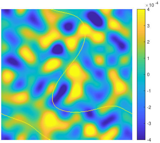
The choice of anchor points depends on the geometry of the surface, including the number of irreducible components. For arbitrary training samples, we can estimate the unknowns $\mathbf{F}$ in (47) from the linear relations

$\displaystyle\underbrace{\left[\mathbf{y}_{1},..\mathbf{y}_{P}\right]}_{\mathbf{Y}}$

$\displaystyle=$

$\displaystyle\mathbf{F}~\underbrace{[\bm{\alpha}(\mathbf{x}_{1}),\ldots,\bm{\alpha}(\mathbf{x}_{P})]}_{\mathbf{Z}}$

(48)

as $\mathbf{F}=\mathbf{Y}\mathbf{Z}^{H}\left(\mathbf{Z}\mathbf{Z}^{H}\right)^{{\dagger}}$. The above recovery is exact when we have $N=r$ achor points because $\mathbf{Z}$ has full column rank in this case. The reason why $\mathbf{Z}$ has full column rank is due to (44) and (45). Equation (44) suggests that ${\rm{rank}}(\mathbf{Z})\geq N$, while equation (45) shows ${\rm{rank}}(\mathbf{Z})\leq N$. Therefore, we have ${\rm{rank}}(\mathbf{Z})=N$, indicating that $\mathbf{Z}$ has full rank in this case. When $N>r$, the $\mathbf{F}$ is obtained using the pseudo-inverse, which is based on the least square approximation.

References

- [1] Aim@shape, digital shape workbench. http://www.infra-visionair.eu/.
- [2] H. K. Aggarwal, M. P. Mani, and M. Jacob, Modl: Model-based deep learning architecture for inverse problems, IEEE transactions on medical imaging, 38 (2018), pp. 394–405.
- [3] M. Atiyah and I. MacDonald, Introduction To Commutative Algebra, Addison-Wesley series in mathematics, Avalon Publishing, 1994.
- [4] M. Belkin, P. Niyogi, and V. Sindhwani, Manifold regularization: A geometric framework for learning from labeled and unlabeled examples, Journal of machine learning research, 7 (2006), pp. 2399–2434.
- [5] O. Bernard, D. Friboulet, P. Thévenaz, and M. Unser, Variational b-spline level-set: a linear filtering approach for fast deformable model evolution, IEEE Transactions on Image Processing, 18 (2009), pp. 1179–1191.
- [6] A. Buades, B. Coll, and J.-M. Morel, Non-local means denoising, Image Processing On Line, 1 (2011), pp. 208–212.
- [7] Y. Cho and L. K. Saul, Kernel methods for deep learning, in Advances in neural information processing systems, 2009, pp. 342–350.
- [8] K. Dabov, A. Foi, V. Katkovnik, and K. Egiazarian, Image denoising with block-matching and 3D filtering, in Image Processing: Algorithms and Systems, Neural Networks, and Machine Learning, N. M. Nasrabadi, S. A. Rizvi, E. R. Dougherty, J. T. Astola, and K. O. Egiazarian, eds., vol. 6064, International Society for Optics and Photonics, SPIE, 2006, pp. 354 – 365.
- [9] M. Elad and M. Aharon, Image denoising via sparse and redundant representations over learned dictionaries, IEEE Transactions on Image processing, 15 (2006), pp. 3736–3745.
- [10] H. Federer, Geometric measure theory, Springer, 2014.
- [11] C. Fefferman, S. Mitter, and H. Narayanan, Testing the manifold hypothesis, Journal of the American Mathematical Society, 29 (2016), pp. 983–1049.
- [12] M. Fornasier, H. Rauhut, and R. Ward, Low-rank matrix recovery via iteratively reweighted least squares minimization, SIAM Journal on Optimization, 21 (2011), pp. 1614–1640.
- [13] V. Gallese, The roots of empathy: the shared manifold hypothesis and the neural basis of intersubjectivity, Psychopathology, 36 (2003), pp. 171–180.
- [14] K. Gedalyahu and Y. C. Eldar, Time-delay estimation from low-rate samples: A union of subspaces approach, IEEE Transactions on Signal Processing, 58 (2010), pp. 3017–3031.
- [15] R. C. Gunning and H. Rossi, Analytic functions of several complex variables, vol. 368, American Mathematical Soc., 2009.
- [16] T. Hastie, R. Tibshirani, J. Friedman, and J. Franklin, The elements of statistical learning: data mining, inference and prediction, The Mathematical Intelligencer, 27 (2005), pp. 83–85.
- [17] A. S. Jackson, A. Bulat, V. Argyriou, and G. Tzimiropoulos, Large pose 3d face reconstruction from a single image via direct volumetric cnn regression, in Proceedings of the IEEE International Conference on Computer Vision, 2017, pp. 1031–1039.
- [18] M. Jacob, T. Blu, and M. Unser, Efficient energies and algorithms for parametric snakes, IEEE transactions on image processing, 13 (2004), pp. 1231–1244.
- [19] C. Koulamas and G. J. Kyparisis, Single-machine and two-machine flowshop scheduling with general learning functions, European Journal of Operational Research, 178 (2007), pp. 402–407.
- [20] Y. LeCun, C. Cortes, and C. Burges, Mnist handwritten digit database, ATT Labs [Online]. Available: http://yann. lecun. com/exdb/mnist, 2 (2010).
- [21] C. Li, C. Xu, C. Gui, and M. D. Fox, Distance regularized level set evolution and its application to image segmentation, IEEE transactions on image processing, 19 (2010), pp. 3243–3254.
- [22] T. Li, A. Krupa, and C. Collewet, A robust parametric active contour based on fourier descriptors, in 2011 18th IEEE International Conference on Image Processing, IEEE, 2011, pp. 1037–1040.
- [23] Y. M. Lu and M. N. Do, A theory for sampling signals from a union of subspaces, IEEE transactions on signal processing, 56 (2008), pp. 2334–2345.
- [24] J. Mairal, P. Koniusz, Z. Harchaoui, and C. Schmid, Convolutional kernel networks, in Advances in neural information processing systems, 2014, pp. 2627–2635.
- [25] M. Mishali, Y. C. Eldar, and A. J. Elron, Xampling: Signal acquisition and processing in union of subspaces, IEEE Transactions on Signal Processing, 59 (2011), pp. 4719–4734.
- [26] K. Mohan and M. Fazel, Iterative reweighted algorithms for matrix rank minimization, The Journal of Machine Learning Research, 13 (2012), pp. 3441–3473.
- [27] Y. Q. Mohsin, S. G. Lingala, E. DiBella, and M. Jacob, Accelerated dynamic mri using patch regularization for implicit motion compensation, Magnetic resonance in medicine, 77 (2017), pp. 1238–1248.
- [28] K.-R. Muller, S. Mika, G. Ratsch, K. Tsuda, and B. Scholkopf, An introduction to kernel-based learning algorithms, IEEE transactions on neural networks, 12 (2001), pp. 181–201.
- [29] U. Nakarmi, Y. Wang, J. Lyu, D. Liang, and L. Ying, A kernel-based low-rank (klr) model for low-dimensional manifold recovery in highly accelerated dynamic mri, IEEE transactions on medical imaging, 36 (2017), pp. 2297–2307.
- [30] G. Ongie and M. Jacob, Off-the-grid recovery of piecewise constant images from few fourier samples, SIAM Journal on Imaging Sciences, 9 (2016), pp. 1004–1041.
- [31] G. Ongie, R. Willett, R. D. Nowak, and L. Balzano, Algebraic variety models for high-rank matrix completion, arXiv preprint arXiv:1703.09631, (2017).
- [32] S. Osher and R. P. Fedkiw, Level set methods: an overview and some recent results, Journal of Computational physics, 169 (2001), pp. 463–502.
- [33] H. Pan, T. Blu, and P. L. Dragotti, Sampling curves with finite rate of innovation, IEEE Transactions on Signal Processing, 62 (2013), pp. 458–471.
- [34] G. Peyré and S. Mallat, Surface compression with geometric bandelets, ACM Transactions on Graphics (TOG), 24 (2005), pp. 601–608.
- [35] G. Pillonetto, F. Dinuzzo, T. Chen, G. De Nicolao, and L. Ljung, Kernel methods in system identification, machine learning and function estimation: A survey, Automatica, 50 (2014), pp. 657–682.
- [36] S. Poddar and M. Jacob, Dynamic mri using smoothness regularization on manifolds (storm), IEEE transactions on medical imaging, 35 (2015), pp. 1106–1115.
- [37] , Recovery of noisy points on bandlimited surfaces: Kernel methods re-explained, in 2018 IEEE International Conference on Acoustics, Speech and Signal Processing (ICASSP), IEEE, 2018, pp. 4024 – 4028.
- [38] , Recovery of point clouds on surfaces: Application to image reconstruction, in Biomedical Imaging (ISBI 2018), 2018 IEEE 15th International Symposium on, IEEE, 2018, pp. 1272–1275.
- [39] S. Poddar, Y. Q. Mohsin, D. Ansah, B. Thattaliyath, R. Ashwath, and M. Jacob, Manifold recovery using kernel low-rank regularization: application to dynamic imaging, IEEE Transactions on Computational Imaging, 5 (2019), pp. 478–491.
- [40] D. Potts and G. Steidl, Fourier reconstruction of functions from their nonstandard sampled radon transform, Journal of Fourier Analysis and Applications, 8 (2002), pp. 513–534.
- [41] M. Rauth and T. Strohmer, Smooth approximation of potential fields from noisy scattered data, Geophysics, 63 (1998), pp. 85–94.
- [42] S. Ravishankar and Y. Bresler, Learning doubly sparse transforms for images, IEEE Transactions on Image Processing, 22 (2013), pp. 4598–4612.
- [43] M. Rousson and N. Paragios, Shape priors for level set representations, in European Conference on Computer Vision, Springer, 2002, pp. 78–92.
- [44] P. Sajda, A. Laine, and Y. Zeevi, Multi-resolution and wavelet representations for identifying signatures of disease, Disease markers, 18 (2002), pp. 339–363.
- [45] B. Schölkopf and A. J. Smola, Learning with kernels: support vector machines, regularization, optimization, and beyond, MIT press, 2002.
- [46] F. Schroff, A. Criminisi, and A. Zisserman, Object class segmentation using random forests., in BMVC, 2008, pp. 1–10.
- [47] H. Shao, A. Kumar, and P. Thomas Fletcher, The riemannian geometry of deep generative models, in Proceedings of the IEEE Conference on Computer Vision and Pattern Recognition Workshops, 2018, pp. 315–323.
- [48] A. J. Smola and R. Kondor, Kernels and regularization on graphs, in Learning theory and kernel machines, Springer, 2003, pp. 144–158.
- [49] T. Sørevik and M. A. Nome, Trigonometric interpolation on lattice grids, BIT Numerical Mathematics, 56 (2016), pp. 341–356.
- [50] T. Strohmer, Computationally attractive reconstruction of bandlimited images from irregular samples, IEEE Transactions on image processing, 6 (1997), pp. 540–548.
- [51] T. Strohmer, T. Binder, and M. Sussner, How to recover smooth object boundaries in noisy medical images, in Proceedings of 3rd IEEE International Conference on Image Processing, vol. 1, IEEE, 1996, pp. 331–334.
- [52] C. Tian, Y. Xu, L. Fei, J. Wang, J. Wen, and N. Luo, Enhanced cnn for image denoising, CAAI Transactions on Intelligence Technology, 4 (2019), pp. 17–23.
- [53] M. C. Tsakiris and R. Vidal, Algebraic clustering of affine subspaces, IEEE transactions on pattern analysis and machine intelligence, 40 (2017), pp. 482–489.
- [54] S. Wang and M. Y. Wang, Radial basis functions and level set method for structural topology optimization, International journal for numerical methods in engineering, 65 (2006), pp. 2060–2090.
- [55] F. Weisz, Summability of multi-dimensional trigonometric fourier series, Surv. Approx. Theory, 7 (2012), pp. 1–179.
- [56] Z. Yang and M. Jacob, Nonlocal regularization of inverse problems: a unified variational framework, IEEE Transactions on Image Processing, 22 (2012), pp. 3192–3203.
- [57] J. Zhang, G. G. Walter, Y. Miao, and W. N. W. Lee, Wavelet neural networks for function learning, IEEE transactions on Signal Processing, 43 (1995), pp. 1485–1497.
- [58] K. Zhang, W. Zuo, Y. Chen, D. Meng, and L. Zhang, Beyond a gaussian denoiser: Residual learning of deep cnn for image denoising, IEEE Transactions on Image Processing, 26 (2017), pp. 3142–3155.
- [59] Q. Zou and M. Jacob, Sampling of surfaces and learning functions in high dimensions, in ICASSP 2020-2020 IEEE International Conference on Acoustics, Speech and Signal Processing (ICASSP), IEEE, 2020, pp. 8354–8358.
- [60] Q. Zou, S. Poddar, and M. Jacob, Sampling of planar curves: Theory and fast algorithms, IEEE Transactions on Signal Processing, 67 (2019), pp. 6455–6467.