A minimal model of many body localization
Abstract
We present a fully analytical description of a many body localization (MBL) transition in a microscopically defined model. Its Hamiltonian is the sum of one- and two-body operators, where both contributions obey a maximum-entropy principle and have no symmetries except hermiticity (not even particle number conservation). These two criteria paraphrase that our system is a variant of the Sachdev-Ye-Kitaev (SYK) model. We will demonstrate how this simple ‘zero-dimensional’ system displays numerous features seen in more complex realizations of MBL. Specifically, it shows a transition between an ergodic and a localized phase, and non-trivial wave function statistics indicating the presence of ‘non-ergodic extended states’. We check our analytical description of these phenomena by parameter free comparison to high performance numerics for systems of up to fermions. In this way, our study becomes a testbed for concepts of high-dimensional quantum localization, previously applied to synthetic systems such as Cayley trees or random regular graphs. We believe that this is the first many body system for which an effective theory is derived and solved from first principles. The hope is that the novel analytical concepts developed in this study may become a stepping stone for the description of MBL in more complex systems.
pacs
05.45.Mt, 72.15.Rn, 71.30.+hI Introduction
Quantum wave functions subject to strong static randomness may show non-ergodic localized behavior. To date, we distinguish between two broad universality classes of quantum localization: Anderson localization Anderson in low dimensional single particle systems, and many body localization (MBL) in random many particle systems BaskoAleinerAltshuler; Mirlin. In principle, there is no fundamental distinction between these two. They both reflect the lack of ergodicity of wave functions on random lattices due to massive quantum interference. However, the all important difference is that in the former case the lattice structure is defined by a low dimensional solid and in the latter by the high dimensional Fock space lattice formed by the occupation number states of a many particle system.
Many body localization is traditionally discussed in the context of spatially extended many body systems, such as interacting quasi one-dimensional electron systems BaskoAleinerAltshuler; Mirlin, or random spin chains spin1; Huse2010; Moore2012; spin5; spin3; spin2; ImbriePRL2016; ImbrieJStatPhys2016; TorresSantos17; Laflorencie19. However, that spatial extension is an added layer of complexity to a problem that manifests itself already in spatially confined geometries — a competition between ‘hopping’ and ‘randomness’ on the complex lattice structure defined by an interacting particle problem. In fact, there appears to be a paradigm shift in the field away from studying the quantum critical phenomena of the localization transition in extended systems towards manifestations of MBL in systems of mesoscopic extension, such as interacting quantum dots AltshulerGefenKamenevLevitov97; Silvestrov97; Silvestrov98; GornyMirlinPolyakov16; GornyMirlinPolyakovBurin17, small sized optical lattices RubioAbadal19; Choi16; Schreiber15, or small sized superconducting qubit arrays kai18; roushan17. This development is driven in part by pragmatism. The explosion of Fock space dimensions with increasing system size makes numerical access infamously hard and classical computers may never be powerful enough to probe the scaling regime of the MBL transition with sufficient reliability. Another motivation lies in the fascinating and only partly understood physics of localization in many body systems of intermediate size.
At this point, even basic aspects of MBL remain enigmatic, including in small sized systems. Among these, one of the most controversial topics concerns the presence or absence of a phase of non-ergodic but extended (NEE) states intermediate between the regime of ergodic wave functions at weak and localized wave functions at strong disorder. If existent, such a phase must be born out of the main principles distinguishing MBL from low dimensional AL: the high coordination number of ‘Fock space lattices’, the strong correlation of their disorder potentials, and the sparsity of the hopping matrix elements in Fock space (see the next section for a more detailed discussion). Reflecting the complexity of the problem, the physics of NEE states is often discussed for synthetic NonE_Ex; Biroli18; Mirlin1; TikhonovMirlin19_2; faoro or phenomenological models RPmodel1, sidestepping one or several of the above complications. (However, even for these, the existence of NEE phases is discussed controversially.)
Clearly, a numerically and analytically solvable minimal model defined by a microscopic Hamiltonian would provide an important contribution to our understanding of MBL. It would provide a testbed for the validity of analytical approaches by comparison to numerical diagonalization and might turn into a building block in the study of more complex systems. In this paper, we report on the definition and solution of such a system. Here, the term ‘solution’ refers to the following: (a) the construction of an effective theory of the microscopically defined system by parametrically controlled approximation, (b) the computation of observables (many body wave function, and spectral statistics) from that theory, and (c) parameter free comparison to numerics. In this hierarchy, the perhaps most important element is (a). The effective theory we derive assumes the form of a matrix-path integral in Fock space, see Eq. (45) for an impression. From this representation, observables can be extracted by powerful methods developed in the localization theory of high dimensional lattices. (For a pioneering previous comparison between analytical and numerical results for a concrete model system we refer to Ref. LeyronasSilvestrovBeenakker2000. However, that work was based on scaling theory for a specific class of observables. Lacking element (a), it did not have the scope of the present analysis.)
The model we consider is implicitly defined by the following criteria: its Hamiltonian contains the sum of a one-body and a two-body part. Both are maximally entropic and have no symmetries besides hermiticity (not even particle number conservation). In the non-interacting case, , the product eigenstates of define a basis in which the system is trivially localized. The Hamiltonian acts as a ‘hopping operator’ and at a critical strength will induce a many body localization transition. In a manner detailed in the next section, the criteria listed above state that is the Majorana SYK Hamiltonian.
The maximum entropy criterion makes the SYK model much simpler than MBL systems with spatial extension. At the same time, it displays a wealth of phenomena characteristic for MBL. Foremost among these is a change from delocalized to localized behavior. For finite , this is a crossover. However, the exponential dependence of the Fock space lattice extension on implies that it rapidly acquires signatures of a transition as increases. Second, the model supports a regime (not a phase) of NEE states prior to the onset of localization. We will discuss how the diminishing support of these states upon approaching the transition reflects the structure of the system’s Fock space, and how this differs from phenomenological models. However, the most important point of all is that the spectral and wave function statistics of the model can be computed analytically and that these results can be numerically tested in a parameter free comparison. The analytical approach is based on matrix integral techniques imported from the theory of high dimensional random lattices. We apply these techniques subject to a number of assumptions which should generalize to other many body systems of small spatial extension and/or a high degree of connectivity. We, therefore, hope that the approach discussed in this paper may become a stepping stone for the solution of more complex manifestations of MBL.
Plan of the paper: In the next section, we introduce our model system, qualitatively discuss its physics, and summarize our main results. The remaining parts of the paper discuss the derivation of these findings, where we try to keep the technical level at a bare minimum. In Section III we map the computation of disorder averaged correlation functions onto that of an equivalent matrix integral. In Section IV, a stationary phase approach is applied to reduce the matrix integral to an effective theory describing physics at large time scales. In sections V and VI we apply this representation to the discussion of wave function statistics and the localization transition, respectively. We conclude in Section VII with a discussion comparing our results to those obtained for other models, and on possible generalizations to other MBL systems. Technical parts of our analysis are relegated to a number of appendices.
II Model and summary of results
In this section, we first introduce the SYK model and then discuss its physics of quantum localization in qualitative terms. Much of this outline is formulated in general terms which should carry over to similar models. In the remaining parts of the section we get more concrete and summarize our results in comparison to numerics.
II.0.1 SYK Model
The SYK Hamiltonian SYK1; SYK2
| (1) |
describes a system of Majorana fermions, , subject to an all-to-all interaction, with matrix elements drawn from a Gaussian distribution of variance . Defined in this way, it defines an ideal of a massively interacting quantum system lacking any degree of internal structure. Due to the ‘least information’ principle realized through the stochastic interaction, all single particle orbitals, , stand on equal footing, and the absence of a continuous -symmetry prevents the fragmentation of the Fock space into sectors of conserved particle number. Reflecting these features, the physics of the SYK Hamiltonian at large time scales becomes equivalent to that of random matrix theory (RMT), with wave functions homogeneously distributed over the full Hilbert space.
A tendency to Fock space localization is included by adding to a free particle contribution SYK_GG; Shepelyansky17,
| (2) |
with a likewise random antisymmetric matrix , with matrix elements drawn from a Gaussian of variance . Without loss of generality, we may assume to be diagonalized into a form , where are the eigenvalues of the hermitian matrix . For the above distribution of the matrix elements these eigenvalues are random numbers with variance .
We next translate from the Majorana many body Hamiltonian formulation to one in terms of a fermion Fock space (lattice). To this end, define complex fermion annihilation operators satisfying . With the number operators , we then have
| (3) |
Representing this Hamiltonian in the basis of occupation number states, , , it assumes the form of a random potential on the hypercube defined by all sites fn2. In the same basis, the interaction, , assumes the role of a fermion number conserving ‘hopping operator’ connecting sites of bit separation 2 and 4 fn1. This hopping introduces a complex connectivity pattern on the two decoupled sublattices of definite (even, say) parity, containing
| (4) |
sites each. Fig. 1 illustrates this structure for a Fock space of Majorana fermions. The lines indicate the states connected to the arbitrarily chosen site . Notice the high coordination number and the absence of lattice periodicity, symptomatic for this and for other Fock space lattices. The competition between the localizing random potential and the delocalizing hopping defines the MBL problem, regardless of their detailed realization.

II.1 Qualitative discussion
In this section, we discuss the physics of the above random system in qualitative terms. Specific topics include the existence of a localization-delocalization transition, its signatures in spectral and wave function statistics, and a regime of non-ergodically extended states. Most parts of this discussion do not make specific reference to the SYK model and should equally apply to other systems.
The single most important system quantity relevant to the understanding of the above observables at a specific energy, say, , is the local density of states in Fock space,
| (5) |
where , and indicates that we consider averaged over realizations of , but at a single realization of . (The discussion above shows that the large coordination number of the lattice makes a largely self-averaging quantity. Averaging over is largely a matter of technical convenience.) From the perspective of site , the large number of nearest neighbors represents an environment and, on this basis, one expects a Lorentzian profile
| (6) |
where we have set for definiteness, and the broadening must be self-consistently determined (cf. Eq. (35) below) in dependence on the following parameters:
- •
the many body band width, , of the interaction operator ( fn3 for the SYK Hamiltonian, ),
- •
- •
The number of nearest neighbors, , connected to Fock space sites, , by the interaction . ( for the SYK Hamiltonian.)
On this basis, we must distinguish between four regimes of qualitatively different level hybridization, :
- I:
: In this regime, the band width is below that of . The on-site randomness is largely irrelevant and states are ergodically spread over the full Fock space lattice. Hybridization of levels over the full band width implies .
- II:
: The band width exceeds implying that the majority of sites become inaccessible. States of fixed energy now populate only a fraction of Hilbert space sites. However, for a given site with energy inside the accessible window , the hopping nearest neighbors have accessible energy , and thus are also accessible. As a consequence, for all sites with energy .
- III:
: In this regime, the energetic separation even between nearest neighbors exceeds the interaction band width. In the consequence, the hybridization of levels with energy is suppressed down to , and the band of accessible sites narrows to this width. For a given site inside the resonant window, nearest neighbors of energy typically lie outside it. However, a fraction of the nearest neighbors does satisfy the resonance condition. With neighbors, this gives a number of of hybridizing partner sites, which safeguards the extension of states.
- IV:
: The number of nearest neighbors satisfying the resonance condition becomes lesser than unity which implies strong localization of states in Fock space.
The regimes I-IV cover the entire spectrum from fully extended states, I, over ‘non-ergodically’ extended (NEE) states II,III, to localization IV. (In regimes II,III states cover only a fraction of the Fock space sites. In this paper, we are following the convention to call such non-uniformly distributed states ‘non-ergodic’. This is a misnomer in that the states do remain uniformly distributed over an ‘energy shell’ of resonant sites.) The level broadening characterizing the local spectral density in the respective regimes is described by the universal formula
| (7) |
where the value of the hybridization parameter and the corresponding disorder strengths are summarized in table 1.
| regime | disorder, | level broadening, | spectral statistics | state extension | |
|---|---|---|---|---|---|
| I | RMT | Wigner-Dyson | |||
| II | NEE1 | Wigner-Dyson | |||
| III | NEE2 | Wigner-Dyson | |||
| IV | localization | Poisson |
Before leaving this section, it is worthwhile to comment on various phenomenological approaches to MBL. We distinguish between three categories of phenomenological formulations. The ‘most phenomenological’ class models Fock space by a random matrix. For example, the Rosenzweig-Porter (RP) model contains a Gaussian distributed random matrix (as a proxy of the interaction operator, ) perturbed by a likewise random diagonal representing RPmodel; RPmodel1. The second class replaces Fock space by a high dimensional synthetic lattice, such as the Bethe lattice Zirnbauer86; NonE_Ex; Biroli18, or a random regular graph Mirlin1; TikhonovMirlin19_2; Lemarie17; Lemarie20. Finally, there is the random energy model (REM) which retains the microscopic structure of Fock space but replaces the amplitudes by uncorrelated random variables (see our previous publication NEE_SYK for an application of this idea to the SYK Hamiltonian). These models are designed to mimic specific aspects of localization and wave function statistics in high dimensional environments. However, they fall short of describing the characteristic correlations between site energies and high lattice coordination number essential to the distinction of the regimes I-IV and their statistical properties reviewed in the next section.
One of the main messages of this paper is that the analytical theory for ‘real’ systems need not be more difficult than that for synthetic models. What at first sight looks like a complication — the combination of high coordination numbers and correlations in the microscopic Fock space — actually is a resource and leads to self averaging (a source of simplicity) at several stages of our computations below.
On this basis, we now discuss quantitative results obtained for the description of regimes I-IV. For notational simplicity, we work in units where the variance of the matrix elements equals . At this value, the band width of the interaction operator .
II.2 Spectral statistics
We describe the statistics of the system’s many body spectrum in terms of the spectral two point correlation function at the band center
| (8) |
where with is the averaged many body density of states at zero energy and the subscript stands for the cumulative average .
Regimes I-III: In these regimes, wave functions are extended and their eigenenergies are correlated and described by Wigner-Dyson statistics. Assuming an odd number of complex fermions (for which the SYK model is in the unitary symmetry class A), this reflects in the spectral statistics of the Gaussian unitary ensemble (GUE),
| (9) |
where is the average density of states. With the local densities given by Eq. (6), and the distributed over a range , we find
where, here and throughout, represents numerical constants. The second line of Eq. (II.2) states that in the regimes of intermediate disorder strength, only a fraction of active sites contributes to the spectral support of wave functions.
Regime IV: In the regime of strongly localized states, eigenenergies become uncorrelated and we expect Poisson statistics. In this paper, we will use the change from Wigner-Dyson to Poisson statistics as one of two indicators for the Anderson transition at the boundary between regimes III and IV. Referring for a more detailed discussion of the localization transition to Section II.4 below, we note that in the literature Huse10, the difference between the two types of statistics is often monitored by analysis of -ratios Huse07, i.e. numerical comparison of the ratios between nearest neighbor many body energy levels, , with the expected ratios for Poisson and Wigner-Dyson statistics. However, we have observed that naked eye comparisons can easily trick one into premature and qualitatively wrong conclusions. Instead, we adopt a more sophisticated entropic procedure detailed in Sec. V.3 and compute Kullback-Leibler divergences, where the latter are defined as relative entropies of the numerically observed distribution to the Poisson and Wigner-Dyson distribution, respectively. The panel (b) of Fig. 3 shows how this entropic measure changes abruptly at the localization transition.
II.3 Wave function statistics
The second class of observables considered in this paper are the moments of wave functions of zero energy, ,
| (12) |
The statistics of these moments not only indicates the localization transition but, unlike spectral statistics, also differentiates between the three weak disorder regimes I-III.
Regime I: wave functions are ergodically distributed over the full Fock space, with moments given by those of the Porter-Thomas distribution,
| (13) |
otherwise found for the wave functions of random matrix Hamiltonians. The result states that the complex amplitudes are independently distributed Gaussian random variables.
Regimes II & III: The wave functions no longer ergodically occupy the full Fock space. The bulk of their support is concentrated on the subset of resonant sites, . This behavior reflects in the moments
| (14) |
where . To make the connection of this expression to Eq. (13) more transparent, consider the case of large , where
| (15) | ||||
These moments again coincide with those of a Gaussian distribution, now defined on the diminished number of resonant sites in Fock space, over which the wave functions are uniformly spread.
Noting that , , the dependence of on is approximated as
| (18) |
This suggests an interpretation in terms of a ‘fractal’ whose dimension differs from the naive dimension by a factor , rather than the more usual with some . Alternatively, we may interpret the wave functions as ergodically, or thermally extended over an ‘energy shell’ of sites defined by the condition .
Figures 4 and 5 show a comparison of our analytical predictions for the wave function moments dependence on (Fig. 4), respectively and (Fig. 5), to numerical simulations for Majorana fermions. Vertical dashed lines in Fig. 4 mark the boundaries between different regimes, and is the scale at which Fock space localization sets in, see Eq. (19) and the refined expression, Eq. (83), accounting for corrections. For the numerically accessible -values, regime II, , lacks the width required for the comparison with power laws and we concentrate on regime III. Given that there is no fitting of numerical parameters and numerical error bars are smaller than symbol size, the comparison is good. We notice a slight deviation in the -scaling, increasing for large moments, . However, this mismatch does not show consistent system size dependence, and we cannot attribute a clear trend to it. Starting from we also see deviations of the predicted -scaling at large values, which is a first indication of the proximity of the Anderson transition. At first sight, it may seem paradoxical that these signatures are first seen for larger , where the parametric dependence of the localization threshold increases in . However, the situation becomes clearer when we represent the inverse participation data as a function of a scaled parameter, as we will discuss next.
II.4 Strong localization
The wave functions describing random hopping on a lattice are localized on small sized clusters if, statistically, the nearest neighbor hopping matrix elements become smaller than the variations of the local site energies. In this work, we numerically and analytically compute the threshold strength of the disorder where this happens.
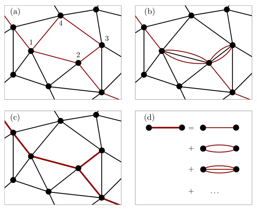
Analytical approach: Above, we reasoned that the problem of MBL is defined by a competition of localizing on-site disorder and delocalizing hopping in a complex high-dimensional lattice. Unlike in previous work on Anderson localization in high dimensions, which is formulated on simplified synthetic lattice structures such as the Bethe lattices Kravtsov2; Biroli17 or random regular graphs Kravtsov2; Biroli12; Kravtsov1; DeLuca14, we here directly work in Fock space. What helps to keep this more complicated problem under control is the huge effective lattice coordination number of , and a simplification known as the ‘effective medium approximation’ Efetov. This approximation is commonly applied in the discussion of Anderson localization on high dimensional lattices and backed by their large coordination numbers. It describes transport as a process avoiding local loops (see Fig. 6), while multiple link traversals (panel (a)) are included. The rationale behind this simplification is that at any given order in hopping perturbation theory, amplitudes with the lowest number of statistically independent energy denominators contribute the strongest. Its application to the SYK lattice, detailed in Section VI, sums these processes via recursion relations (such as Eq. (51)) whose solution leads to prediction Eq. (83) for the critical disorder strength. For large this formula simplifies to
| (19) |
The characteristic scaling was first predicted in Ref. AltshulerGefenKamenevLevitov97, where the logarithmic correction relative to the naive estimate mentioned in the introduction accounts for resonant hybridization with sites beyond nearest neighbors.
However, our aim here is to compare to the real world of small sized systems where things get more complicated. For one, the difference between the asymptotic result and the more precise expression Eq. (83) becomes noticeable. Second, various approximations in the execution of the effective medium program rely on the largeness of and again may lead to errors in terms sub-leading in . These uncertainties must be kept in mind when we compare to the numerical computation of the threshold.
Numerical approach: As indicated above, we detect the onset of localization via two indicators. The first is the wave function statistics, where serves as a transition order parameter jumping between the values in the ergodic weak disorder regime to in the localized phase. Here, the first value must be taken with a grain of salt, again due to finite system size. Our discussion in the previous section shows that before reaching the transition, in regimes II, III, we have deviations away from the ergodic limit . In the thermodynamic limit, these are inessential (because is exponential in while the corrections of Eq. (15) are in powers of .) However, for system sizes in numerical reach, we cannot expect an actual jump in the order parameter. The best one can hope for is gradual steepening of the curve for upon increasing system size.
The second diagnostic is spectral statistics, where we monitor the proximity to a Wigner-Dyson or Poisson distribution via the Kullback-Leibler entropy as discussed in Section V.1. Ideally, one would hope that both signatures, inverse participation ratio and spectral statistics reveal a phase transition via a crossing point when subjected to appropriate finite size scaling, and that these crossing points sit at the same value. In reality, we almost, but not fully observe this behavior. In Fig. 3, we show the inverse participation ratio , and the Kullback-Leibler entropy as a function of the scaled variable, , where is given by the analytical prediction Eq. (83) in terms of the Lambert -function. We observe that (i) both observables show reasonably well defined crossings with a tendency of sharpening behavior for increasing system size, however, (ii) these crossings deviate from the analytically predicted value by a numerical factor of , and by a factor of similar magnitude among themselves. Turning to different scaling variables, one may sharpen the finite size scaling of either one of the two observables. For example, the inset in the first panel shows as a function of , with from Eq. (19) with two numerical parameters outside and inside the ‘log’ adjusted to improve visibility of the crossing point crossing. However, this comes at the expense of a more diffuse scaling of the entropy, as shown in the inset of the second panel. We observe that the numerically obtained scaling for small systems responds sensitively to the finite corrections (Eq. (83) vs. Eq. (19)).
All in all, we consider the agreement with the numerics quite favorable. We see clear evidence of critical behavior in two observables and the position of the transition is obtained without free fit parameters from the analytical solution of an effective lattice model. This may be the first genuine Fock space localization problem where a first principle solution of this kind has been possible.
In the next sections, we discuss the derivation of the analytical results mentioned above. Hoping that elements of this computation might become blueprints for the analysis of other models of MBL, we try to be as pedagogical as we can. Various technical details are relegated to appendices.
III Matrix model
We start the derivation of the results summarized above by constructing an exact matrix integral representation of the correlation functions introduced above to describe many body wave functions and spectra. The unconventional perspective of this approach is that there will be no second quantized representation of Fock space: we think of the SYK Hamiltonian as a big matrix, and treat it like that. In this section, we discuss the construction of a matrix integral representing the theory averaged over disorder. The physics behind this formulation and that of a subsequent stationary phase analysis of the theory will be discussed in the next section.
All information on spectra and wave functions of the system is contained in the Fock space matrix elements of resolvent operators,
| (20) |
where and, here and throughout, is infinitesimal (with a limit to be taken in the final step of all calculations). Specifically, the correlation functions above are obtained as
| (21) |
where is computed at , and denotes the average over coupling constants of .
Construction of the matrix integral. — Following standard protocols, we raise the Green functions to an exponential representation before performing the Gaussian average. The basic auxiliary formula in this context is , where is a general matrix and the dimensional ‘graded’ vector contains -commuting components , and an equal number of Grassmann components . The double integral over these variables cancels unwanted determinants , while the pre-exponential factors, either commuting or anti-commuting, , isolate the inverse matrix element. With the identification , we are led to consider the generating function
| (22) |
Here, , contains the energy arguments of the Green functions and is a Pauli matrix distinguishing between advanced and retarded components. The matrix acts as a source for the generation of the required moments of Green function matrix elements. Specifically, we define
| (23) | ||||
| (24) |
where is a projector onto commuting and anticommuting-variables, respectively, , and projects in causal space, , . With these definitions, an elementary computation shows that
| (25) | ||||
| (26) |
with . In the following, we consider the sources absorbed in a redefined energy matrix, , and remember their presence only when needed.
At this point, the averaging over can be performed, and it generates a quartic term
| (27) |
where we defined for the scaled variance of the SYK Hamiltonian , ,
| (28) |
and with . We next perform an innocuous but physically meaningful (see next section) rearrangement , where the supertrace Efetov accounts for the minus sign caught when exchanging anti-commuting variables. The next step is a Hubbard-Stratonovich transformation decoupling the matrices in terms of auxiliary matrix fields . Referring for details of the procedure to Appendix A we note that after the decoupling the integral over -variables has become Gaussian and can be carried out. A more interesting statement is that of the Hubbard-Stratonovich fields , all but one can be removed, too, by straightforward Gaussian integration. Upon restricting to this leaves us with a single integration,
| (29) | ||||
over a dimensional matrix carrying indices in causal space, super-space, and Fock space. The information on the SYK system now sits in the site-diagonal one-body term, , and the hopping operator which represents the interaction and acts on matrices in Fock space as
| (30) |
Finally, represents the band width, which we have set to unity. To simplify formulas, we will consider energies , scaled by this parameter, and suppress it throughout.
Discussion of the matrix integral. — This is now a good point to discuss the meaning of the above Hubbard-Stratonovich transformation and of the matrix-representation. The two-fermion vertices entering the theory after disorder averaging describe the scattering of Fock space states off the four-Majorana operators contained in the Hamiltonian, and in this way introduce the lattice connectivity indicated in Fig. 1. While a direct analysis of individual Fock space amplitudes seems hopeless, progress can be made if the propagators are paired to two-amplitudes composites as indicated in Fig. 7. For two reasons, the pair amplitudes are more convenient degrees of freedom: First, the pair action governing scattering in the two-state channel (cf. the structure of the action (29)) is relatively easy to describe, see below. Second, the advanced/retarded combinations appear as terminal vertices in the computation of Green functions , where the dots stand for the unspecified final points of the correlation function. With the exact identity , we have , where is the density of states at the band center. The way to read this (Ward) identity is that the product of Green functions contains a singularity, provided is a structureless quantity. (The latter condition does not hold in systems with localization, where the isolated eigenstates support a point spectrum with poles rather than a uniform cut.) This argument indicates that the ‘soft mode’ is key to the understanding of observables probing spectrum and eigenfunctions of the system.
In the matrix integral framework, the above singularity shows in the presence of a soft mode in the integration over the variables . To isolate this mode, we note that Eq. (29) has an approximate symmetry
| (31) |
under rotations homogeneous in Fock space. The set of these transformations defines , i.e. the group of invertible matrices with anti-commuting entries. Invariance under this symmetry is weakly broken only by the frequency/source matrix , which, ignoring the infinitesimal sources, transforms as . This reduces the symmetry down to the transformations diagonal in advanced-retarded (-indices) space, .
The essential question now is whether the above weak explicit symmetry breaking is spontaneously broken in the matrix integral (much as a weak explicit symmetry breaking by a finite magnetic field gets upgraded to spontaneous symmetry breaking in a ferromagnetic phase.) In the latter case, we expect a soft Goldstone mode whose ‘mass’ is set by the symmetry breaking parameter, , and singularities in line with the observation above. To investigate this question and the consequences in the observables and , we next subject the theory to a stationary phase analysis.
IV Effective theory
In this section, we map the exact theory Eq. (29) to an approximate but more manageable effective theory. The conceptual steps are standard and consist of a saddle point analysis, followed by a Ginzburg-Landau style expansion (see Section VI) of the exact action in fluctuations around a homogeneous saddle point.
We have already established the presence of an exact (in the limit ) rotational soft mode isotropic in Fock space. Since much of the analysis below will focus on strong with eigenvalues of comparable to or exceeding the , we anticipate that fluctuations of lowest action cost will be commutative in the sense . We thus start from an ansatz where fluctuations are diagonal in the occupation basis. In view of the fermion parity conservation of both we focus on a sector of definite parity, chosen to be even. The locality of in the occupation number basis is in competition with the hopping described by . However, what works to our advantage is that the action of on the states is remarkably simple: thinking of as the matrix elements of a ‘density matrix’, represents a state without off-diagonal matrix elements. It is a non-trivial feature of that it preserves this structure, , i.e. the adjoint action on Fock-space diagonal matrices does not generate superpositions of off-diagonal states. A straightforward combinatorial exercise shows that (see Appendix B for details)
| (32) |
with all other matrix elements vanishing, and normalization . Notice that for a given , we have neighbors with hamming distance , connected to by . This shows distance hopping is the most important by ‘phase volume’.
With these structures in place, a variation of action (29) leads to
| (33) |
Notice that resembles times the local ‘propagator’ (see inset of Fig. 7) of site , dressed with a self energy due to hopping via to neighboring sites. It is this term which makes the stationary phase equation non-trivial. In a first step towards the solution, we neglect imaginary contributions to and focus on the local ‘spectral density’ instead. (In the effective action, the imaginary part of describes an energy shift which is inessential to our problem.) Causality requires , i.e. the sign of the self energy is dictated by that of the imaginary part contained in the energy arguments. Otherwise the saddle point equation is rotationally invariant in the internal indices of the theory. This motivates an ansatz,
| (34) |
with real coefficients . Inspection of Eq. (33) shows that these coefficients afford an interpretation as mean field local density of states.
Substituting this expression into the equation and temporarily ignoring the small energy argument, , as small compared to both and , we obtain the variational equation
| (35) | ||||
| (36) |
where denotes the matrix diagonal in the occupation basis, with elements , and where we introduce the variational level hybridization, . The structure of this equation contains the key to its solution: For , the normalization implies that it is solved by . In the chosen units, this is () the density of states at the SYK band center. For finite , the summation over implements an effective average over the connected states, which now carry random energy. In Appendix C we show that the average stabilizes the solution (37),
| (37) | ||||
| (38) |
where ‘’ stands for equality up to corrections exponentially small in . We interpret this result as the spectral density of sites with energy and decay rate into neighboring sites. The latter is finite for states below a threshold . For , the rate is given by the energy denominator of neighboring sites. In the opposite regime, , the energy denominators of states in resonance with the SYK band width are of , leading to the second line in Eq. (37).
The saddle point solutions discussed thus far are distinguished for their diagonality in all matrix indices. However, we now recall that the action is invariant under Fock space uniform rotations Eq. (31), implying that uniformly rotated saddle point configurations are solutions, too. (Technically, this follows from the cyclic invariance of the trace.) Next to this uniform Goldstone mode, configurations with site-diagonal rotations commutative with are expected to cost the least amount of action. With , this makes , the effective degrees of freedom of the theory, and substitution into Eq. (29) defines the Goldstone mode integral,
| (39) | ||||
where again denotes the matrix diagonal in the occupation basis, with elements . In the next two sections, we investigate what this integral has to say about wave function statistics and Fock space localization, respectively.
V Spectral and wave function statistics
In this section, we explore the spectral and wave function statistics in regimes I-III. The presumption is that wave functions are not yet localized and correlated with each other. This should lead to Wigner-Dyson spectral statistics and wave function moments reflecting the extended nature on the subsets of Fock space corresponding to active or resonant sites.
To test these hypothesis it is sufficient to consider the integral (39) in the presence of effectively infinitesimal explicit symmetry breaking : besides the sources, , this parameter contains a frequency argument of the order of the exponentially small inverse many body level spacing in the case of spectral statistics, Eq. (25), or the infinitesimal parameter in the case of wave function statistics, Eq. (26). On general grounds, we expect the smallness in the ‘explicit’ symmetry breaking in a Goldstone mode integral to lead to singular contributions proportional in the inverse of the that parameter after integration. (Inspection of the prefactors, in the definition of the wave function statistics shows that such singularities are actually required to obtain non-vanishing results.) These most singular contributions to the integral must come from the Goldstone mode fluctuations of least action, which are fluctuations homogeneous in Fock space,
| (40) |
With , the substitution into the action Eq.(39) leads to
| (41) |
where we made the dependence of the action on the sources required to calculate moments via Eq. (24) explicit again, and we noted .
Before proceeding, we note that the structure of this action is identical to that describing the Rosenzweig-Porter model — a single random matrix of dimension containing Gaussian distributed disorder on the matrix diagonal Ossipov. An important difference is, however, that the diagonal disorder in the latter is uncorrelated, while the Fock-space diagonal disorder induced by is highly correlated. As a consequence, the effective action for the Rosenzweig-Porter model only allows for homogenous saddle point solutions Ossipov; NEE_SYK, while here we encounter solutions that become inhomogeneous in Fock space once on-site disorder exceeds the band width. The inhomogeneity accounts for a site-dependent broadening , induced by correlations in the disorder amplitudes, and also manifests in a separation into regimes II/III of the regime of non ergodic extended states. In the following, we discuss what this reduction of the model has to say about spectral and wave function statistics.
V.1 Spectral statistics
To obtain a prediction for spectral correlations based on the representation Eq. (39) with Fock space zero mode, we consider the correlation function (8), represented through matrix integral Green functions as in Eq. (III) and Eq. (25). To compute these quantities from the effective theory, we need to expand the action Eq. (41) to lowest order in the parameter , and to second order in the sources (23). The straightforward -expansion yields (cf. Eq. (67))
| (42) |
where is the zero energy density of states, Eq. (II.2). What remains, is the source differentiation and the integration over the matrix . To get some intuition for the integral, notice that the non-linear degree of freedom affords a representation, , where contains various compact angular variables (cf. Appendix E), and
| (43) |
a rotation matrix in causal space. Diagonal in super-space, this matrix is parameterized in terms of the two ‘Bogolubov’ angles , where is a compact rotation variable, and a non-compact real variable. This representation reveals the geometry of the integration manifold as the product of a sphere () and a hyperboloid () (coupled by variables contained in .) Where the physics of non-perturbative structures in spectral and wave function statistics, and localization is concerned, the most important player is the non-compact variable, , as only this one has the capacity to produce singular results. Heuristically, one may think of the model reduced to its dependence on this variable as a non-compact version of a Heisenberg-model, containing hyperboloidal, rather than compact spins as degrees of freedom.
Referring for details of the source differentiation and the subsequent integration over the matrix Efetov to Appendix E, the above reduction of the model yields the GUE spectral correlation function (9) for the spectral statistics on scales of the many body level spacing in regimes I-III. With increasing energies, the assumption of homogeneity of fluctuations in Fock space breaks down (cf. the next section) beyond a ‘Thouless energy’ whose value depends on the specific observable under consideration fn6. However, the detailed investigation of Thouless thresholds for the present model is beyond the scope of the paper.
V.2 Wave function statistics
In the same manner, we may consider the local moments of wave functions Eq. (12), represented via Green functions Eq. (III), and obtained from the matrix integral through Eq. (26). A key feature of this expression is that it contains a limit the factor must thus be compensated for by an equally strong singularity from the integral, where couples through . Setting in Eq. (42) and integrating over the functional differentiated in sources (a calculation detailed in Appendix E), then yields the moments (13)–(15).
The support of wave functions in regimes II and III is different (as indicated by the different value of in Eqs. (15)), while the DoS Eq. (II.2) assumes the same value. The reason for this is that, in regime II, there is no distinction between active and resonant sites: there are active sites contributing with unit weight to the DoS. By contrast, in III, the dominant contribution to the DoS comes from the smaller number of resonant sites, with sharply peaked spectral weight , .
V.3 Comparison to numerics
To numerically check the predictions for the statistics of many body wave functions and spectra, we calculated eigenfunctions and spectrum from exact diagonalization of the Hamiltonian , see (1) and (3), for obtained by diagonalizing (2) as a one-body problem, for Majorana fermions and varying values of . We kept of the total spectrum and verified both a nearly constant density of states and that results remain unchanged when we restrict to a smaller energy window. From the selected eigenfunctions in the center of the band, we calculated statistics of the moments of the wave function according to Eq. (12). The eigenfunctions are normalized in each definite parity subspace. For the spectrum we compared the numerical statistical distribution with both Wigner-Dyson and Poisson distributions by calculating the Kullback-Leibler divergence, , where is the spectral statistics from numerical data and the respective distribution. In order to avoid level unfolding, we followed Ref. Huse07 and studied the statistics of ratios of energy spacings, , where is the nearest neighbor spacing of the eigenenergies . The are then given by numerically integrating either the Wigner-Dyson or the Poisson distribution for the variable over each bin centered at , given by Ref. Bogomolny13,
| (44) |
where is a numerical correction given by , with and is obtained from fitting numerical results in the GUE Bogomolny13.
In all figures the numerical values result from averaging over eigenvectors and spectrum, taken from the band center and from both parity sectors, of at least independent realizations of the model. In computing the Kullback-Leibler divergence, the numerical distribution for is obtained by splitting the interval into bins of equal widths.
VI Extended-to-localized transition
In regimes, II, III, the dominant contribution to the matrix integral at the lowest energies comes from homogeneous contributions . Upon approaching the localization threshold III/IV, inhomogeneous fluctuations gain in importance and eventually destabilize the mean field theory. To describe this physics, we need an effective action generalized for inhomogeneous fluctuations, and more manageable than Eq. (39). We derive it in Appendix D under the assumption that the sum over a large number of fluctuating terms represented by the term is largely self-averaging. An expansion to lowest order in fluctuations around the homogeneous average then leads to the effective hopping action
| (45) | ||||
| (46) | ||||
| (47) |
with and ‘’ traces only over internal degrees of freedom. Eqs. (45) and (47) are the main result of this section. Depending on the value of Eq. (37), this action describes the entire range from vanishing to large deformations . We next discuss what this action has to say on the ergodic-to-localization transition.
The key player in this problem is the hopping term (45) where matrices at -neighboring sites are coupled, subject to a weight which contains the local spectral densities. In analytic approaches to localization on high dimensional lattices, it is common to set these weights to unity. However, in view of the massive site-to-site fluctuations of we prefer not to make this assumption and work with a given realization for as long as possible. Approaching the transition from the localized side where the integration over ’s is subject to only small damping , the essential degrees of freedom are once again the non-compact variables, contained in , Eq. (43).
To better understand the significance of this structure, we write to represent the hopping part of the action as
where . Consider a situation where the accumulate hopping weights out of site are small. In this case, large fluctuations of the non-compact angles, dominate the functional integral. To understand the consequences, we note that the measure of the -integration in the angular representation is given by Efetov
where . For small typical values , the exponential weighs effectively cut off the integration over at . Individual terms in the second line of the above representation of are smaller than the accumulated weights in the first line, and so the integral can be approached by perturbative expansion in the hopping terms. As an example, consider the sixth order expansion indicated via the highlighted links in Fig. 6. Retaining only the information on the non-compact integrations , the contribution with a loop (left) and that with doubly occurring links evaluate to
| loop: | (48) | |||
| no loop: | (49) |
where the indices refer to the participating -matrices, . This estimate shows that the contribution of loops in the perturbation expansion is suppressed. At the same time, the largeness of the individual contributions signals that infinite order summations are required. The effective medium approximation achieves this summation, loops excluded. The approximation is called ‘effective medium’ because from the perspective of individual sites in Fock space the contribution of all hopping processes terminating at that site adds up to the influence of an effectively homogeneous background medium, transmissive or not depending on the strength of the couplings.

To see how this comes about, consider a site with local configuration and let be the contribution to the functional integrated over all links connected to via the neighbor , through the loopless coral like structure indicated in Fig. 8. The essence of the approximation is the recursion relation,
where the product extends over all sites, , connected to by hopping, acts as a convergence generating factor, and we defined
| (50) |
for the coupling constants weighting the hopping kernel. If we now take the product (assuming self averaging in the sense that the fully integrated amplitude, depends on the terminal site, , but not on the detailed values of the neighbor amplitudes), the equation assumes the form,
where the presence of the convergence generator is left implicit. In the deeply localized regime, , the integral decouples, and is a solution by supersymmetry (i.e. the unit normalization of all source-less integrals in the present formalism). This suggests Efetov a linearization, , where the emergence of a non-trivial solution is taken as a criterion for the localization transition. Substituting this ansatz into the equation, and again using supersymmetry, , we obtain
| (51) |
This is a linear integral equation governed by a random lattice structure in Fock space via the couplings and an internal structure encoding the randomness of the system via the -integrals. Although the integral equation may look helplessly complicated, progress is possible recalling our previous observation: we again have a situation where the integrations extend over wide parameter intervals such that the leading non-compact variable is the key player. Assuming that the solutions depend on the non-compact variable as , and referring to Ref. Zirn86 for details of the integration over remaining variables, the reduction of Eq. (51) to the regime of interest, , reads
| (52) | ||||
Ref. Zirn86 contains a pedagogical discussion of the solution of the homogeneous variant of this equation, including the somewhat subtle issue of boundary conditions. It turns out that the key to the stability of the localized solution, lies in the spectrum of the linear kernel : a spectrum with lower bound means that perturbations will grow under the application of the linearized kernel, signifying destabilization of the null solution . We thus declare the existence of a minimal eigenvalue as a delocalization criterion. Due to translational invariance in eigenstates are of the form , where the coefficients are determined by the reduced equation, , with
Substitution of the kernel in Eq. (52) followed by differentiation in shows that the positive matrix assumes its smallest values at , and the straightforward integration at that value defines the matrix,
We thus arrive at the eigen equation
| (53) | ||||
| (54) |
where the sum extends over sites in Hamming distance four to the reference site hamming, and we recall that . We read Eq. (53) as an equation for the existence of a unit eigenvalue whose solvability depends on the value of determining the local density of states, . In Appendix F we show that the summation in this equation is dominated by resonant sites, and how this simplifies its logarithmic dependence. Once again using the self averaging feature to replace the sum by an average over the distribution of , we find that Eq. (53) has a solution for determined by the criterion Eq. (83). In the limit the latter simplifies to Eq. (19). However, as discussed in section II.4, the numerical data for small values responds sensitively to such approximations and improved agreement is obtained by working with the solution Eq. (83).
VII Discussion
In this paper, we have presented a first principles analysis of Fock space localization in the Majorana SYK4+2 model, describing a competition of two-body interaction and one-body potential. Within this setting, we provided a complete description from an ergodic regime, over an intermediary regime of non-ergodic extended states to the localized phase, all formulated in the eigenbasis of the one-body Hamiltonian. Our main results are the identification of the MBL transition point, and the quantitative characterization of wave functions, particularly in regimes where they are neither localized nor trivially extended.
We compared the analytical results to numerical data for systems of size without fitting parameters. For systems of this size, the intermediate regime II is too narrow for a reliable comparison. However, in the ergodic regimes I and the strongly non-ergodic regime III we obtained good agreement between analytical and numerical results. The finite size scaling of both wave function and spectral statistics revealed an Anderson transition at a critical point which agreed with the theoretically predicted value up to a size-independent numerical constant of . In view of the numerous large approximations involved in the construction of the theory, we consider this a reassuring test for the applicability of localization theory on high dimensional lattices to realistic systems.
Conceptually, the main contribution of the present work is an analytical description which actually is not more complex than theories for phenomenological models of MBL. The high coordination number of the microscopic Fock space gave the system self averaging properties facilitating its analytic description. The resulting theory was tested for small sized systems . However, it is expected to work the better the larger , while the situation with computers is the other way around. On this basis, one may be cautiously optimistic that the concepts discussed here may become building blocks for the description of more complex MBL problems, including those with spatial structure.
Acknowledgements.
Discussions with A. D. Mirlin, K. Tikhonov, D. A. Huse, A. Kamenev, and H. Wang are gratefully acknowledged. F. M and T. M. acknowledge financial support by Brazilian agencies CNPq and FAPERJ. The work of M. T. was partially supported by JSPS KAKENHI Grants JP17K17822, JP20K03787, and JP20H05270. Work funded by the Deutsche Forschungsgemeinschaft (DFG, German Research Foundation) - Projektnummer 277101999 - TRR 183 (project A03). Part of the numerical computation in this work was carried out at the Supercomputer Center, ISSP, University of Tokyo.Appendix A Derivation of the action (29)
We here derive the action Eq. (29) from the averaged functional (27). We start by rewriting the quartic term as . To decouple this nonlinearity, we multiply the functional with the unit normalized Gaussian integral , where , and are -dimensional matrices. A shift then removes the quartic term, and the subsequent integration over leads to
where , and we changed . We now observe that the nonlinear part of the action couples only to the combination . This motivates the definition, , where the factor of is included for later convenience, and . Adding a Lagrange multiplier to enforce the constraint, we are led to consider the functional , with action
where and we defined the operator . Note that is self-inverse, , and hermitian in the sense that . We now do the Gaussian integrals over to obtain,
where . The Gaussian integration over may now be performed and after rescaling , and defining we obtain the action . In a final step, we perform a linear transformation , and recall that in our units and , to arrive at Eq. (29).
Appendix B The operator
In this Appendix, we discuss the action of the operator states diagonal in the occupation number basis. To this end, note that for a state , the action of the Majorana operator produces the state , where is 0 for , and vice versa. Similarly, . Except for all other occupation numbers remain unchanged, and no superpositions of states are generated. The adjoint action thus generates , which we interpret as nearest neighbor hopping in Fock space. Notice that leaves the state unchanged.
With these structures in place, it is straightforward to describe the action of . The summation contains contributions changing the particle number by and . With , the diagonal contribution, is obtained from the terms of the structure . Similar counting for the contributions changing by two and four gives the matrix elements stated in the main text,
| (55) |
and it is verified that
| (56) |
Appendix C Saddle point equations
In this Appendix we address the solution of the saddle point equation Eq. (35). The non-trivial element in this equation is the quantity in the denominator. In terms of this quantity, Eq. (35) becomes the simple algebraic equation (37). A closed yet site non-local equation for is obtained by acting on Eq. (35) with the operator ,
where in the second line switch to a temporal Fourier representation to facilitate the treatment of the argument . The solution of this equation relies on two conceptual elements, first the ansatz Eq. (37) and second a replacement of the sum over the neighboring sites by a Gaussian average over energies . Specifically, we note that up to corrections small in , the neighbor sites are separated by Hamming distance from and each change in changes . This means that , where we assume to be Gaussian distributed with width . Substituting the ansatz into the equation, and splitting the integral over into regions with smaller and larger than zero, respectively, we obtain after shifting
With , the first and the third term in the second line cancel out, and the -integration of the second term gives
| (57) |
where the notation emphasizes that the -dependent term effectively represents a -function in , smeared over scales . This expression defines the mean field amplitude at site in dependence of the tolerance window for the energy , and itself. We now explore for which configurations it represents a self consistent solution.
The details of this analysis depend on wether we work with weakly (I, II) or strongly (III, IV) distributed on-site energies.
Strong on-site disorder : Anticipating that all solutions satisfy , the width of is much smaller than that of the Gaussian weight, . The function thus collapses the integral, and we obtain
| (58) |
This is consistent with our ansatz with and .
Narrow on-site disorder : In this regime, we test for the validity of the ansatz with and . First assume . In this case, the ansatz requires exponentially suppressed , the -function again becomes effective, and the integral collapses to consistent with the assumed smallness of . Conversely, for , the ansatz requires . The function is now much wider than the width of the Gaussian, , and the integration boundaries can be extended to infinity. Doing the integral, we obtain , or , consistent with Eq. (37).
Appendix D Effective matrix theory
In this appendix we discuss the derivation of Eqs. (45) and (47) from Eq. (29). In Eq. (29), we substitute with . The expansion of the action in fluctuations then comprises three parts: the Gaussian weight, the expansion of the ‘’ in site-to-site fluctuations, and the expansion of the ‘’ in small frequency arguments, (reflecting the non-commutativity, .)
Gaussian weight: A straightforward substitution yields
| (59) | ||||
| (60) |
where ‘’ includes the Fockspace trace, while ‘’ is only over internal degrees of freedom.
Fluctuation action: Substituting the ansatz into the ‘’ and temporarily neglecting the frequency arguments, , we obtain
| (61) | ||||
| (62) | ||||
| (63) | ||||
| (64) | ||||
| (65) | ||||
| (66) |
identical to the Gaussian weight. In the second line we used the cyclic invariance , and in the fourth the saddle point equation .
Frequency action: In a similar manner, we obtain
| (67) | ||||
| (68) | ||||
| (69) | ||||
| (70) |
where in the second line, we neglected local fluctuations , in the third used cyclic invariance, and in the fourth the saddle point condition.
Combining terms, we obtain the effective action (45).
Appendix E Wave function and spectral statistics from matrix model
In this section we provide details on the computation of wave-function and spectral statistics in the deformed model. The starting point for both statistics is Eq. (41), with sources or , respectively, given in Eq. (23). Using the commutativity we represent the action as
where is an operator in which we need to expand to the order required by the correlation function, and we have made the source contribution, , to the matrix explicit again. Concerning the resolvent, , we notice that fluctuation variables commute through the real part of , and keep only , with local components defined in Eq. (35). Specifically, to zeroth order in the sources, and first order in an expansion in , the action assumes the form (42).
For the computation of the spectral and wave function statistics, we need the expansion in sources to first order in and higher orders in . With the above definitions, the expansion of the action assumes the form
| (71) |
where in the terms we used the approximation valid in the limit implied in the calculation of wave function moments Efetov. Doing the derivatives in the source parameters, we arrive at
| (72) |
where .
The remaining integral over the four-dimensional matrix is conceptually straightforward but technically the hardest part of the calculation. Referring for details to Ref. Efetov, we here review the main steps. The starting point is a ‘polar coordinate’ representation with defined in Eq. (43), containing compact and non-compact angles and , respectively Efetov. The matrix is block-diagonal in causal space and contains four Grassmann variables , and two more commuting variables . More specifically, , where and supermatrices , , generated by . In this representation, the matrix elements entering the correlation function are given by and , and the integration measure reads Efetov. The essential advantage of the polar representation is that the action only depends on the ‘radial variables’ .
Wave function statistics: In the calculation of the wave function moments, we may set . The integration over the non-compact angle is then cut by the parameter at values , while the integration over the compact angles is free. With this simplification, the integration over all variables except the non-compact one, , becomes elementary, and one obtains Efetov
| (73) |
The final integral gives and collecting all factors we arrive at
| (74) |
This result expresses the th moment of the local wave function amplitudes through that of the local density of states individually averaged over fluctuations. The energies at each individual site are obtained as sums of random coefficients (cf. Eq. (3)). For large , this makes the sum self averaging, and we replace by its average over single particle energies, . Using Eq. (35), we thus obtain
The evaluation of this expression now depends on which on-site disorder regime we are in. In regime I, , or , the mean field broadening assumes the uniform value . In this case, the dependence of on site energies, , is weak. This implies . Doing the derivatives, we obtain
| (75) |
which is the RMT result for a matrix of dimension .
For larger disorder, only a fraction of sites have finite decay width. Using Eq. (37) and assuming self averaging to replace the -sum to an average over a distribution of site energies of width , the DoS is evaluated as
where in the second line we used that the distribution of energies is much wider than the tolerance window . Substituting the values specified in Eq. (37), this leads to
| (76) |
where is of order unity and the suppression relative to in regime I accounts for the improbability to find resonant sites.
In the same manner, we obtain
where ‘’ here means equality up to some constant . Insertion of Eq. (76) leads to Eq. (14). Using Eq. (37), we finally obtain
Finally, for a quantitative comparison to numerical simulations in regime without fitting parameter we trace all constants in and . Noting that in regime we can substitute we arrive at,
| (79) |
where in the second equality we used Eq. (58) for .
Level-statistics: For the level statistics we need to keep finite , and differentiate the functional to first order in and (Eq. (25)). Application of Eq. (72) then leads to Efetov
| (80) |
where and are the non-compact bosonic and compact fermionic angle, respectively. These integrals can be carried out in closed form, and yield the two-point correlation function of the Gaussian Unitary Ensemble (9).
Appendix F Localization criterion
In this Appendix we demonstrate how the solution of the eigenvalue Equation (53) reduces to the criterion (19). We write the sum as
and make the self consistent assumption that the sum over neighboring sites is dominated by resonant sites, and that the solution, , too, are peaked at those sites. Under these conditions it makes sense to consider a zeroth order approximation , neglecting site-to-site fluctuations of the logarithm. In a final step we will refine the result by perturbation theory in . Making the replacement , we observe that the equation is solved by , provided that
| (81) |
where the sum extends over the sites in Hamming distance to (i.e. the parameter defines the effective coordination number of the Fock space lattice.) We note that with the above eigenstates the first order perturbative correction to the unit eigenvalue Eq. (81) is given by , which we take as a self consistent justification to work with the zeroth order approximation. Turning to the consistency equation for the eigenvalue, we again replace the sum over nearest neighbors by an average over their distribution of energies (cf. a similar operation in Appendix C):
Here, the second equality is based on the observation that on the subset of active sites, , where is non-vanishing, and becomes a -function of width and height with (cf. Eq. (58)). The integral collapses to this resonance region, leading to the stated result. (Effectively, this is saying that only resonant sites contribute to the nearest neighbor sum.)
Application of this auxiliary identity to the eigenvalue equation Eq. (81) leads to
| (82) |
which is solved by
| (83) |
with the Lambert- function.
For , we may approximate and . The asymptotic expansion for large arguments, then leads to the estimate Eq. (19) in the main text.
References
- (1) P. W. Anderson, Absence of Diffusion in Certain Random Lattices, Phys. Rev. 109, 1492 (1958).
- (2) D. Basko, I. Aleiner, and B. Altshuler, Metal–insulator transition in a weakly interacting many-electron system with localized single-particle states, Ann. Phys. 321, 1126 (2006).
- (3) I. V. Gornyi, A. D. Mirlin, and D. G. Polyakov, Interacting Electrons in Disordered Wires: Anderson Localization and Low- Transport, Phys. Rev. Lett. 95, 206603 (2005).
- (4) M. Znidaric, T. Prosen, and P. Prelovsek, Many-body localization in the Heisenberg XXZ magnet in a random field, Phys. Rev. B 77, 064426 (2008).
- (5) A. Pal, D. A. Huse, The many-body localization phase transition, Phys. Rev. B 82, 174411 (2010).
- (6) J. H. Bardarson, F. Pollmann, and J. E. Moore, Unbounded Growth of Entanglement in Models of Many-Body Localization, Phys. Rev. Lett. 109, 017202 (2012).
- (7) M. Serbyn, Z. Papic, and D. A. Abanin, Universal Slow Growth of Entanglement in Interacting Strongly Disordered Systems, Phys. Rev. Lett. 110, 260601 (2013).
- (8) J. A. Kjäll, J. H. Bardarson, and F. Pollmann, Many-Body Localization in a Disordered Quantum Ising Chain, Phys. Rev. Lett. 113, 107204 (2014).
- (9) K. Agarwal, S. Gopalakrishnan, M. Knap, M. Müller, and E. Demler, Anomalous Diffusion and Griffiths Effects Near the Many-Body Localization Transition, Phys. Rev. Lett. 114, 160401 (2015).
- (10) J. Z. Imbrie, Diagonalization and Many-Body Localization for a Disordered Quantum Spin Chain, Phys. Rev. Lett. 117, 027201 (2016).
- (11) J. Z. Imbrie, On Many-Body Localization for Quantum Spin Chains J. Stat. Phys. 163, 998 (2016).
- (12) E. J. Torres-Herrera, and L. F. Santos, Extended nonergodic states in disordered many-body quantum systems, Ann. Phys. 529, 1600284 (2017).
- (13) N. Macé F. Alet, N. Laflorencie, Multifractal Scalings across the Many-Body Localization Transition, Phys. Rev. Lett. 123, 180601 (2019).
- (14) B. L. Altshuler, Y. Gefen, A. Kamenev, and L. S. Levitov, Quasiparticle Lifetime in a Finite System: A Nonperturbative Approach, Phys. Rev. Lett. 78, 2803 (1997).
- (15) P. G. Silvestrov, Decay of a Quasiparticle in a Quantum Dot: The Role of Energy Resolution, Phys. Rev. Lett. 79, 3994 (1997).
- (16) P. G. Silvestrov, Chaos thresholds in finite Fermi systems, Phys. Rev. E 58, 5629 (1998).
- (17) I. V. Gornyi, A. D. Mirlin, and D. G. Polyakov, Many-body delocalization transition and relaxation in a quantum dot, Phys. Rev. B 93, 125419 (2016).
- (18) I. V. Gornyi, A. D. Mirlin, D. G. Polyakov, A. L. Burin, Spectral diffusion and scaling of many-body delocalization transitions, Annalen der Physik (Berlin) 529, 1600360 (2017).
- (19) A. Rubio-Abadal, J.-Y. Choi, J. Zeiher, S. Hollerith, J. Rui, I. Bloch, C. Gross, Many-body delocalization in the presence of a quantum bath, Phys. Rev. X 9, 041014 (2019).
- (20) J.-Y. Choi, S. Hild, J. Zeiher, P. Schauß, A. Rubio-Abadal, T. Yefsah, V. Khemani, D. A. Huse, I. Bloch, C. Gross Exploring the many-body localization transition in two dimensions, Science 352, 1547 (2016).
- (21) M. Schreiber, S. S. Hodgman, P. Bordia, H. P. Lüschen, M. H. Fischer, R. Vosk, E. Altman, U. Schneider, I. Bloch, Observation of many-body localization of interacting fermions in a quasi-random optical lattice, Science 349, 842 (2015).
- (22) K. Xu, J.J. Chen, Y. Zeng, Y.R. Zhang, C. Song, W. Liu, Q. Guo, P. Zhang, D. Xu, H. Deng, K. Huang, H. Wang, X. Zhu, D. Zheng, H. Fan, Emulating Many-Body Localization with a Superconducting Quantum Processor, Phys. Rev. Lett. 120, 050507 (2018).
- (23) P. Roushan, C. Neill, J. Tangpanitanon, V. M. Bastidas, A. Megrant, R. Barends, Y. Chen, Z. Chen, B. Chiaro, A. Dunsworth, A. Fowler, B. Foxen, M. Giustina, E. Jeffrey, J. Kelly, E. Lucero, J. Mutus, M. Neeley, C. Quintana, D. Sank, A. Vainsencher, J. Wenner, T. White, H. Neven, D. G. Angelakis, J. Martinis, Spectroscopic signatures of localization with interacting photons in superconducting qubits, Science 358, 6367 (2017).
- (24) A. De Luca, B. L. Altshuler, V. E. Kravtsov, and A. Scardicchio, Anderson Localization on the Bethe Lattice: Nonergodicity of Extended States, Phys. Rev. Lett. 113, 046806 (2014).
- (25) G. Biroli, and M. Tarzia, Delocalization and ergodicity of the Anderson model on Bethe lattices, arXiv:1810.07545.
- (26) K. S. Tikhonov, and A. D. Mirlin, Statistics of eigenstates near the localization transition on random regular graphs, Phys. Rev. B 99, 024202 (2019).
- (27) K. S. Tikhonov, and A. D. Mirlin, Critical behavior at the localization transition on random regular graphs, Phys. Rev. B 99, 214202 (2019).
- (28) L. Faoro, M. Feigel’man, and L. Ioffe, Non-ergodic extended phase of the Quantum Random Energy model, Ann. of Phys. 409, 167916 (2019)
- (29) V. E. Kravtsov, I. M. Khaymovich, E. Cuevas, and M. Amini, A random matrix model with localization and ergodic transitions, New Journal of Physics 17, 122002 (2015).
- (30) X. Leyronas, P.G. Silvestrov, C.W.J. Beenakker, Scaling at the chaos threshold in an interacting quantum dot, Phys. Rev. Lett. 84, 3414 (2000).
- (31) S. Sachdev and J. Ye, Gapless spin-fluid ground state in a random quantum Heisenberg magnet, Phys. Rev. Lett. 70, 3339 (1993).
- (32) A. Kitaev, http://online.kitp.ucsb.edu/online/ entangled15/kitaev/ …. /kitaev2/ (Talks at KITP on April 7th and May 27th 2015).
- (33) A. M. García-García, B. Loureiro, A. Romero-Bermúdez, and M. Tezuka, Chaotic-Integrable Transition in the Sachdev-Ye-Kitaev Model, Phys. Rev. Lett. 120, 241603 (2018).
- (34) A. R. Kolovsky and D. L. Shepelyansky, Dynamical thermalization in isolated quantum dots and black holes, Eur. Phys. Lett. 117, 10003 (2017).
- (35) Although the eigenvalues of are correlated, their sums, i.e. the eigenvalues of , become uncorrelated for large .
- (36) For two states we define the Hamming distance as the number of bits in which the states differ. Containing four fermion creation/annihilation operators, and conserving fermion number parity, the matrix elements of the interaction operator couple states of Hamming distance zero, two, and four.
- (37) Here we ignore corrections of . However, for numerically accessible sizes it is important to keep in mind the full expression for the band width, .
- (38) In order to compare the analytical predictions with numerical results without any fitting parameters it is important to use the full expression for the band width, .
- (39) N. Rosenzweig, C. E. Porter, Repulsion of energy levels in complex atomic spectra, Phys. Rev. 120, 1698 (1960).
- (40) M. R. Zirnbauer, Localization transition on the Bethe lattice, Phys. Rev. B 34, 6394 (1986).
- (41) I. García-Mata, O. Giraud, B. Georgeot, J. Martin, R. Dubertrand, G. Lemarié Scaling theory of the Anderson transition in random graphs: ergodicity and universality, Phys. Rev. Lett. 118, 166801 (2017).
- (42) I. García-Mata, J. Martin, R. Dubertrand, O. Giraud, B. Georgeot, G. Lemarié, Two critical localization lengths in the Anderson transition on random graphs, Phys. Rev. Research 2, 012020 (2020).
- (43) T. Micklitz, F. Monteiro, and A. Altland, Nonergodic Extended States in the Sachdev-Ye-Kitaev Model, Phys. Rev. Lett. 123, 125701 (2019).
- (44) A. Pal and D. A. Huse, Many-body localization phase transition, Phys. Rev. B 82, 174411 (2010).
- (45) V. Oganesyan and D. A. Huse, Localization of interacting fermions at high temperature, Phys. Rev. B 75, 155111 (2007).
- (46) V. E. Kravtsov, B. L. Altshuler, and L. B. Ioffe, Non-ergodic delocalized phase in Anderson model on Bethe lattice and regular graph, Annals of Physics 389, 148 (2018).
- (47) G. Biroli, and M. Tarzia, Delocalized glassy dynamics and many-body localization, Phys. Rev. B 96, 201114(R) (2017).
- (48) G. Biroli, A. C. Ribeiro-Teixeira, and M. Tarzia, Difference between level statistics, ergodicity and localization transitions on the Bethe lattice, arXiv:1211.7334.
- (49) B. L. Altshuler, E. Cuevas, L. B. Ioffe, and V. E. Kravtsov, Nonergodic Phases in Strongly Disordered Random Regular Graphs, Phys. Rev. Lett. 117, 156601 (2016).
- (50) A. De Luca, B. L. Altshuler, V. E. Kravtsov and A. Scardicchio, Anderson Localization on the Bethe Lattice: Nonergodicity of Extended States, Phys. Rev. Lett. 113, 046806 (2014).
- (51) Notice that the inverse participation ratio here has not been normalized by its value at , as in our previous publication NEE_SYK.
- (52) K. B. Efetov, Supersymmetry in Disorder and Chaos (Cambridge Univ. Press, 1999).
- (53) More specifically, we used .
- (54) K. Truong and A. Ossipov, Eigenvectors under a generic perturbation: Non-perturbative results from the random matrix approach, Eur. Phys. Lett 116, 37002 (2016).
- (55) Unlike with low dimensional single particle problems, the effectively high dimension of Fock space implies non-universality of the Thouless energy. For example, non-zero mode corrections to the spectral form factor (the Fourier transform of the two-point correlation function in energy) and the two-point function itself, respectively, become visible at different energy scales.
- (56) Y. Y. Atas, E. Bogomolny, O. Giraud, and G. Roux, Distribution of the Ratio of Consecutive Level Spacings in Random Matrix Ensembles, Phys. Rev. Lett. 110, 084101 (2013).
- (57) M.R.Zirnbauer, Anderson Localization and Nonlinear Model With Graded Symmetry, Nucl. Phys. B [FS] 265, 375 (1986).
- (58) We here neglect the parametrically smaller number of sites with connected to by matrix elements changing the occupation of just two fermion orbitals.