Inflationary Attractors in $F(R)$ Gravity

The inflationary era is one of the theoretical proposals that describe the post-Planckian epoch of our Universe. At the beginning of this primordial epoch, the Universe can be described in a classical way, and is four dimensional, at least in the most inflationary proposals. The inflationary scenario inflation1; inflation2; inflation3; inflation4 in its various versions solves most of the prominent problems of the Big Bang cosmology, such as the flatness and horizon problems, but still even up to date, it is not certain whether this primordial epoch even occurred. Only the direct detection of $B$-modes in the Cosmic Microwave Background may verify the inflationary era Kamionkowski:2015yta.

The standard approach in theoretical cosmology that describes the inflationary epoch is to use scalar fields, however another successful description is to use the modified gravity description of inflation. Many theoretical models of modified gravity may successfully describe the inflationary era, see for example the reviews reviews1; reviews2; reviews3; reviews4, with $F(R)$ gravity theories playing a prominent role among all inflationary models of modified gravity. The latest Planck observational data further restricted the characteristics of the primordial era, and have narrowed down the number of viable modified gravity theories. Since we are living in the precision cosmology era, a theoretical model for the primordial era, must pass a number of tests in order for it to be considered as successful.

In modified gravity, the most important and crucial tests that a model must pass, is the production of a nearly scale invariant power spectrum of primordial curvature perturbations, and also to produce a significantly small tensor-to-scalar perturbations ratio. The procedure for calculating these two observational indices of inflation is quite tedious, due to the fact that the modified gravity gravitational equations are in most cases hard to solve analytically. A crucial assumption for the inflationary era is the slow-roll assumption, which simplifies to a great extent the calculations of the inflationary indices. Then, the latter are expressed in terms of the $e$-foldings number, and the various model parameters, and a direct confrontation of the theoretical proposal with the observational data may be done. However, even in the slow-roll approximation, many simplifications are required in order for a result to be obtained in closed form. Thus, several techniques that may reveal universality properties of various models, or phase space techniques Odintsov:2017tbc; Bahamonde:2017ize may offer valuable insights on the inflationary predictions of a model or even a class of models. For example, the $\alpha$-attractor models alpha1; alpha2; alpha3; alpha4; alpha5; alpha6; alpha7; alpha8; alpha9; alpha10; alpha10a; alpha11; alpha12; vernov are a characteristic example of models that have a universal behavior, quantified in the spectral index and tensor-to-scalar ratio behavior as functions of the $e$-foldings number. Also several string theory models also have this sort of behavior Burgess:2016owb, so this is a clear indication of an underlying theme yet to be understood, which relates phenomenally distinct theoretical models.

In this line of research, in this letter, we shall study the tensor-to-scalar $r$ and spectral index $n_{s}$ relation, to which we shall refer as $r-n_{s}$ relation, for $F(R)$ gravity theories in vacuum. Particularly, by assuming that the slow-roll conditions apply for the Hubble rate and its derivatives, we shall derive a general expression for the $r-n_{s}$ relation, that as we will show will have the form $r\simeq\frac{48(1-n_{s})^{2}}{(4-x)^{2}}$, with the dimensionless parameter $x$ being related to higher derivatives of the $F(R)$ gravity function with respect to the Ricci scalar. The parameter $x$ is in general a function of the $e$-foldings number $N$, and may also be a function of the free parameters of the various $F(R)$ models. Our focus will be on $F(R)$ gravities that result to a spectral index compatible with the observational data, and also yield $x\ll 1$. As we show these belong to a class of models that the $r-n_{s}$ relation has the form $r\sim 3(1-n_{s})^{2}$, at leading order in $x$, which we shall call $R^{2}$-attractors, since the $R^{2}$ inflation Starobinsky:1980te (see also Bezrukov:2007ep for the Jordan frame non-minimally coupled scalar analogue) also has exactly this $r-n_{s}$ relation. Furthermore, if $x$ takes larger values in specific ranges, and also is constant, the resulting $r-n_{s}$ relation has the form $r\sim 3\alpha(1-n_{s})^{2}$, where $\alpha$ is a constant. This $r-n_{s}$ relation is of the $\alpha$-attractor form, so our results indicate that the viable $F(R)$ gravities may be classified mainly into two limiting types of $r-n_{s}$ relations, one of which is identical to the $R^{2}$ model at leading order in $x$, and the other is identical to the $\alpha$-attractors $r-n_{s}$ relation. Finally, we also discuss the case for which $x$ takes constant values and does not satisfy the constraint $x\ll 1$ anymore.

In the rest of this letter, the geometric background will be assumed to be a flat Friedmann-Robertson-Walker (FRW) metric of the form,

with $a(t)$ being the scale factor.

We shall consider $F(R)$ gravity theory in vacuum, so the gravitational action is,

with $\kappa^{2}$ standing for $\kappa^{2}=8\pi G=\frac{1}{M_{p}^{2}}$ and with $M_{p}$ being the reduced Planck mass. In the metric formalism, the gravitational equations of motion are obtained by varying the action with respect to the metric tensor, so these are,

where $F_{R}=\frac{\mathrm{d}F}{\mathrm{d}R}$. Upon rewriting Eq. (3) we obtain,

The gravitational equations of motion for the FRW metric (1) become,

with $F_{RR}=\frac{\mathrm{d}^{2}F}{\mathrm{d}R^{2}}$, and $F_{RRR}=\frac{\mathrm{d}^{3}F}{\mathrm{d}R^{3}}$, and in addition, $H$ is the Hubble rate $H=\dot{a}/a$ while the Ricci scalar for the FRW metric is $R=12H^{2}+6\dot{H}$.

We shall be interested in deriving a general expression for the functional relation of the tensor-to-scalar and spectral index of the primordial scalar perturbations for a general $F(R)$ gravity, to which we shall refer for simplicity as $r-n_{s}$ relation. To this end, we shall use the slow-roll indices, and we shall assume that the slow-roll approximation holds true, that is,

The slow-roll indices, namely $\epsilon_{1}$ ,$\epsilon_{2}$, $\epsilon_{3}$, $\epsilon_{4}$, quantify the dynamics of the inflationary era, and the general expression for these is Hwang:2005hb; reviews1,

A crucial assumption for our study is that the slow-roll indices satisfy the slow-roll condition $\epsilon_{i}\ll 1$, $i=1,3,4$. Without the slow-roll assumption, the spectral index and the tensor-to-scalar ratio in terms of the slow-roll indices are reviews1; Hwang:2005hb,

The authors of Ref. Hwang:2005hb derived the expression for the spectral index appearing in Eq. (9) by using the condition $\dot{\epsilon}_{1}=0$, however, in Ref. Oikonomou:2020krq we showed that the condition $\dot{\epsilon}_{1}=0$ is in fact superfluous and even misleading. In fact, the same expression for the spectral index as in Eq. (9) can be derived without assuming $\dot{\epsilon}_{1}=0$, as we showed in Ref. Oikonomou:2020krq.

The expression for the tensor-to-scalar ratio is derived from the power spectrum as the fraction of the tensor perturbation $P_{T}$ and the scalar perturbation $P_{S}$ as follows,

where,

So by combining Eqs. (10) and (11) we have,

and recalling that $\epsilon_{3}=\frac{\dot{F}_{R}}{2HF_{R}}$, we finally have,

Let us now take into account that the slow-roll indices satisfy the slow-roll condition $\epsilon_{i}\ll 1$, $i=1,3,4$. From the Raychaudhuri equation, without however assuming the slow-roll conditions, we have,

so under the slow-roll condition we have $\epsilon_{1}\simeq-\epsilon_{3}$, and therefore, the spectral index becomes,

while the tensor-to-scalar ratio becomes $r\simeq 48\epsilon_{3}^{2}$, and since $\epsilon_{1}\simeq-\epsilon_{3}$

Let us now focus on the slow-roll index $\epsilon_{4}=\frac{\ddot{F}_{R}}{H\dot{F}_{R}}$ and we shall try to express it as a function of $\epsilon_{1}$. We easily find that,

However, $\dot{R}$ is equal to,

where we used the slow-roll approximation condition $\ddot{H}\ll H\dot{H}$. Note that if we apply the derivative with respect to the cosmic time in Eq. (17), a term $\sim\frac{d^{3}H}{dt^{2}}$ would appear, however, before we applying the derivative in Eq. (17), we assumed in Eq. (18) that $\dot{R}\simeq 24H\dot{H}\simeq-24H^{3}\epsilon_{1}$, so we avoided the appearance of the term $\sim\frac{d^{3}H}{dt^{2}}$. Hence in our case, the only condition required in our case is $\ddot{H}\ll H\dot{H}$.

By substituting Eq. (18) in Eq. (17) we get after some algebra,

But the term $\dot{\epsilon}_{1}$ reads,

therefore the final approximate expression of $\epsilon_{4}$ is,

We introduce the dimensionless parameter $x$ which is defined as follows,

and in terms of it, the parameter $\epsilon_{4}$ reads,

By substituting $\epsilon_{4}$ from Eq. (23) in Eq. (15), the spectral index can be written as a function of $\epsilon_{1}$,

so by solving the above with respect to $\epsilon_{1}$ we get,

and by substituting in the final expression for the tensor-to-scalar ratio in Eq. (16), we get,

The above equation is the main result of this letter, and in the rest of this work we shall discuss the various implications of Eq. (26) depending on the values of the parameter $x$.

Firstly let us note that the parameter $x$ is not constant for general $F(R)$ gravities, although in some cases can be constant. In general it depends on the $e$-foldings number, and can be calculated if the Friedmann equation is solved for the corresponding vacuum $F(R)$ gravity. This is not an easy task for most of the $F(R)$ gravities, even in the slow-roll approximation, so let us make some estimations about the values of $x$. Its explicit form is hard to find analytically, but we can make some general estimations about the values of it, and of course discuss which values it can take in several limiting cases. Recall from Eq. (22) that $x=\frac{48F_{RRR}H^{2}}{F_{RR}}$, so it is obvious that $x$ is a function of the Hubble rate and its higher derivatives. If the Friedmann equation is solved for a given $F(R)$ gravity, and the Hubble rate is found, then by using the definition of the $e$-foldings number $N=\int_{t_{i}}^{t_{f}}H(t)dt$ and by inverting it, we can express the horizon crossing time instance $t_{i}$ as a function of the $e$-foldings number and the time instance that inflation ends $t_{f}$, that is $t_{i}=t_{i}(N,t_{f})$. The time instance $t_{f}$ can be found by equating $\epsilon_{1}(t_{f})=1$, which is the condition when inflation ends. In effect, by using the Hubble rate solution for a specific model and the relation $t_{i}=t_{i}(N,t_{f})$, we can express the parameter $x$ as a function of the $e$-foldings number and of the set of the free parameters of the model, which we denote as $\xi$, so we have $x=x(N,\xi)$.

Now there are three possibilities, firstly the case that $x\ll 1$ (or $x\simeq 0$ equivalently), secondly that $x\sim\mathcal{O}(4)$ and thirdly that $x\gg 1$. These three possibilities are determined by the behavior of the function $x=x(N,\xi)$ for large $N$ (recall $N\sim 60$ for a sufficiently long inflationary era), and of course the behavior is also determined by the free parameters. But in any case, these three possibilities always occur, and this behavior covers also the cases that $x$ is a constant number.

Let us discuss the three cases separately. If $x\ll 1$ the $r-n_{s}$ relation becomes approximately,

which is the $r-n_{s}$ relation obeyed by the $R^{2}$ model (in which case $x=0$). The same $r-n_{s}$ relation is obtained if $x=0$ directly. In fact when $x\ll 1$, the relation of Eq. (27) is the leading order result, since by expanding relation (26) for $x\ll 1$, we get,

So it is apparent that the $r-n_{s}$ model relation of the $R^{2}$ model is the leading order term in the expansion (28). In effect, all theories that yield $x\sim 0$ or $x\ll 1$, result to the same $r-n_{s}$ relation that the $R^{2}$ model has, at leading order in $x$. Note that in this case we did not specify whether the parameter $x$ is positive or negative, because the sign of $x$ does not affect at all the final $r-n_{s}$ relation at leading order, when $x\ll 1$. The case $x\sim\mathcal{O}(4)$ is more involved, since the tensor to scalar ratio may actually blow up for $x\to 4$. This is more model dependent and $F(R)$ gravities which yield $x\sim 4$ certainly are non-viable. However, certain values of $x$ with $x$ being in some interval around $4$ may yield viability. For these theories, the $r-n_{s}$ would be of the form $r\simeq\frac{48(1-n_{s})^{2}}{(4-x)^{2}}$. Now in the case that $x\gg 1$, the $r-n_{s}$ relation (26) can be approximated,

One may argue that since the above relation is $N$-dependent and also depends on the free parameters of the model, and since $n_{s}$ is within the observational limits, then due to the fact that $x\gg 1$, this means that $x$ must contain positive powers of $N$, hence $r$ is predicted to be very small in magnitude. However, this is not true, since recall that from Eq. (23) $\epsilon_{4}\sim-\frac{x}{2}\epsilon_{1}-\epsilon_{1}$, hence if $x\gg 1$, then the slow-roll condition on the slow-roll index $\epsilon_{4}$ would no longer be valid. Hence, the $x\gg 1$ case seems to produce a break down of the slow-roll condition, and seems model dependent. Note that if $x<0$, the same results apply in the case that $|x|\gg 1$, since in this case,

The same arguments apply for the case that $x$ is a constant, but of course in this case, there is no $N$-dependence in the $r-n_{s}$ relation. In fact, the $r-n_{s}$ relation takes the following form for constant $x$,

where $\alpha=\frac{16}{(4-x)^{2}}$, which is identical, at least functionally, to the $\alpha$-attractors relation alpha6, and is also related to several types of string theory $r-n_{s}$ relations Burgess:2016owb. The $\alpha$-attractor models belong to large class of minimally coupled scalar theories and non-minimally coupled theories alpha1; alpha2; alpha3; alpha4; alpha5; alpha6; alpha7; alpha8; alpha9; alpha10; alpha10a; alpha11; alpha12; vernov. Particularly, canonical scalar field models like the Starobinsky model and the Higgs model are some limiting cases of the $\alpha$-attractors class of models. The fact that the $\alpha$-attractor models result to the same $r-n_{s}$ relation indicates that there has to be a common origin for all these models. Particularly, when seen from the scalar field point of view, in the presence of a potential, the potential itself for $\alpha$-attractors has a large plateau for large scalar field values, and most of these models are asymptotically similar to the hybrid inflation scenario hybrid. It is noteworthy to say that some of the $\alpha$-attractor models have a supergravity origin susybr1, with the most interesting feature being the fact that the minimum of the scalar potential is exactly the point where supersymmetry breaking occurs.

The functional similarity of the $x=$constant case with the $\alpha$-attractors, quantified by relation (31) does not necessarily imply that the model is viable. If $x\ll 1$ or $x\sim 0$, then Eq. (31) reduces to Eq. (27), and if $x\gg 1$, Eq. (31) reduces to Eq. (29) and as we saw only the $x\ll 1$ case leads to viable results. However, if $x\sim 4$, then the tensor-to-scalar ratio might take significantly large values, so a non-viable theory might be obtained. Nevertheless if $x$ takes constant values around the value 4, then there is the possibility that the theory might be viable, with the $r-n_{s}$ relation in this case being of the $\alpha$-attractors form given in Eq. (31), namely $r\sim 3\alpha(1-n_{s})^{2}$, with $\alpha=\frac{16}{(4-x)^{2}}$. But of course all these results are strongly model dependent and hold true only for those $F(R)$ gravities which satisfy $x=$constant constraint.

In order to have a more clear idea of the $x=$constant case, we shall perform some qualitative analysis by using some numerical values. To start off, recall that in Eq. (23), the slow-roll parameter is $\epsilon_{4}\sim-\frac{x}{2}\epsilon_{1}-\epsilon_{1}$. By assuming that the slow-roll condition applies, then $\epsilon_{4}$ can be at most $\epsilon_{4}\sim\mathcal{O}(10^{-2})$, and according to the 2018 Planck constraints on the slow-roll index $\epsilon_{1}$ Akrami:2018odb, the latter is of the order $\epsilon_{1}\sim\mathcal{O}(10^{-3})$, so $x$ can at most be of the order $x\sim\mathcal{O}(10^{1})$, assuming that $x$=constant. The latest Planck data indicate that the spectral index and the tensor-to-scalar ratio are constrained as follows Akrami:2018odb,

So if an $F(R)$ theory yields a viable spectral index $n_{s}$, the corresponding parameter $x$ must take the following limiting values in order to render the tensor-to-scalar ratio $r$ also viable: if $n_{s}=0.9691$ (maximum allowed value by Planck 2018 data), then $x$ must not be in the range $3.15377<x<4.84623$ and if $n_{s}=0.9607$ (minimum allowed value by Planck 2018 data), then $x$ must not be in the range $2.92373<x<5.07627$. If $x$ belongs in the above ranges, for $N\sim 50-60$, the theory is not viable.

Coming back to the problem at hand, with regard to the values of $x$ and the $\alpha$-attractor behavior, if for example if $n_{s}=0.9691$, which recall that is the maximum allowed value by Planck 2018 data, then $x$ must be chosen to be $x>4.84623$ or $x<3.15377$, and at the same time it should not be too large in order for the slow-roll condition to hold true. In Fig. 1 we present the plots of the $\log_{10}r-n_{s}$ relation for $x=5.5$ (red), $x=6$ (green), $x=7$ (blue), for $n_{s}=0.9691$. The horizontal black line indicates the Planck 2018 upper limit for the $\log_{10}r$, while the vertical black lines, the allowed range of the spectral index values from Planck 2018.

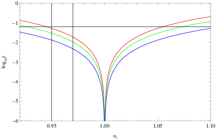
Let us note that for this simple qualitative analysis we assumed that $x$ is constant.

Thus what we demonstrated is that the viable $F(R)$ gravities may be classified mainly into two limiting types of $r-n_{s}$ relations, one identical to the $R^{2}$ model at leading order in $x$, when $x\ll 1$, and one identical to the $\alpha$-attractors $r-n_{s}$ relation, when $x$ takes constant values for a given $F(R)$ gravity. However, we need to note that we did not consider cases for which one of the slow-roll indices may not comply with the slow-roll assumptions, like for instance in the constant-roll case. This would require a different treatment of the study we performed in this letter, since $\ddot{H}\sim H\dot{H}$ in the constant-roll case.

It is noteworthy to state that such a classification among some viable $F(R)$ gravity theories might also be justified by the conformal invariance of the observational indices, so our result is the Jordan frame manifestation of the Einstein frame $\alpha$-attractors result, since the spectral index $n_{s}$ and the tensor-to-scalar ratio $r$ turn out to be nearly the same if calculated in the Jordan or in the Einstein frame Kaiser:1995nv; Domenech:2016yxd; Brooker:2016oqa; Kaiser:1994vs.

Furthermore, most of $F(R)$ gravity approaches use $\dot{\epsilon}_{i}=0$, $i=1,2,3$, for extracting the spectral index of Eq. (9). This however is a severe inconsistency in the formalism of $F(R)$ gravity inflation. Actually this condition used in Ref. Hwang:2005hb, namely $\dot{\epsilon}_{1}=0$, is too strong, since the only thing required for obtaining the spectral index of Eq. (9), is $\dot{\epsilon}_{i}\ll 1$, $i=1,2,3$. We resolved this issue in detail in Ref. Oikonomou:2020krq. This slight change of the condition on the derivatives of the slow-roll indices, and specifically of the slow-roll index $\epsilon_{1}$ from $\dot{\epsilon}_{1}=0$ to $\dot{\epsilon}_{1}\ll 1$, has an impact on $\epsilon_{4}$ and subsequently on the $r-n_{s}$ relation. Moreover it can have some effect on the phenomenology of some $F(R)$ gravities. This issue is quite intriguing, since the condition $\dot{\epsilon}_{1}=0$ would make even viable $F(R)$ gravities to yield non-viable results, as shown in Oikonomou:2020krq where we showed explicitly how the condition $\dot{\epsilon}_{1}=0$ would render even viable $F(R)$ gravities, like the $R^{2}$ model non-viable. In fact, the authors of Ref. Hwang:2005hb derived the expression for the spectral index we quoted in Eq. (9), by using the condition $\dot{\epsilon}_{1}=0$, which is a crucial inconsistency, which we resolved in a mathematical way in Ref. Oikonomou:2020krq. As we showed in Ref. Oikonomou:2020krq, the result of Ref. Hwang:2005hb which we used in Eq. (9) in the present letter, holds true, without the condition $\dot{\epsilon}_{1}=0$. If the condition $\dot{\epsilon}_{1}=0$ is required, then the expression for the spectral index given in Eq. (9) of the present draft would only hold true for power-law gravities $F(R)\sim R^{n}$, for $n\neq 2$, which obviously does not include the $R^{2}$ model. In addition, if the condition $\dot{\epsilon}_{1}=0$ is assumed to hold true, then the $R^{2}$ model would yield an exactly scale invariant power spectrum, see Ref. Oikonomou:2020krq for details. Finally, let us note that the formalism and results which we developed in this work, does not apply in the case that the $F(R)$ gravity model yields $\dot{\epsilon}_{1}=0$, and in effect some power-law $F(R)$ gravities of the form $F(R)=R+\gamma R^{n}$, with $n\neq 2$ cannot be appropriately described by our formalism. We are working along this research lines in order to explain the problem with these theories, strongly related to the slow-roll assumption, and we address this issue in a future work.

This work is supported by MINECO (Spain), FIS2016-76363-P, and by project 2017 SGR247 (AGAUR, Catalonia) (S.D.O).

References

- (1) A. D. Linde, Lect. Notes Phys. 738 (2008) 1 [arXiv:0705.0164 [hep-th]].
- (2) D. S. Gorbunov and V. A. Rubakov, “Introduction to the theory of the early universe: Cosmological perturbations and inflationary theory,” Hackensack, USA: World Scientific (2011) 489 p;
- (3) A. Linde, arXiv:1402.0526 [hep-th];
- (4) D. H. Lyth and A. Riotto, Phys. Rept. 314 (1999) 1 [hep-ph/9807278].
- (5) M. Kamionkowski and E. D. Kovetz, Ann. Rev. Astron. Astrophys. 54 (2016) 227 doi:10.1146/annurev-astro-081915-023433 [arXiv:1510.06042 [astro-ph.CO]].
- (6) S. Nojiri, S. D. Odintsov and V. K. Oikonomou, Phys. Rept. 692 (2017) 1 [arXiv:1705.11098 [gr-qc]].
- (7)
S. Capozziello, M. De Laurentis,
Phys. Rept. 509, 167 (2011);
V. Faraoni and S. Capozziello, The landscape beyond Einstein gravity, in Beyond Einstein Gravity 828 (Springer, Dordrecht, 2010), Vol. 170, pp.59-106. - (8) S. Nojiri, S.D. Odintsov, Phys. Rept. 505, 59 (2011);
- (9) A. de la Cruz-Dombriz and D. Saez-Gomez, Entropy 14 (2012) 1717 [arXiv:1207.2663 [gr-qc]].
- (10) S. D. Odintsov and V. K. Oikonomou, Phys. Rev. D 96 (2017) no.10, 104049 doi:10.1103/PhysRevD.96.104049 [arXiv:1711.02230 [gr-qc]].
- (11) S. Bahamonde, C. G. Bohmer, S. Carloni, E. J. Copeland, W. Fang and N. Tamanini, Phys. Rept. 775-777 (2018) 1 doi:10.1016/j.physrep.2018.09.001 [arXiv:1712.03107 [gr-qc]].
- (12) R. Kallosh and A. Linde, JCAP 1307 (2013) 002 [arXiv:1306.5220 [hep-th]].
- (13) S. Ferrara, R. Kallosh, A. Linde and M. Porrati, Phys. Rev. D 88 (2013) no.8, 085038 [arXiv:1307.7696 [hep-th]].
- (14) R. Kallosh, A. Linde and D. Roest, JHEP 1311 (2013) 198 [arXiv:1311.0472 [hep-th]].
- (15) M. Galante, R. Kallosh, A. Linde and D. Roest, Phys. Rev. Lett. 114 (2015) no.14, 141302 [arXiv:1412.3797 [hep-th]].
- (16) S. Cecotti and R. Kallosh, JHEP 1405 (2014) 114 [arXiv:1403.2932 [hep-th]].
- (17) J. J. M. Carrasco, R. Kallosh and A. Linde, JHEP 1510 (2015) 147 [arXiv:1506.01708 [hep-th]].
- (18) A. Linde, JCAP 1505 (2015) 003 doi:10.1088/1475-7516/2015/05/003 [arXiv:1504.00663 [hep-th]].
- (19) D. Roest and M. Scalisi, Phys. Rev. D 92 (2015) 043525 doi:10.1103/PhysRevD.92.043525 [arXiv:1503.07909 [hep-th]].
- (20) R. Kallosh, A. Linde and D. Roest, JHEP 1408 (2014) 052 doi:10.1007/JHEP08(2014)052 [arXiv:1405.3646 [hep-th]].
- (21) J. Ellis, D. V. Nanopoulos and K. A. Olive, JCAP 1310 (2013) 009 [arXiv:1307.3537 [hep-th]].
- (22) Y. F. Cai, J. O. Gong and S. Pi, Phys. Lett. B 738 (2014) 20 doi:10.1016/j.physletb.2014.09.009 [arXiv:1404.2560 [hep-th]].
- (23) Z. Yi and Y. Gong, arXiv:1608.05922 [gr-qc].
- (24) S. D. Odintsov and V. K. Oikonomou, Phys. Rev. D 94 (2016) no.12, 124026 doi:10.1103/PhysRevD.94.124026 [arXiv:1612.01126 [gr-qc]].
- (25) E. Elizalde, S. D. Odintsov, E. O. Pozdeeva and S. Y. Vernov, JCAP 1602 (2016) no.02, 025 [arXiv:1509.08817 [gr-qc]].
- (26) C. P. Burgess, M. Cicoli, S. de Alwis and F. Quevedo, JCAP 1605 (2016) 032 doi:10.1088/1475-7516/2016/05/032 [arXiv:1603.06789 [hep-th]].
- (27) A. A. Starobinsky, Phys. Lett. 91B (1980) 99 [Adv. Ser. Astrophys. Cosmol. 3 (1987) 130]. doi:10.1016/0370-2693(80)90670-X
- (28) F. L. Bezrukov and M. Shaposhnikov, Phys. Lett. B 659 (2008) 703 doi:10.1016/j.physletb.2007.11.072 [arXiv:0710.3755 [hep-th]].
- (29) J. c. Hwang and H. Noh, Phys. Rev. D 71 (2005) 063536 doi:10.1103/PhysRevD.71.063536 [gr-qc/0412126].
- (30) V. Oikonomou, “Rectifying an Inconsistency in Gravity Inflation,” European Physics Letters in press, [arXiv:2004.10778 [gr-qc]].
- (31) Y. Akrami et al. [Planck Collaboration], arXiv:1807.06211 [astro-ph.CO].
- (32) R. Kallosh, A. Linde and A. Westphal, Phys. Rev. D 90 (2014) no.2, 023534 doi:10.1103/PhysRevD.90.023534 [arXiv:1405.0270 [hep-th]].; A. D. Linde, Phys. Lett. B 129 (1983) 177. doi:10.1016/0370-2693(83)90837-7
- (33) S. Ferrara, R. Kallosh and A. Linde, JHEP 1410 (2014) 143 doi:10.1007/JHEP10(2014)143 [arXiv:1408.4096 [hep-th]].
- (34) D. I. Kaiser, [astro-ph/9507048].
- (35) G. Domenech and M. Sasaki, Int. J. Mod. Phys. D 25 (2016) no.13, 1645006 [arXiv:1602.06332 [gr-qc]].
- (36) D. J. Brooker, S. D. Odintsov and R. P. Woodard, Nucl. Phys. B 911 (2016) 318 [arXiv:1606.05879 [gr-qc]].
- (37) D. I. Kaiser, Phys. Rev. D 52 (1995) 4295 [astro-ph/9408044].