Light-by-light scattering sum rule for radiative transitions of bottomonia

Several model-independent sum rules were derived for the forward light-by-light scattering, and were exactly verified at leading order in scalar and spinor QED Gerasimov 1966; Drell and Hearn 1966; Drechsel and Tiator 2004; Pascalutsa and Vanderhaeghen 2010; Pascalutsa et al. 2012. Such sum rules are valid for the case when at least one photon is real and the other is spacelike or below the first particle production threshold, i.e., for photon virtualities $q_{1}^{2}\leq s_{0}$, $q_{2}^{2}=0$, where $s_{0}$ is the particle production threshold. Three of these sum rules have the form of a superconvergence relation, for which an integral over an experimentally measurable quantity yields zero Pascalutsa et al. 2012. One of these is a helicity sum rule of the form

where $\sigma_{0}$ and $\sigma_{2}$ are the total helicity cross sections for the $\gamma^{\ast}\gamma\to X$ processes for total helicity 0 and 2, respectively, where $X$ denotes the sum over all allowed final states. Such light-by-light sum rules have been applied within different field theories in both perturbative and nonperturbative settings Pascalutsa and Vanderhaeghen 2010; Pascalutsa et al. 2012; Pauk et al. 2013. Furthermore, their application to the $\gamma^{\ast}\gamma$ production of light-quark mesons has been discussed in Refs. Pascalutsa et al. 2012; Danilkin and Vanderhaeghen 2017a, and the application to the $\gamma\gamma$ production of charmonium states was discussed in Ref. Danilkin and Vanderhaeghen 2017b. For the pseudoscalar, scalar, axial-vector, and tensor mesons, where $\gamma^{\ast}\gamma\to X$ data are available, these sum rules were verified within 10% - 30% experimental accuracy Danilkin and Vanderhaeghen 2017a.

In the present work we investigate the extension of such sum rules, when one of the virtual photons is replaced by a vector quarkonium state. For the conventional heavy-quark $Q\bar{Q}$ bound states, radiative transitions have been measured quite extensively in the past decades by collaborations at the charm and $B$ factories, CLEO@CESR, BABAR@PEP-II, Belle@KEKB, and BESIII@BEPCII, and will be studied in the near future by Belle-II.

The study of light-by-light sum rules in the heavy quarkonium sector may also be worthwhile in light of the plethora of new states, so-called $XYZ$ states, which have been found in recent years above open heavy flavor thresholds at all of these facilities, see e.g. Refs. Chen et al. 2016; Lebed et al. 2017; Olsen et al. 2018 for some recent reviews and references therein. Such sum rule relations have the potential to reveal how much of the radiative decay strength from or into vector quarkonium states results from possible exotic mesons. An example is the $X(3872)$ state with $J^{PC}=1^{++}$, which sits right at the $D\bar{D}^{\ast}$ threshold, for which the radiative transitions $\gamma J/\psi$ and $\gamma\psi^{\prime}$ have been proposed as a diagnostic tool for studying the nature of this state Swanson 2004, shedding light on its hybrid charmonium-molecular nature. Rare decays of $X(3872)$ will be an important part of the PANDA Lutz et al. 2009 scientific program where such studies are feasible even at the start of data taking. Also, at BESIII the first radiative transition between two exotic mesons has been observed in the process $Y(4260)\to\gamma X(3872)$ Ablikim et al. 2014, and detailed studies of radiative transitions can be expected from Belle-II in the near future Altmannshofer et al. 2019.

The outline of this work is as follows. In Section II, we introduce the helicity sum rule that we will study in this work for radiative transitions between quarkonium states, of which one has $J^{PC}=1^{--}$ quantum numbers. In Section III we describe the potential model adopted from Refs. Deng et al. 2017a; Deng et al. 2017b to reproduce heavy quarkonium wave functions. In Section IV we review the formalism to evaluate the leading radiative transitions between quarkonium states with defined total helicity, and make a comparison between available experimental values and theoretical results in the literature. In Section V we make use of experimental information on the radiative transitions $\Upsilon(mS)\to\gamma\chi_{bJ}(nP)$ for $m>n$, as well as theoretical estimates for $\chi_{bJ}(nP)\to\gamma\Upsilon(mS)$ for $n\geq m$, and evaluate the derived helicity sum rule. We provide a quantitative discussion for the $\Upsilon(1S)$, $\Upsilon(2S)$, and $\Upsilon(3S)$ states. Finally, a summary and outlook is given in Section VI.

In the case when one photon in Eq. (1) is replaced by a vector quarkonium state, one needs to take into account its nonpointlike structure. In full analogy to the original Gerasimov-Drell-Hearn sum rule Gerasimov 1966; Drell and Hearn 1966; Drechsel and Tiator 2004, it gives the relation to the anomalous magnetic moment $a_{V}$. Therefore, for the states below the $B\bar{B}$ threshold ($m_{V}^{2}<4\,m_{B}^{2}$) it holds that

where we expressed the helicity cross sections in Eq.(1) in terms of the $\gamma V\to\gamma V$ helicity amplitudes $M_{\lambda_{\gamma}^{\prime}\lambda_{V}^{\prime},\lambda_{\gamma}\lambda_{V}}$. The integral in Eq.(2) extends over both bound states and open-flavor states. In principle, all neutral intermediate quarkonium states with even C parity can contribute to this sum rule, see Fig. 1. These are not only scalar $J^{PC}=0^{++}$, pseudoscalar $0^{-+}$, axial-vector $1^{++}$, and tensor $2^{++}$ mesons, but also quarkonium states that can carry exotic quantum numbers, such as e.g. $1^{-+}$ and $2^{-+}$. In our analysis, we limit ourselves to the states that correspond to conventional quantum numbers and that are expected to be dominant ones below the $B\bar{B}$ threshold. Furthermore, all of the transitions to pseudoscalar $0^{-+}$ mesons corresponding with magnetic dipole transitions (M1) turn out to be strongly suppressed for the bottomonium transitions, as compared to the transitions to $0^{++},1^{++},2^{++},...$, which correspond predominantly to electric dipole transitions (E1), as discussed below. For bottomonia the anomalous magnetic moment is a small quantity and has been estimated as Brambilla et al. 2011

Using such value, the sum rule of Eq. (2) should yield almost zero for bottomonia, i.e., SR $\sim 8\,\text{nb}$.

Unitarity allows us to relate the imaginary part of the $\gamma V\to\gamma V$ helicity amplitude $M_{\lambda_{\gamma}^{\prime}\lambda_{V}^{\prime},\lambda_{\gamma}\lambda_{V}}$ to the $X\to\gamma V$ (for $m_{X}>m_{V}$) or $V\to\gamma X$ (for $m_{V}>m_{X}$) transition amplitudes ${\cal M}_{\Lambda,\lambda_{\gamma}\lambda_{V}}$

where $\Lambda=\lambda_{\gamma}-\lambda_{V}$ denotes the helicity of the quarkonium state $X$, with $\lambda_{V}$ ($\lambda_{\gamma}$) being the helicity of the vector quarkonium state $V$ (photon). In the narrow-resonance approximation, Eq. (II) can be written as

which allows us to rewrite the sum rule (2) in terms of the helicity-dependent radiative widths $\Gamma_{\Lambda=0,2}$ for either the $X\to\gamma V$ or $V\to\gamma X$ transitions. For the $X\to\gamma V$ transitions, the helicity radiative widths are given by:

where the photon energy is given by $k=(m_{X}^{2}-m_{V}^{2})/(2m_{X})$ and $\Gamma^{\rm{EM}}(X)$ is the unpolarized radiative width of the corresponding transition. The corresponding expressions for the helicity radiative widths for the $V\to\gamma X$ transitions are obtained from expressions analogous to Eq. (6) with the replacement $X\leftrightarrow V$.

Substituting Eqs. (II) and (6) into the sum rule (2) yields the master formula that we will use in this work:

where we neglected the term proportional to $a_{V}^{2}$ as well as the continuum contribution from the open-flavor channels. The latter was estimated using the quark-hadron duality argument Novikov et al. 1978 in total analogy to Pascalutsa et al. 2012; Danilkin and Vanderhaeghen 2017b. It gives a negligible contribution in the range of $\sim 0.3-7.3$ nb, depending on $V=\Upsilon(1S),\Upsilon(2S),\Upsilon(3S)$. Furthermore, in Eq. (II) we introduced the helicity ratios

which (as will be shown below) are universal constants in the case of E1 transitions, and depend only on the total angular momentum of the state $X$.

Since the relativistic effects in bottomonia are expected to be small, the spectrum and wave functions can be calculated with the help of the Schrödinger equation and a conventional heavy quarkonium potential,

where the Cornell potential $V_{0}$ is the sum of one-gluon exchange ($V_{V}$) and linear scalar confining ($V_{S}$) parts Eichten et al. 1978,

while $V_{SD}$ is a spin-dependent part which splits into the spin-spin ($V_{SS}$), spin-orbit ($V_{LS}$), and tensor ($V_{T}$) potentials. Up to order $1/m_{b}^{2}$, they are given by

where $\vec{L}$ is the relative orbital momentum operator and $\vec{S}=\vec{s}_{1}+\vec{s}_{2}$ is the total spin operator of the quark-antiquark system. Typically, the spin-dependent terms are treated using the leading-order perturbation theory. However, in the present work we follow Deng et al. Deng et al. 2017a; Deng et al. 2017b and account for them nonperturbatively. In order to do that, several modifications are needed.

First of all, one needs to take the matrix elements over operators in the $|L,S,J,j\rangle$ basis (where $j$ is the spin projection of $J$ on a fixed axis)

and regularize a $1/r^{3}$ behavior in the terms $V_{LS}$ and $V_{T}$ when $r\rightarrow 0$. The most obvious way to do this is to saturate these potentials at some low-distance scale $r_{C}$, i.e., set $V_{T}(r)=V_{T}(r_{c})$ and $V_{LC}(r)=V_{LV}(r_{c})$ when $r<r_{C}$ Deng et al. 2017b.

Second, the physical hyperfine interaction corresponds to a smeared $\delta$ function Barnes et al. 2005,

where $1/\sigma$ is a radius of order $\propto 1/m_{b}$.

Finally, in order to effectively account for the creation of virtual light $q\bar{q}$ pairs in the Wilson loop, one considers a screening of the confining potential at large distances $r\gg 1/\mu$:

The unknown parameters were determined in Ref. Deng et al. 2017b by fitting the spectrum. A fairly good description of the energy levels was achieved with the following choice of parameters:

In our work we were able to reproduce the results of Ref. Deng et al. 2017b to an accuracy of less than $1$ MeV in the energy levels and use these results for the masses of the yet unmeasured $\chi_{b0}(3P)$ and $\chi_{b2}(3P)$ states, as well as to evaluate the radiative transition matrix elements.

The helicity amplitudes entering Eq. (6) can be expressed, choosing the Coulomb gauge, as

with the definition $\Lambda\equiv\lambda_{\gamma}-\lambda_{V}$, where $\vec{J}(\vec{x})$ is the electromagnetic current operator, and where we introduced the labels $i$ (initial) and $f$ (final) instead of $X$ and $V$ to keep further calculations independent of the direction of the transition. Here the initial and final internal states are labeled by $|\psi_{i}\rangle=|n_{i}L_{i}S_{i}J_{i}j_{i}\rangle$ and $|\psi_{f}\rangle=|n_{f}L_{f}S_{f}J_{f}j_{f}\rangle$, where $j_{i},j_{f}$ are the spin projections on a fixed axis. By going to the rest frame of the decaying state, we can orient the quantization axis along the photon momentum direction $\vec{k}$ and identify the spin projections in terms of helicities, e.g., for the $X\to\gamma V$ transitions, as $j_{i}=\Lambda$, $j_{f}=-\lambda_{V}$. Note that in the matrix element of Eq. (16) we use the covariant normalization for the electromagnetic field, but initial and final quarkonium states are normalized nonrelativistically.

A multipole expansion of the electromagnetic field allows to express the matrix element of Eq. (16) as

where $j_{L}(k|\vec{x}|)$ denote the spherical Bessel functions, and $\vec{Y}^{M_{J}}_{LJ}(\hat{x})$ is the vector spherical harmonic function, defined in terms of the product of spherical harmonics $Y_{LM_{L}}(\hat{x})$ with the photon polarization vector $\vec{\varepsilon}_{\lambda}$ as

Furthermore, in Eq. (17) the first term, proportional to the squared bracket, corresponds to the electric multipole transitions, whereas the last term corresponds to the magnetic multipole transitions.

The long-wavelength limit is governed by $kr\ll 1$, where $r=|\vec{x}|$ is the size of the bottomonium system. Because $j_{L}(kr)\sim(kr)^{L}$ in this limit, the helicity amplitude in Eq. (17) will be dominated by the lowest multipoles. Out of these multipoles, the dominant one corresponds to the electric dipole (E1) radiative transitions, i.e., for $J=1$, due to the behavior of the $j_{0}(kr)$ term. The magnetic dipole transition (M1) as well as higher multipoles are all suppressed by extra powers of $(kr)$. For the sum rule tests for the bottomonium system considered in this paper, where we envisage a numerical precision in the $5-10\%$ range, we can therefore use the nonrelativistic electromagnetic current operator $\vec{J}(\vec{x})$ as

where $m_{Q}=m_{\bar{Q}}=m_{b}$, $e_{Q}=-e_{\bar{Q}}=-1/3\,e$ is the bottom quark charge, $\vec{r}$ is the relative vector between quark and antiquark positions, and ${\hat{\vec{p}}}_{Q}$ and ${\hat{\vec{p}}}_{\bar{Q}}$ are the momentum operators for the quark and anti-quark, respectively. This yields the $E1$ matrix element from Eq. (17):

where $\hat{\vec{p}}=({\hat{\vec{p}}}_{Q}-{\hat{\vec{p}}}_{\bar{Q}})/2$ is the relative momentum operator in the quarkonium system.

Furthermore, to describe the E1 radiative transitions for the bottomonium states with $n_{i}=n_{f}$ (and to a lesser extent transitions of nearby $n_{i}$ and $n_{f}$), the long-wavelength limit provides a rather good approximation. As will be shown below, these transitions give the dominant contributions to the sum rule. In this limit the matrix element of Eq. (20) is given by

where we used the Ehrenfest theorem in the transition from the first to the second line. In result, the nonrelativistic (NRel) expression for the E1 radiative transition width is given by

where the mass difference $m_{i}-m_{f}$ was approximated by the photon energy $k$.

As we will only consider transitions from $L_{i}=1\to L_{f}=0$ or $L_{i}=0\to L_{f}=1$ spin-triplet states ($S_{i}=S_{f}=1$) in the following, Eq. (22) reduces to:

where $R_{i}$ and $R_{f}$ denote the radial wave functions of initial and final states. Note that, for the actual calculations, we account for finite-size corrections to the nonrelativistic E1 result by the replacement Novikov et al. 1978

which are practically only important for the subdominant contributions to the sum rule.

A more systematic inclusion of relativistic effects in calculating the E1 decay widths of heavy quarkonia requires estimating the relativistic corrections to the wave functions, in addition to the recoil and finite-size effects. Such early estimates of the relativistic corrections to the heavy quarkonium E1 decay rates in an expansion up to order $v^{2}/c^{2}$ were performed using different potential models, including a Richardson type of potential Moxhay and Rosner 1983, a Coulomb-plus-linear Cornell type potential for $r\gtrsim 0.1$ fm, modified to saturate for $r\lesssim 0.1$ fm McClary and Byers 1983, and a Buchmüller-Tye potential with a scalar confining part Grotch et al. 1984. To compare the first-order relativistic corrections between different approaches, we express the relativistic (Rel) calculations of the E1 decay widths of bottomonia as

In Table 1 we compare the relativistic correction factor $\delta$ for the $\chi_{bJ}(1P)\to\gamma\Upsilon(1S)$ and $\chi_{bJ}(2P)\to\gamma\Upsilon(2S)$ decays in the three above-mentioned calculations. For the decays shown in Table 1, the bulk of the relativistic corrections comes from the relativistic modifications to the wave functions, and obviously depends on the choice of the potential. For example, for the $\chi_{bJ}(1P)\to\gamma\Upsilon(1S)$ decay rates, Refs. Moxhay and Rosner 1983; McClary and Byers 1983 found corrections of order $\delta\sim+10\%$, whereas Ref. Grotch et al. 1984 reported corrections of order $\delta\sim-20\%$ to $-15\%$ for the same transitions.

In view of the expected corrections in the $10-20~\%$ range for the lower bottomonium states, our strategy in minimizing the model uncertainties in the sum rule estimates is to use the experimental values of the E1 decay widths wherever possible. The latter are available for the $\Upsilon(2S)\to\gamma\chi_{bJ}(1P)$, $\Upsilon(3S)\to\gamma\chi_{bJ}(2P)$, and $\Upsilon(3S)\to\gamma\chi_{bJ}(1P)$ transitions. For the $\chi_{bJ}(nP)\to\gamma\Upsilon(nS)$ transitions (for $n=1,2,3$), for which the absolute E1 decay widths are not known empirically at present, we will compare their calculated values between five different realistic models that are fit to the spectrum. The spread in the $\Gamma^{\rm{E1}}$ model predictions will be taken as an estimate of the error on the E1 decay width.

To evaluate the sum rule (II), besides the unpolarized radiative width, we also need the helicity ratios $r_{\Lambda=0,2}(X)$. We will work in the E1 approximation, i.e. neglect the M2 transition for $\chi_{b1}(n_{i}P)\to\Upsilon(n_{f}S)$ and the M2 and E3 transitions for $\chi_{b2}(n_{i}P)\to\Upsilon(n_{f}S)$. In the E1 approximation, the coefficients $r_{\Lambda}(X)$ can be expressed as ratios of Clebsch-Gordan coefficients and do not depend on the internal structure of the mesons. Their values are shown in Table 2.

Note that in the extreme nonrelativistic limit where the fine structure is neglected, i.e. when the three $\chi_{bJ}(nP)$ states (for $J=0,1,2$) are degenerate, the corresponding helicity radiative widths all become proportional to the same E1 squared matrix element. As a consequence, the helicity-0 and helicity-2 sum rule contributions of the three $\chi_{bJ}(nP)$ states are given by

which shows that in this extreme limit the sum rule holds exactly for the radiative transitions originating from each shell separately. When calculating with realistic potentials below, where the degeneracy between the three $\chi_{bJ}(nP)$ states is lifted, we will nevertheless observe an approximate cancellation between these states. However, the sum rule of Eq. (II) in general only holds when summing over all radiative transitions to or from a given $\Upsilon(nS)$ state.

The central objects in the evaluation of the sum rule of Eq. (II) are the radiative transitions of either $X\to V\gamma$ or $V\to\gamma X$. Several of these transitions have been studied by the Crystal Ball, ARGUS, CLEO, BABAR, and Belle collaborations, as summarized by the Particle Data Group (PDG) Tanabashi et al. 2018. Absolute radiative widths are known for the transitions of $\Upsilon(mS)\to\gamma\chi_{bJ}(nP)$ states when $m>n$, and are given in Tables 3 and 4. For the opposite transitions of $\chi_{bJ}(nP)\to\gamma\Upsilon(mS)$ when $n\geq m$ only branching fractions Br$(\chi_{bJ}(nP)\to\gamma\Upsilon(mS))$ have been measured. In the absence of the total widths these results cannot be converted into partial widths. For these transitions we will use the results of the potential model, based on Ref. Deng et al. 2017b, and outlined in Sections III and IV. To account for the theory uncertainty in the E1 radiative transitions, we include the spread between different theory predictions as our error estimate on this quantity. For the nonrelativistic models, we include the predictions from Refs. Barnes et al. 2005; Li and Chao 2009; Segovia et al. 2016, which mainly differ in the form of the potential. The result of Ref. Li and Chao 2009 corresponds to the first-order relativistically corrected wave function with a screened potential model. As for the relativized quark model, we refer to Refs. Barnes et al. 2005; Godfrey and Moats 2015 where the spinless Salpeter equation was solved, and to Ref. Ebert et al. 2003 which relied on the relativized quasipotential approach.

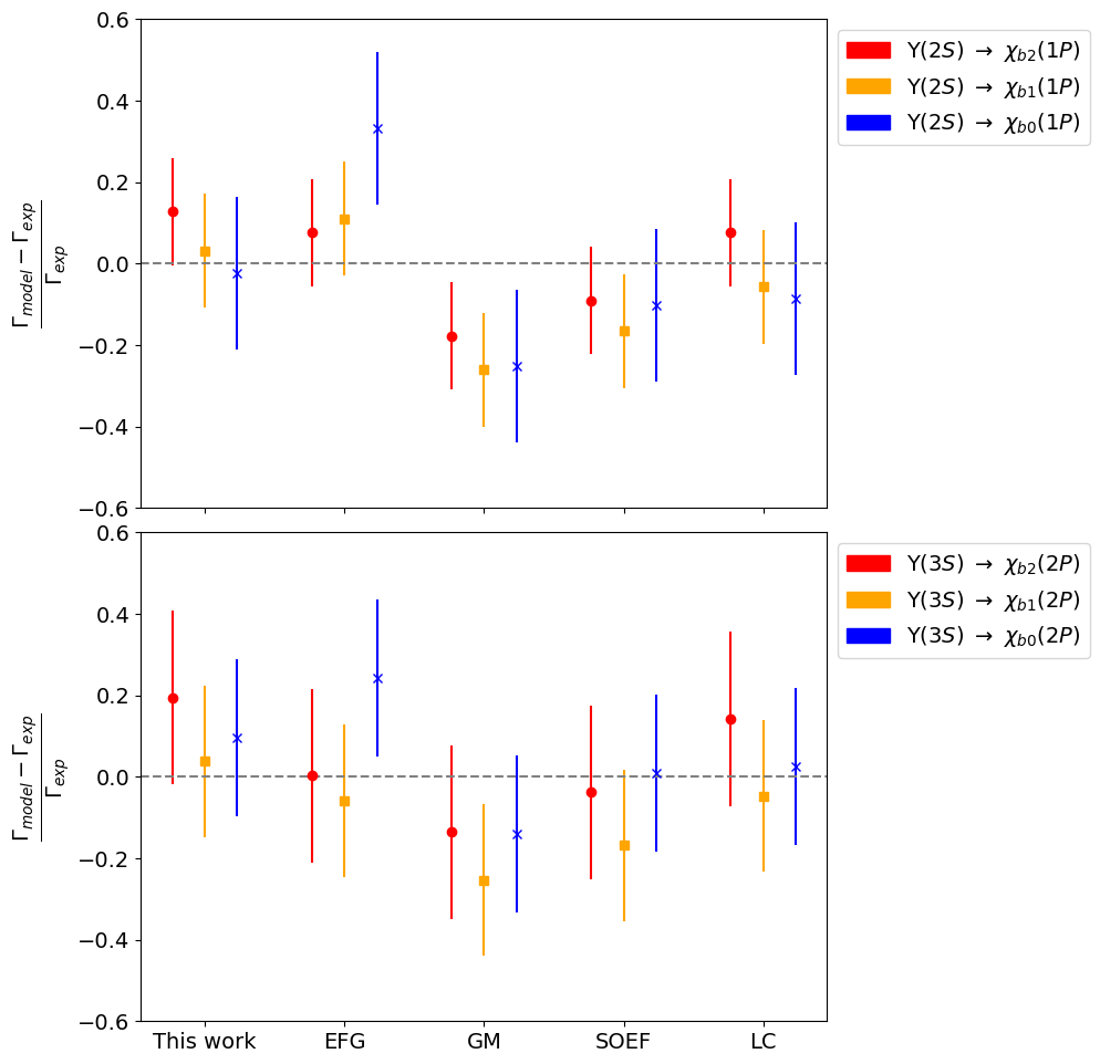
We start by comparing the theoretical E1 radiative widths for the $\Upsilon(2S)\to\gamma\,\chi_{bJ}(1P)$ and $\Upsilon(3S)\to\gamma\,\chi_{bJ}(2P)$ transitions with their experimental results in Tables 3 and 4, respectively. We see that for nearly all of these transitions the central values (calculated as explained in Sections III and IV) agree with experiment to within 15%. The spread between the different theoretical values is also in this range, as is illustrated in Fig. 2. We therefore feel confident that we can estimate the unknown radiative widths $\chi_{bJ}(nP)\to\gamma\Upsilon(mS)$, for $m=1,2,3$, with an accuracy at the 20% level or better.

References

- Gerasimov (1966) S. B. Gerasimov, Sov. J. Nucl. Phys. 2, 430 (1966), [Yad. Fiz.2,598(1965)]
- Drell and Hearn (1966) S. Drell and A. C. Hearn, Phys. Rev. Lett. 16, 908 (1966)
- Drechsel and Tiator (2004) D. Drechsel and L. Tiator, Ann. Rev. Nucl. Part. Sci. 54, 69 (2004)
- Pascalutsa and Vanderhaeghen (2010) V. Pascalutsa and M. Vanderhaeghen, Phys. Rev. Lett. 105, 201603 (2010)
- Pascalutsa et al. (2012) V. Pascalutsa, V. Pauk, and M. Vanderhaeghen, Phys. Rev. D 85, 116001 (2012)
- Pauk et al. (2013) V. Pauk, V. Pascalutsa, and M. Vanderhaeghen, Phys. Lett. B725, 504 (2013)
- Danilkin and Vanderhaeghen (2017a) I. Danilkin and M. Vanderhaeghen, Phys. Rev. D95, 014019 (2017a)
- Danilkin and Vanderhaeghen (2017b) I. Danilkin and M. Vanderhaeghen, Phys. Rev. D 96, 056003 (2017b)
- Chen et al. (2016) H.-X. Chen, W. Chen, X. Liu, and S.-L. Zhu, Phys. Rept. 639, 1 (2016)
- Lebed et al. (2017) R. F. Lebed, R. E. Mitchell, and E. S. Swanson, Prog. Part. Nucl. Phys. 93, 143 (2017)
- Olsen et al. (2018) S. L. Olsen, T. Skwarnicki, and D. Zieminska, Rev. Mod. Phys. 90, 015003 (2018), eprint 1708.04012
- Swanson (2004) E. S. Swanson, Phys. Lett. B 598, 197 (2004)
- Lutz et al. (2009) M. Lutz et al. (PANDA) (2009), eprint 0903.3905
- Ablikim et al. (2014) M. Ablikim et al. (BESIII), Phys. Rev. Lett. 112, 092001 (2014)
- Altmannshofer et al. (2019) W. Altmannshofer et al. (Belle-II), PTEP 2019, 123C01 (2019), [Erratum: PTEP 2020, 029201 (2020)], eprint 1808.10567
- Deng et al. (2017a) W.-J. Deng, H. Liu, L.-C. Gui, and X.-H. Zhong, Phys. Rev. D 95, 034026 (2017a)
- Deng et al. (2017b) W.-J. Deng, H. Liu, L.-C. Gui, and X.-H. Zhong, Phys. Rev. D 95, 074002 (2017b)
- Brambilla et al. (2011) N. Brambilla et al., Eur. Phys. J. C 71, 1534 (2011)
- Novikov et al. (1978) V. A. Novikov, L. B. Okun, M. A. Shifman, A. I. Vainshtein, M. B. Voloshin, and V. I. Zakharov, Phys. Rept. 41, 1 (1978)
- Eichten et al. (1978) E. Eichten, K. Gottfried, T. Kinoshita, K. Lane, and T.-M. Yan, Phys. Rev. D 17, 3090 (1978), [Erratum: Phys.Rev.D 21, 313 (1980)]
- Barnes et al. (2005) T. Barnes, S. Godfrey, and E. S. Swanson, Phys. Rev. D72, 054026 (2005)
- Moxhay and Rosner (1983) P. Moxhay and J. L. Rosner, Phys. Rev. D28, 1132 (1983)
- McClary and Byers (1983) R. McClary and N. Byers, Phys. Rev. D28, 1692 (1983)
- Grotch et al. (1984) H. Grotch, D. A. Owen, and K. J. Sebastian, Phys. Rev. D30, 1924 (1984)
- Tanabashi et al. (2018) M. Tanabashi et al. (Particle Data Group), Phys. Rev. D 98, 030001 (2018)
- Li and Chao (2009) B.-Q. Li and K.-T. Chao, Commun. Theor. Phys. 52, 653 (2009)
- Segovia et al. (2016) J. Segovia, P. G. Ortega, D. R. Entem, and F. Fernandez, Phys. Rev. D93, 074027 (2016)
- Godfrey and Moats (2015) S. Godfrey and K. Moats, Phys. Rev. D92, 054034 (2015)
- Ebert et al. (2003) D. Ebert, R. N. Faustov, and V. O. Galkin, Phys. Rev. D67, 014027 (2003)
- Aubert et al. (2006) B. Aubert et al. (BaBar), Phys. Rev. D 74, 071101 (2006)
- Bhardwaj et al. (2011) V. Bhardwaj et al. (Belle), Phys. Rev. Lett. 107, 091803 (2011)
- Aubert et al. (2009) B. Aubert et al. (BaBar), Phys. Rev. Lett. 102, 132001 (2009)
- Aaij et al. (2014) R. Aaij et al. (LHCb), Nucl. Phys. B 886, 665 (2014)