Strong zero modes from geometric chirality in quasi-one-dimensional Mott insulators

Quantum many-body systems supporting local degrees of freedom that remain coherent for long times even away from the ground state may open up nonzero temperature, or even non-equilibrium, regimes for quantum information processing Fendley 2012; Fendley 2014; Fendley 2016; Alicea and Fendley 2016; Kemp et al. 2017; Else et al. 2017; Kemp et al.; Yates et al.; Wootton and Pachos 2011; Stark et al. 2011; Bauer and Nayak 2013; Huse et al. 2013; Parameswaran et al. 2017; Alet and Laflorencie 2018; Parameswaran and Vasseur 2018; Abanin et al. 2019; Wahl and Béri. A key requirement for such coherence is the presence of degeneracies across the energy spectrum. “Strong zero modes” Fendley 2016 provide a compelling mechanism for this (another route is by many-body localization Wootton and Pachos 2011; Stark et al. 2011; Bauer and Nayak 2013; Huse et al. 2013; Parameswaran et al. 2017; Alet and Laflorencie 2018; Parameswaran and Vasseur 2018; Abanin et al. 2019; Wahl and Béri): these are objects that commute with the Hamiltonian (up to corrections exponentially decaying in system size), but they do not commute with a discrete symmetry, hence ensuring spectral degeneracies. When located at the system edge, they furthermore furnish the desired long-time-coherent local degrees of freedom Fendley 2012; Fendley 2014; Fendley 2016; Alicea and Fendley 2016; Kemp et al. 2017; Else et al. 2017; Kemp et al.; Yates et al..

One of the most intriguing paradigms where zero modes appear are quantum clock models with $\mathbb{Z}_{n\geq 3}$ symmetry Fendley 2012; Fendley 2014; Fendley 2016; Alicea and Fendley 2016. The zero modes include $\mathbb{Z}_{n}$-parafermions, signifying a (nonlocal) relation to electronic systems proposed for beyond–Majorana schemes of topological quantum computation Lindner et al. 2012; Cheng 2012; Clarke et al. 2013; Mong et al. 2014; Tsvelik 2014; Klinovaja and Loss 2014; Zhang and Kane 2014; Orth et al. 2015; Alexandradinata et al. 2016; Alavirad et al. 2017; Calzona et al. 2018; Mazza et al. 2018; Fendley 2012; Fendley 2014; Fendley 2016; Hutter and Loss 2016; Alicea and Stern 2015; Alicea and Fendley 2016; Chew et al. 2018; Santos et al. 2019. To support strong zero modes, the clock models require a chiral (i.e., reflection-symmetry breaking) deformation of their couplings Fendley 2012; Fendley 2014; Fendley 2016; Alicea and Fendley 2016; Jermyn et al. 2014; Zhuang et al. 2015; Moran et al. 2017. While phase transitions in the chiral quantum clock model universality class have seen realizations Fendley et al. 2004; Lecheminant and Nonne 2012; Tsvelik and Kuklov 2012; Samajdar et al. 2018; Keesling et al. 2019, the chiral quantum clock models themselves, and their strong zero modes, are yet to find their origin in an underlying microscopic system.

Here we describe a paradigm for how chiral quantum clock models and their strong zero modes can arise in Mott insulators. While somewhat abstract in terms of clock models, chirality is a simple geometrical feature for particles hopping on a lattice Buda et al. 1992, with examples such as chiral nanotubes, molecules, or crystals Saito et al. 1998; Fasman 2013. Our approach is centered on the combination of such geometric chirality with strong interactions.

We focus on the simplest case of $\mathbb{Z}_{3}$ symmetry and study spinless fermion systems such as the three-leg ladder in Fig. 1. We take two complementary approaches: (i) bosonization that captures generic features beyond a single microscopic model but which is only phenomenological in interactions, and (ii) strong-interaction perturbation theory for the system in Fig. 1. Using bosonization, we show how chiral-quantum-clock-model physics, including zero modes, can arise in the presence of certain symmetries (e.g., $\mathbb{Z}_{3}$ and time-reversal) and sufficiently strong and chiral interactions. In our lattice system, we provide an explicit mapping to the chiral three-state clock model perturbed by terms arising via superexchange, and assess the presence of strong zero modes by computing dynamical correlators of clock operators at the edge using exact diagonalization.

Models and symmetries.- We set our terminology using the system in Fig. 1. Anticipating the clock-model mapping, we refer to the positions $i$ along the legs as sites. The legs are of length $\ell$ and the sites are $a_{0}$ apart. The Hamiltonian is $H=H_{0}+H_{\text{int}}$ with

Here $c^{\dagger}_{i,a+3}=c^{\dagger}_{i,a}$ creates a fermion at site $i$ and leg $a\in\{0,1,2\}$; $n_{i,a}=c_{i,a}^{\dagger}c_{i,a}$ is the corresponding number operator. We use real intraleg and interleg tunneling amplitudes, $J$ and $J_{\perp}$, respectively.

Geometric chirality is present if $V_{1}\neq V_{2}$. We characterize this by introducing $V=\frac{1}{3}\sum_{a}V_{a}$ and

The system is invariant under the $\mathbb{Z}_{3}$ transformation $\mathcal{S}$ cyclically permuting the legs. Further symmetries include time-reversal $\mathcal{T}$ and, for the bulk physics (i.e., far from the boundaries), lattice translations along the legs. The generic systems we shall discuss are three-leg ladders beyond Eq. (Strong zero modes from geometric chirality in quasi-one-dimensional Mott insulators), but which still respect these symmetries sym. We work at $1/3$ filling, $\sum_{i,a}n_{i,a}a_{0}/\ell=1$.

Low-energy processes.- We next prepare for bosonization by describing the low-energy bulk processes. By low-energy, we mean processes near the Fermi points. Our bosonization thus starts with moderate interactions; however, its phenomenological scope is broader and includes strong interactions Giamarchi 2003; Gogolin et al. 2004. We first diagonalize the $\mathbb{Z}_{3}$ transformation using $f_{i,\alpha}=\sum_{a}v_{\alpha a}c_{i,a}$, where $v$ is a $3\times 3$ unitary matrix; this diagonalizes the single-particle Hamiltonian into three bands labeled by $\alpha\in\{1,2,3\}$ (Fig. 2 for our concrete model kFf). $\mathbb{Z}_{3}$ and time-reversal symmetries now act as $\mathcal{S}f_{j,\alpha}\mathcal{S}^{-1}=\omega^{\alpha}f_{j,\alpha}$ (where $\omega=e^{2\pi i/3}$), and $\mathcal{T}f_{j,1}\mathcal{T}^{-1}=f_{j,2}$, $\mathcal{T}f_{j,3}\mathcal{T}^{-1}=f_{j,3}$. At $1/3$ filling, and for moderate band splitting [$J_{\perp}\lesssim J/3$ for Eq. (Strong zero modes from geometric chirality in quasi-one-dimensional Mott insulators)], there are six Fermi points $k_{F,\alpha}$. Working near $k_{F,\alpha}$, we can split $f_{j,\alpha}$ into left ($L$) and right ($R$) movers, $\frac{f_{j,\alpha}}{\sqrt{a_{0}}}=R_{\alpha}(x)e^{ik_{F,\alpha}x}+L_{\alpha}(x)e^{-ik_{F,\alpha}x},$ with $x=ja_{0}\in[0,\ell]$. The symmetries (including crystal-momentum conservation) allow three classes of four-fermion processes: forward scattering, band-$3$ pairing, and “not-$3$” scattering. Forward scattering contributes to the quadratic part of the theory Giamarchi 2003; Gogolin et al. 2004. The band-$3$ pairings $O_{\text{p}1}=L_{1}^{\dagger}R_{2}^{\dagger}L_{3}R_{3}$ and $O_{\text{p}2}=L_{2}^{\dagger}R_{1}^{\dagger}L_{3}R_{3}$ describe the transfer between band-$3$ fermion pairs and fermions in bands $1$, $2$. Not-$3$ scattering $O_{\bar{3}}=L_{1}^{\dagger}R_{2}^{\dagger}L_{2}R_{1}$ does not involve band-$3$ fermions. These, and their Hermitian conjugates, are the lowest-order symmetry-allowed processes. They transfer R-movers (and L-movers) across different bands, but conserve their total number separately. To capture the phenomenology, we include the umklapp $O_{\text{u}}=L_{1}^{\dagger}L_{2}^{\dagger}L_{3}^{\dagger}R_{1}R_{2}R_{3}$, which is the lowest-order symmetry-allowed process scattering R- and L-movers into each other without inter-band transfer.

Bosonization.- The complementary character of the $O_{a\neq\text{u}}$ and $O_{\text{u}}$ processes translates to the separation into charge and neutral degrees of freedom. This becomes transparent in bosonization, an approach describing the corresponding density fluctuations Giamarchi 2003; Gogolin et al. 2004. We consider densities for charge $\tilde{N_{c}}=\sum_{j}N_{j}$ and neutral $\tilde{N_{1}}=N_{1}-N_{2}$, $\tilde{N_{2}}=N_{1}+N_{2}-2N_{3}$ combinations, where $N_{\alpha}$ is the particle number in band $\alpha$. Note that $\mathcal{S}=\exp\left(\frac{2\pi i}{3}\tilde{N_{1}}\right)$, as implied by the transformation of $f_{\alpha}$. We use conjugate pairs of fields $\theta_{\mu}$ and $\varphi_{\mu}$ ($\mu=c,1,2$) whose only nonzero commutators are $[\theta_{\mu}(x),\varphi_{\nu}(y)]=i\delta_{\mu\nu}\Theta(x-y)$ with $\Theta(x)$ the Heaviside step function. The densities (relative to the Fermi sea) are $\rho_{\mu}=\sqrt{\beta_{\mu}/\pi}\,\partial_{x}\theta_{\mu}$ with $\beta_{c,1,2}=3,2,6$. In terms of these fields, the band-$\alpha$ electron operators $\psi_{+\alpha}=R_{\alpha}$ and $\psi_{-\alpha}=L_{\alpha}$ are $\psi_{\eta\alpha}\propto\frac{\kappa_{\alpha}}{\sqrt{a_{0}}}\exp\left\{i\sqrt{\pi}\left[(\varphi_{c}+\eta\theta_{c})/\sqrt{3}+\bm{d}_{\alpha}\cdot(\tilde{\bm{\varphi}}+\eta\tilde{\bm{\theta}})\right]\right\}$ where $\kappa_{\alpha}$ are Klein factors, $\tilde{\bm{\varphi}}=(\varphi_{1},\varphi_{2})$, $\tilde{\bm{\theta}}=(\theta_{1},\theta_{2})$, $\bm{d}_{1}=(1/\sqrt{2},1/\sqrt{6})$, $\bm{d}_{2}=(-1/\sqrt{2},1/\sqrt{6})$, $-\bm{d}_{3}=\bm{d}_{1}+\bm{d}_{2}$ Lecheminant and Nonne 2012; Teo and Kane 2014; Fabrizio and Gogolin 1995. At the boundaries ($x=0,\ell$), zero charge current implies $\partial_{x}\varphi_{c}|_{x=0,\ell}=0$; in the neutral sector we require only that boundary conditions respect $\mathcal{S}$ and $\mathcal{T}$.

The low-energy bulk Hamiltonian is $H_{\text{b}}=H_{\rm fw}+\int dx\mathcal{V}$. Here $H_{\rm fw}$ encodes single-particle and forward-scattering terms. Although $H_{\rm fw}$ influences the phase diagram, for the essential features of the gapped regime we are interested in we can focus entirely on

encoding the $O_{a}$ processes. (We absorbed in $g_{1,2}$ the product $i\kappa_{1}\kappa_{2}$.) The following hold for the neutral-sector couplings $g_{1,2,{\bar{3}}}$, regardless of microscopic details: (i) interactions involving only the total density [such as the $U$ term in Eq. (Strong zero modes from geometric chirality in quasi-one-dimensional Mott insulators)] conserve each band particle number and hence do not contribute to $g_{1,2}$; (ii) chirality enters via $g_{1}$ because spatial reflections take $O_{\text{p1}}\leftrightarrow O_{\text{p2}}$ and preserve $O_{\bar{3}}$, so $g_{2,\bar{3}}$ are invariant but $g_{1}$ changes sign.

The physics we are interested in is where $\mathcal{V}$ has deep minima confining $\theta_{c,1}$ and $\varphi_{2}$, a gapped regime that is expected to arise for sufficiently strong repulsive total-density interactions, as we shall confirm for our concrete model Eq. (Strong zero modes from geometric chirality in quasi-one-dimensional Mott insulators). Such strong microscopic interactions may place the problem beyond the scope of the weak-coupling renormalization group. One can, however, seek the chiral clock model phenomenology via a semiclassical analysis Giamarchi 2003; Gogolin et al. 2004 of the field configurations that minimize $\mathcal{V}$. We start with the charge sector: the field $\theta_{c}$ is a constant locked to one of the minima of the umklapp cosine. The fluctuations $\rho_{c}\propto\partial_{x}\theta_{c}$ are thus absent; $1/3$-filling now means constant density of one particle per site.

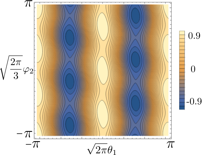
The neutral sector works analogously. We focus on the chiral clock model phenomenology arising for $g_{\bar{3}}>0$, a regime suggested by the contributions of strong repulsive total-density interactions. In the absence of chirality ($g_{1}=0$), a gap arises for large $|g_{2}|\gg g_{\bar{3}}$; in this case the fields $(\sqrt{2\pi}\theta_{1},\sqrt{6\pi}\varphi_{2})$ are locked to the configuration $\pi[n_{x},n_{x}+2n_{y}+\Theta(g_{2})]$. For large $g_{\bar{3}}\gg|g_{2}|$, the system is gapless if $g_{1}=0$ and has central charge $c=1$. These features for $|g_{2}|\gg g_{\bar{3}}$ and $g_{\bar{3}}\gg|g_{2}|$ are similar to those of the ordered and incommensurate phases of the nonchiral regimes of the clock model, respectively. Furthermore, the chiral coupling $g_{1}\neq 0$ can open a gap for $g_{\bar{3}}\gg|g_{2}|$ (with locking configuration $\pi[n_{x}+\frac{1}{2},n_{x}+2n_{y}-\frac{1}{2}\text{sgn}(g_{1})]$), while for $|g_{2}|\gg g_{\bar{3}}$ it can close the gap (provided $|g_{1}|\approx|g_{2}|$), similarly to the effects of chiral deformations on the incommensurate and ordered phases of the clock model. The neutral part of $\mathcal{V}$ for $g_{\bar{3}}\gg|g_{2}|$ and $g_{1}\neq 0$ is illustrated in Fig. 3.

The correspondence between the fermions $\psi_{\eta\alpha}$ and the fields $\theta_{\mu}$, $\varphi_{\mu}$ implies that the latter are periodic variables. In particular, $(\theta_{c},\theta_{1},\varphi_{2})\sim(\theta_{c},\theta_{1},\varphi_{2})+\sqrt{\pi}\bm{n}\cdot\bm{\Gamma}$ (together with a suitable shift of the conjugate pairs) where $\bm{n}$ is a vector of integers and $\bm{\Gamma}=\left(\begin{smallmatrix}\sqrt{3}&0&0\\ 0&\sqrt{2}&0\\ 1/\sqrt{3}&-3/\sqrt{2}&1/\sqrt{6}\end{smallmatrix}\right)$. Under this compactification, the six minima in Fig. 3, at a given $\theta_{c}$, are inequivalent. Six inequivalent minima can also be arranged using a single $\theta_{1}$ (and $\theta_{c}$) but doubling the $\varphi_{2}$ interval. The operator $\exp(2\pi i\tilde{N}_{2}/6)$, which commutes with $H_{\text{b}}$, toggles between the six minima in the latter arrangement; since the values of $\tilde{N}_{c,1}$ specify $\exp(2\pi i\tilde{N}_{2}/6)$, for a given $\tilde{N}_{c,1}$ there is a single ground state corresponding to a superposition between the six minima. The presence of $\mathbb{Z}_{3}$ symmetry, however, guarantees the conservation only of $\tilde{N}_{1}\text{ mod }3$; e.g., boundary terms (or corresponding neutral-sector boundary conditions) generically couple states with $\tilde{N}_{1}$ and $\tilde{N}_{1}+3$. For fixed particle number $\tilde{N}_{c}$, we are thus left with three towers of excitations, each labeled by its $\mathbb{Z}_{3}$ eigenvalue.

Zero modes.- A $\mathbb{Z}_{3}$ label in itself does not imply degeneracies in the spectrum. However, a threefold degeneracy arises if a zero-mode operator $\chi$ exists that commutes with the Hamiltonian while toggling the $\mathbb{Z}_{3}$ label. To obtain such zero modes, we consider the ground-state projections $\chi_{0,\ell}$ of neutral operators at the edge ($x=0,\ell$), taking operators that change $\tilde{N}_{1}\text{ mod }3$. Neutrality ensures maintaining a fixed particle number, while being at the edge means that $\chi_{0,\ell}$ create in $(\theta_{1},\varphi_{2})$ only boundary kinks, a feature compatible Lindner et al. 2012; Cheng 2012; Clarke et al. 2013; Mong et al. 2014 with commutation with at least the groundstate (or, more generally, sub-gap) sector of the Hamiltonian. As in parafermion systems, there are several choices for $\chi_{0,\ell}$ Mong et al. 2014. We choose $\chi_{0,\ell}$ as the ground-state projection of an operator $\mathcal{O}_{\tau}(x=0,\ell)$ in the expansion of $f_{1}^{\dagger}f_{2}$, with $\mathcal{O}_{\tau}^{\dagger}\propto e^{i\frac{1}{3}\sqrt{12\pi}\theta_{c}}e^{i\sqrt{2\pi}\varphi_{1}}e^{i\frac{1}{3}\sqrt{6\pi}\theta_{2}}$. Hence, $\chi_{0,\ell}$ are local operators with $\chi_{0}\chi_{\ell}=\chi_{\ell}\chi_{0}$. They also satisfy $\chi_{0,\ell}\mathcal{S}=\omega\mathcal{S}\chi_{0,\ell}$, the requisite toggling of the $\mathbb{Z}_{3}$ label. By introducing the nonlocal combination $\chi_{\ell}^{\prime}=\mathcal{S}\chi_{\ell}$, we can also use a pair of mutual $\mathbb{Z}_{3}$-parafermions: $\chi_{0}\chi_{\ell}^{\prime}=\omega\chi_{\ell}^{\prime}\chi_{0}$. The phenomenology recovered here matches that of the chiral clock model Fendley 2012; Fendley 2014; Fendley 2016; Alicea and Fendley 2016, including the nonlocal nature of its parafermions. However bosonization indicates the zero-mode character of $\chi_{0,\ell}^{(\prime)}$ only for sub-gap energies, which is sufficient only for their status as “weak” zero modes Alicea and Fendley 2016. To study whether strong zero modes emerge, and for a concrete illustration of our bosonization phenomenology, we next turn to our microscopic model Eq. (Strong zero modes from geometric chirality in quasi-one-dimensional Mott insulators).

Strong-interaction perturbation theory.- We work deep in the Mott insulator regime, $U\gg|J|$. We start with $J=J_{\perp}=V_{a}=0$ in Eq. (Strong zero modes from geometric chirality in quasi-one-dimensional Mott insulators). This limit has a highly degenerate multiplet of lowest-energy states, each with one fermion per site. Turning on a small $V_{a}$ and $J_{\perp}$ splits the low-energy states, without coupling to high-energy states with more than one fermion per site. In contrast, intraleg tunneling $H_{J}=-\frac{J}{2}\sum_{a,i}c_{i,a}^{\dagger}c_{i+1,a}+\text{H.c.}$ connects low- and high-energy states. To obtain the Hamiltonian governing the physics of low-energy states, we perform perturbation theory in $J/U$. The first nonzero correction is in second order in $J/U$, corresponding to a $\mathbb{Z}_{3}$ analogue of superexchange. We find the effective Hamiltonian

valid for $U\gg|V_{a}|,|J|,|J_{\perp}|$.

Using the single occupation per site constraint, $\sum_{a}n_{j,a}=1$, we can rewrite $H_{\rm eff}$ in a form where the relation to the chiral clock model becomes manifest supplementary. We map fermion bilinears to matrices $c^{\dagger}_{j,a}c_{j,b}\rightarrow M_{j}^{ab}$, with components $(M_{j}^{ab})_{kl}=\delta_{ak}\delta_{bl}$ (omitting factors of identity away from site $j$). We find

where we have used Eq. (2) and $N=\ell/a_{0}$. Here $\tau_{j}$ and $\sigma_{j}$ are the clock variables

while $P_{j,j+1}|a\rangle_{j}|b\rangle_{j+1}=|b\rangle_{j}|a\rangle_{j+1}$ is the swap operator between neighboring sites. For $J=0$, Eq. (5) recovers the three-state quantum clock model. It is chiral for $\Phi\neq 0\text{ mod }\pi/3$ Fendley 2012; Alicea and Fendley 2016. Eqs. (2) and (5) thus explicitly establish the link between geometric and clock-model chirality. For $J\neq 0$, the clock model is perturbed by the Uimin-Lai-Sutherland Hamiltonian Uimin 1970; Lai 1974; Sutherland 1975, seen to arise here from superexchange.

For $J=0$, weak $J_{\perp}$, and $\Phi$ sufficiently away from $0\text{ mod }\pi/3$, the system supports strong zero modes with the same properties as that of $\chi_{0,\ell}^{(\prime)}$ above Fendley 2012. Our next goal is to assess whether these strong zero modes survive the superexchange perturbation. We expect this for $|V^{\prime}\sin(3\Phi)|\gg|J_{\perp}|,J^{2}/U$: here the combination of the spectral separation between various $J=J_{\perp}=0$ domain-wall sectors and the scale separation between the chirality-induced intra-sector splittings versus small $|J_{\perp}|,J^{2}/U$ might offer protection also against small nonzero $J$ thanks to the restricted manner in which the swap operation acts on domain-wall states supplementary. To assess the presence of strong zero modes, we first perform exact diagonalization to study the energy spectrum in this regime (Fig. 4a). The existence of a zero mode that arranges the spectrum in $\mathbb{Z}_{3}$ triplets is manifest, both for the three lowest-lying states whose energy splitting decays consistently with an exponential in $N$, as well as for higher energies where the much smaller triplet splitting is almost invisible on the scale of the figure. Our findings are further corroborated by the $5<N<100$ excited-state spectrum in the single-domain-wall sector, where the $\mathbb{Z}_{3}$-triplet splittings decay exponentially with $N$ to a value numerically indistinguishable from zero supplementary.

We next study dynamical consequences of these zero modes. Their edge-mode nature and exchange properties with $\mathcal{S}=\prod_{j=1}^{N}\sigma_{j}$ suggest that they contribute significantly to $\tau_{j}$ at the boundary (in fact, $\tau_{1,N}$ are commuting zero modes for $J=J_{\perp}=0$ Fendley 2012; Alicea and Fendley 2016, akin to $\chi_{0,\ell}$). We compute the infinite-temperature correlator Kemp et al. 2017; Else et al. 2017

where $E_{j}$ is the energy of the eigenstate $|j\rangle$. Time-independent contributions to the correlator come only from $|k\rangle$, $|j\rangle$ in degenerate triplets, provided $\langle k|\tau_{1}|j\rangle\neq 0$. (Diagonal matrix elements vanish due to $\tau_{1}\mathcal{S}=\omega\mathcal{S}\tau_{1}$.) For the signal to be appreciable, $\langle k|\tau_{1}|j\rangle\neq 0$ should hold for many degenerate triplets. In Fig. 4b we show the numerically evaluated correlator for two values of the parameters. (The behavior is similar for other values in the $|V^{\prime}\sin(3\Phi)|\gg|J_{\perp}|,J^{2}/U$ regime, even for weakly disordered systems supplementary.) The results are consistent with the correlator remaining close to its initial value for times exponentially long in system size. Such behavior indicates exponentially decaying triplet splittings across the whole spectrum, and thus illustrates how strong zero modes lead to long-time coherence far from the ground state.

Conclusions.- We have shown how geometric chirality in a $\mathbb{Z}_{3}$- and $\mathcal{T}$-invariant Mott insulator can lead to chiral quantum clock model physics, including strong zero modes. We illuminated this from two complementary perspectives: bosonization based on general symmetry considerations, and the analysis of the model Eq. (Strong zero modes from geometric chirality in quasi-one-dimensional Mott insulators) for strong interactions $U\gg|J|$. In our bosonization, after implementing the Mott-insulating regime by gapping out the charge degrees of freedom, we uncovered fingerprints of the ordered and incommensurate phases of the chiral quantum clock model, and established the presence of zero modes in the ordered phase. This suggests that chiral interactions provide a favorable setting for chiral-quantum-clock-model physics to arise in Mott insulators. Our model Eq. (Strong zero modes from geometric chirality in quasi-one-dimensional Mott insulators) gives concrete evidence for this: for $U\gg|J|$, we explicitly recover the chiral quantum clock model, perturbed by the Uimin-Lai-Sutherland Hamiltonian via superexchange. Our simulations suggest that the strong zero modes survive the superexchange perturbation, leading to the correlators of clock operators at the edge to persist near their initial value for times exponentially long in system size, even at infinite temperature. Interesting directions for future research include the study of the phase diagram and dynamics of our model with approaches that probe the thermodynamic limit. This will, in particular, illuminate where the zero modes we found fall in the refined “strong” versus “almost strong” classification of Refs. Kemp et al. 2017; Else et al. 2017.

We acknowledge discussions with D. Gutman, K. Snizhko, F. Buccheri, and J. Park, and we thank P. Fendley for feedback on the manuscript. This work was supported by the ERC Starting Grant No. 678795 TopInSy.

References

- Fendley (2012) P. Fendley, J. Stat. Mech. 2012, P11020 (2012).
- Fendley (2014) P. Fendley, J. Phys. A: Math. Theor. 47, 075001 (2014).
- Fendley (2016) P. Fendley, J. Phys. A: Math. Theor. 49, 30LT01 (2016).
- Alicea and Fendley (2016) J. Alicea and P. Fendley, Annu. Rev. Condens. Matter Phys. 7, 119 (2016).
- Kemp et al. (2017) J. Kemp, N. Y. Yao, C. R. Laumann, and P. Fendley, J. Stat. Mech. 2017, 063105 (2017).
- Else et al. (2017) D. V. Else, P. Fendley, J. Kemp, and C. Nayak, Phys. Rev. X 7, 041062 (2017).
- (7) J. Kemp, N. Y. Yao, and C. R. Laumann, arXiv:1912.05546 .
- (8) D. J. Yates, A. G. Abanov, and A. Mitra, arXiv:2002.00098 .
- Wootton and Pachos (2011) J. R. Wootton and J. K. Pachos, Phys. Rev. Lett. 107, 030503 (2011).
- Stark et al. (2011) C. Stark, L. Pollet, A. Imamoğlu, and R. Renner, Phys. Rev. Lett. 107, 030504 (2011).
- Bauer and Nayak (2013) B. Bauer and C. Nayak, J. Stat. Mech. , P09005 (2013).
- Huse et al. (2013) D. A. Huse, R. Nandkishore, V. Oganesyan, A. Pal, and S. L. Sondhi, Phys. Rev. B 88, 014206 (2013).
- Parameswaran et al. (2017) S. A. Parameswaran, A. C. Potter, and R. Vasseur, Ann. d. Phys. 529, 1600302 (2017).
- Alet and Laflorencie (2018) F. Alet and N. Laflorencie, C. R. Phys. 19, 498 (2018).
- Parameswaran and Vasseur (2018) S. A. Parameswaran and R. Vasseur, Rep. Prog. Phys. 81, 082501 (2018).
- Abanin et al. (2019) D. A. Abanin, E. Altman, I. Bloch, and M. Serbyn, Rev. Mod. Phys. 91, 021001 (2019).
- (17) T. B. Wahl and B. Béri, arXiv:2001.03167 .
- Lindner et al. (2012) N. H. Lindner, E. Berg, G. Refael, and A. Stern, Phys. Rev. X 2, 041002 (2012).
- Cheng (2012) M. Cheng, Phys. Rev. B 86, 195126 (2012).
- Clarke et al. (2013) D. J. Clarke, J. Alicea, and K. Shtengel, Nat. Comm. 4, 1348 (2013).
- Mong et al. (2014) R. S. K. Mong, D. J. Clarke, J. Alicea, N. H. Lindner, P. Fendley, C. Nayak, Y. Oreg, A. Stern, E. Berg, K. Shtengel, and M. P. A. Fisher, Phys. Rev. X 4, 011036 (2014).
- Tsvelik (2014) A. M. Tsvelik, Phys. Rev. Lett. 113, 066401 (2014).
- Klinovaja and Loss (2014) J. Klinovaja and D. Loss, Phys. Rev. Lett. 112, 246403 (2014).
- Zhang and Kane (2014) F. Zhang and C. L. Kane, Phys. Rev. Lett. 113, 036401 (2014).
- Orth et al. (2015) C. P. Orth, R. P. Tiwari, T. Meng, and T. L. Schmidt, Phys. Rev. B 91, 081406 (2015).
- Alexandradinata et al. (2016) A. Alexandradinata, N. Regnault, C. Fang, M. J. Gilbert, and B. A. Bernevig, Phys. Rev. B 94, 125103 (2016).
- Alavirad et al. (2017) Y. Alavirad, D. Clarke, A. Nag, and J. D. Sau, Phys. Rev. Lett. 119, 217701 (2017).
- Calzona et al. (2018) A. Calzona, T. Meng, M. Sassetti, and T. L. Schmidt, Phys. Rev. B 98, 201110 (2018).
- Mazza et al. (2018) L. Mazza, F. Iemini, M. Dalmonte, and C. Mora, Phys. Rev. B 98, 201109 (2018).
- Hutter and Loss (2016) A. Hutter and D. Loss, Phys. Rev. B 93, 125105 (2016).
- Alicea and Stern (2015) J. Alicea and A. Stern, Physica Scripta 2015, 014006 (2015).
- Chew et al. (2018) A. Chew, D. F. Mross, and J. Alicea, Phys. Rev. B 98, 085143 (2018).
- Santos et al. (2019) R. A. Santos, D. B. Gutman, and S. T. Carr, Phys. Rev. B 99, 075129 (2019).
- Jermyn et al. (2014) A. S. Jermyn, R. S. K. Mong, J. Alicea, and P. Fendley, Phys. Rev. B 90, 165106 (2014).
- Zhuang et al. (2015) Y. Zhuang, H. J. Changlani, N. M. Tubman, and T. L. Hughes, Phys. Rev. B 92, 035154 (2015).
- Moran et al. (2017) N. Moran, D. Pellegrino, J. K. Slingerland, and G. Kells, Phys. Rev. B 95, 235127 (2017).
- Fendley et al. (2004) P. Fendley, K. Sengupta, and S. Sachdev, Phys. Rev. B 69, 075106 (2004).
- Lecheminant and Nonne (2012) P. Lecheminant and H. Nonne, Phys. Rev. B 85, 195121 (2012).
- Tsvelik and Kuklov (2012) A. M. Tsvelik and A. B. Kuklov, New J. Phys. 14, 115033 (2012).
- Samajdar et al. (2018) R. Samajdar, S. Choi, H. Pichler, M. D. Lukin, and S. Sachdev, Phys. Rev. A 98, 023614 (2018).
- Keesling et al. (2019) A. Keesling, A. Omran, H. Levine, H. Bernien, H. Pichler, S. Choi, R. Samajdar, S. Schwartz, P. Silvi, S. Sachdev, et al., Nature 568, 207 (2019).
- Buda et al. (1992) A. B. Buda, T. A. der Heyde, and K. Mislow, Angew. Chem. 31, 989 (1992).
- Saito et al. (1998) R. Saito, G. Dresselhaus, and M. S. Dresselhaus, Physical properties of carbon nanotubes (World Scientific, 1998).
- Fasman (2013) G. D. Fasman, Circular dichroism and the conformational analysis of biomolecules (Springer, 2013).
- (45) The model is also invariant under reflection along the legs combined with exchanging two of the legs; this symmetry can be used instead of time-reversal in our considerations.
- Giamarchi (2003) T. Giamarchi, Quantum Physics in One Dimension (Clarendon Press, 2003).
- Gogolin et al. (2004) A. Gogolin, A. Nersesyan, and A. Tsvelik, Bosonization and Strongly Correlated Systems (Cambridge University Press, 2004).
- (48) The model’s single-particle Hamiltonian has a reflection symmetry which leads to ; however, this is not a generic feature. All the processes we consider survive in the more general - and time-reversal-invariant case with split and .
- Teo and Kane (2014) J. C. Y. Teo and C. L. Kane, Phys. Rev. B 89, 085101 (2014).
- Fabrizio and Gogolin (1995) M. Fabrizio and A. O. Gogolin, Phys. Rev. B 51, 17827 (1995).
- Uimin (1970) G. V. Uimin, JETP Lett. 12, 225 (1970).
- Lai (1974) C. K. Lai, J. Math. Phys. 15, 1675 (1974).
- Sutherland (1975) B. Sutherland, Phys. Rev. B 12, 3795 (1975).
- (54) See Supplemental Material for details on the correspondence between Eq. (4) and Eq. (5), our domain-wall considerations, and for additional numerical results.
Supplemental Material
In this Supplemental Material we explain the correspondence between Eq. (4) and (5) of the main text, and provide further corroborating evidence complementing that in Fig. 4 of the main text.
I From the fermion Hamiltonian to the perturbed quantum clock model
In the main text we note that the constraint of single occupation per site, , allows us to rewrite the fermion Hamiltonian [Eq. (4) of the main text] in the form of a perturbed chiral quantum clock model [Eq. (5) of the main text] using a map between fermion bilinears and matrices . In this section, we provide the details behind these observations.
The matrix is understood as