Modeling and detecting resonant tides of exotic compact objects
Abstract
The event horizon of a black hole in general relativity absorbs all infalling radiation. Any observation of the contrary would immediately challenge the expectation that astrophysical black holes are described by the vacuum Kerr geometry. If a putative black hole does reflect part of the ingoing radiation, its quasinormal mode structure is drastically altered. Low frequency modes can be introduced that are resonantly excited during the inspiral of a binary system. We study the resulting phase shift of the gravitational wave signal. Building on neutron star results, we obtain a model-independent expression for the phase shift that depends only on quasinormal modes and Love numbers of the compact object. We find that the phase shift might be detectable with Einstein Telescope for asymmetric binaries in high signal-to-noise events (), but by far cannot explore the Planck scale.
I Introduction and summary
A fundamental question of present-day research concerns the nature of astrophysical black holes: are they truly described by the Kerr family of General Relativity? The ever-increasing precision of gravitational wave experiments is a sensitive probe that offers insight into this question. A rich phenomenology has sprouted in recent years on horizonless compact objects, which have some structure close to the would-be event horizon, and can serve as testable alternatives to the Kerr paradigm. Many of the models for such exotic compact objects (ECO) are directly inspired or even predicted by fundamental physics models that describe new physics near black holes, ranging from dark matter to quantum gravity Morris1988, Mazur2001, Schunck:2003kk, Mathur2005, Barcelo2007, Barcelo:2010vc, Barcelo:2014cla, Holdom:2016nek, Raposo:2018xkf, Liebling:2012fv, Cardoso:2019rvt, PhysRevLett.66.1659, Gleiser:1993pt, Seidel:1993zk. Exploring their gravitational wave signatures transforms compact merger events into fundamental physics laboratories.
A main theme in this exploration is to find model-independent gravitational wave (GW) observables that can distinguish an exotic compact object from a black hole. Two key sets of observable that have been studied recently are GW echoes following the merger and tidal effects during inspiral. GW echoes Cardoso2016(2), Cardoso2016, Cardoso2017, Conklin:2017lwb, Mark:2017dnq, Price:2017cjr, Wang:2018mlp, Wang:2019szm, Bueno:2017hyj, Ashton:2016xff, Maggio:2019zyv arise when the ECO reflects part of the incoming gravitational radiation: the interaction between the ECO and its light ring behaves as a resonant cavity inducing a particular set of trapped quasi-normal modes (QNM) of significantly lower frequency than the standard black hole QNMs. Potentially observable with LIGO/Virgo, the data analysis hunt is on, with no conclusive evidence up to date Abedi:2016hgu, Abedi:2017isz, Ashton:2016xff, Uchikata:2019frs, Lo:2018sep, Nielsen:2018lkf, Testa:2018bzd, Tsang:2018uie, Westerweck:2017hus. Adiabatic tidal interactions on the other hand can lead to deformability and heating effects which typically appear in the GW signal as highly suppressed corrections during most of the inspiral. Those effects are in principle detectable with 3G detectors Cardoso:2017cfl, Maselli:2017cmm, Johnson-McDaniel:2018uvs, Maselli:2018fay, Datta:2019epe, Datta:2020gem, Pani2010, Cardoso:2019nis, Pons2002, Gualtieri2001, Flanagan2007, Cardoso2017(2), Binnington2009, flanagan2008, Damour2009, Cardoso:2019nis, Datta:2019euh, Ruoff2000, Kokkotas1995.
The same physical mechanism underlying GW echoes offers the possibility for another effect in the inspiral phase: low frequency QNMs can be excited by the driving of the companion. At resonance, tidal effects suddenly become more dominant. This gives two potentially observable effects. First, sharp peaks in the emitted gravitational wave power are to be expected when the orbital frequency matches the resonant frequency of an internal oscillation mode of the object. This effectively leads to a high frequency ‘glitch’ in the observed signal which is most likely inaccessible to current or planned detectors Cardoso:2019nis. Second, the significant enhancement of energy in an internal mode causes a phase difference in the GW signal. This kind of resonance phenomenon has already been discussed at length in the context of neutron stars (NS) Kojima1987, Reisenegger1993, Lai1994, Pons2002 and white dwarfs Rathore:2004gs, and numerically for particular ECO models such as gravastars and boson stars Cardoso:2017cfl, Cardoso2017, Pani2010, Macedo2013, Cardoso2016. A recent model-independent data analysis for the phase shift due to inspiral resonances showed no deviation from GR in second-generation GW observations yet NikhefResonances. However, a detailed treatment for the form and expected size of the phase shift for generic compact objects is currently not available.
In this paper, we investigate specifically the perspectives for detection of the phase shift induced by a resonant excitation of the heaviest object in a comparable mass binary merger. The companion could be a black hole, a neutron star or even another ECO although tidal effects in the companion will not be taken into account. By extrapolating known results for neutron stars, we write down the phase shift in terms of QNMs and Love numbers of the ECO. We determine the prospects for detection of those modes using ground-based GW detectors using a Fisher analysis. Although our setup is more generally valid, we do this analysis for the simplest model of a reflecting surface at coordinate radius where is the ECO mass, will be the companion mass, and is a dimensionless parameter controlling the compactness of the ECO or alternatively a “closeness” parameter that indicates how close the reflective surface is to the would-be horizon Cardoso:2019rvt. In particular, is chosen such that the surface lies well within the photonsphere but is, in proper distance, more than a Planck length away from the putative horizon. For a hundred solar mass object, this implies lies roughly between and . We find that with current detector capacity observation of the phase shift of our model is ruled out. With third generation GW observatories, things look better but might still be out of reach. We focus on Einstein telescope and find that only at high signal-to-noise ratios of the phase shift becomes detectable for mass ratios of roughly and a wide range of , but nevertheless corresponding to a proper distance away from the horizon of many orders of magnitude above Planck scale. The phase shift at leading order in scales with the inverse of the mass ratio, suggesting better prospects for extreme mass ratio inspirals (EMRI) with LISA. However, our approximations do not extend to that setup and we defer a proper EMRI study to future work. Along the way, we also discuss how the resonance can be written in an effective theory as is done for GW echoes. We explore the post-Newtonian structure of this approach and, thereby, clarify how the dynamic tidal deformability induces a difference in gravitational wave emission between an ECO and a black hole at resonance.
The rest of the paper discusses our main points as follows. In section II, we discuss the inspiral of a featureless point particle into a compact object. After a quick review of the linear response to the tidal field of the companion, we model the ECO as a point particle dressed with multipolar deformation degrees of freedom. Such a description is applicable irrespective of the details of the object and has been developed and applied previously for stellar objects Goldberger2004. Following this previous literature we derive the phase shift as consequence of a resonance in the GW signal by estimating the orbital energy that leaks into a specific mode of oscillation. For neutron stars, this driving is known to be related to the overlap integrals that describe the internal structure of the object Flanagan2007, Chakrabarti2013u1306. By assuming only the fundamental mode contributes, we express the overlap integrals in terms of the Love numbers to arrive at a largely model-independent estimate of the phase shift, see equation (II.19b) below.
In section III, we discuss the essential difference with stellar objects in the form of the tidal response function. This requires input depending on the nature of the object itself. We give a near-zone analysis of the object, closely following the discussion in Mark:2017dnq developed for GW echoes, and characterize an ECO by its boundary conditions that replace the purely absorbing black hole horizon. We show how, in a low frequency limit, the transfer function of Mark:2017dnq is proportional to the linear response function of the effective theory of quadrupole deformations, elucidating the relation to the high-frequency glitch described in Cardoso:2019nis and tidal effects in the post-Newtonian expansion. For calculational reasons, we focus on the EMRI limit in this section.
In section IV, we first discuss the basic conditions that have to be satisfied for a resonance to be seen in a gravitational wave signal, including relation to mass and details of central object and ECO. We restrict to a simple model and qualitatively observe that such a detection is possible in principle. However, we then perform a Fisher analysis and find that the resulting phase shift is unlikely to be seen by the Einstein Telescope.
II Harmonic oscillator model of a compact object
We first give a quick recap of the phase shift derived using the Newtonian approximation Lai1994, Reisenegger1993, Flanagan2007 and the harmonic oscillator model used to describe the linear response of stellar objects subject to a tidal field Chakrabarti2013, Chakrabarti2013u1306, steinhoff2016. We end by expressing the phase shift in terms of the GR Love numbers and mode frequencies.
The reader interested in the results can jump to section II.3.
II.1 Phase shift in the Newtonian approximation
We consider two masses and with mass ratio . In the early inspiral, the motion is dominated by the point-particle motion at the leading (post-)Newtonion order. On the additional assumption of quasi-circular orbits, it is described by the relative separation of the masses, , and the orbital phase, :
| (II.1a) | ||||
| (II.1b) | ||||
in which and are the time and phase of coalescence respectively, is the chirp mass and the reduced mass given by
| (II.2) |
Now consider to be an ECO that can be equipped with additional internal degrees of freedom, will still be modeled as a featureless point particle. A resonant excitation of an internal degree of freedom during the inspiral effectively causes a phase shift in the gravitational wave signal; the GW phase away from the resonance regime is given by Flanagan2007
| (II.3) |
where estimates the duration of resonance, is the angular velocity of the binary evaluated at resonance and is the GW phase as predicted for a point-particle. Our order-of-magnitude estimate for the phase shift is
| (II.4) |
in which is the ‘Newtonian’ gravitational wave luminosity and denotes the orbital energy loss in a particular, resonantly excited, -multipole mode. The second factor is the time scale associated to the energy loss during normal GW emission hence estimates the shift in GW phase when passing through a resonance epoch. We will obtain the energy loss from a linearized harmonic oscillation model put forward in Chakrabarti2013u1306 on assuming the no back-reaction approximation (the orbital motion of the companion is a constant supply of energy without the mode oscillations influencing the orbit).
II.2 Oscillating stars
Chakrabarti et al. Chakrabarti2013u1306 have shown how to incorporate multipolar degrees of freedom on the worldline of a point particle to describe a generically deformed object in the Newtonian regime (this will naturally restrict us to tidal effects of electric type). Fundamental quantities are the deformation amplitudes of a specific normal mode of oscillation and the (quasi) normal modes of the central object . Note that the QNMs do not carry an -index because of assumed spherical symmetry of the ECO. In the regime of linear response, these amplitudes are described by a driven, damped harmonic oscillator
| (II.5) |
where a dot denotes a time derivative and with the frequency of oscillation and damping coefficients; they are related to the quasi-normal frequencies of the central object as
| (II.6a) | ||||
| (II.6b) | ||||
The driving term describes how the internal degrees of freedom of the central object couple to the external tidal field of the companion Chakrabarti2013u1306. The precise relation is most easily written in a symmetric trace-free (STF) tensor basis where is a multi-index and the hat denotes STF projection, see section IV and/or appendix A of Chakrabarti2013u1306 for a more detailed description. The driving term is given by
| (II.7) |
In this expression, is the overlap integral encoding equation of state information of the central object, the hatted refers to the STF projection of a multi-index partial derivative11 1 For instance, applying this notation to a partial differential , with taking values in ,, and the Cartesian coordinates of . This is, however, simply equal to when acting on a Newtonian potential in vacuum. and is the Newtonian gravitational potential of the companion evaluated at its position , in particular
| (II.8) |
We will focus only on quasi-circular orbits in the equatorial plane. This simplifies the driving term to the split form
| (II.9a) | |||
| where the amplitude is given by | |||
| (II.9b) | |||
| and where and are given in (II.1) and is a numerical prefactor | |||
| (II.9c) | |||
Note that we take the modulus of the overlap integral when compared to (II.7). Any phase corresponding to can be absorbed in the definition of the orbital phase (II.1b).
When a solution to the oscillator equation (II.5) is obtained, the energy stored in the -mode can be obtained in the standard fashion from the solution of (II.5) as follows
| (II.10) |
The energy in the modes after passing through a resonance can be approximated by Rathore:2004gs, Reisenegger1993
| (II.11) |
where is the Heaviside step function given by
| (II.12) |
and
| (II.13) |
Here, and are respectively the driving amplitude, see (II.9a), and change in angular velocity of the binary evaluated at resonance. Note that gives the total amount of energy transferred from the orbit to the mode while is the present amount of energy in the mode (that is, the total amount minus the amount which is dissipated by internal friction or gravitational wave emission). Using this result (II.13) for the phase shift estimate (II.4) yields
| (II.14) |
This expression depends on the overlap integrals and hence on the internal structure and mass distribution of the central object .
II.3 From stars to compact objects
To make contact to ECOs, we express the overlap integrals in (II.14) in terms of the Love numbers using the effective theory of tidal deformations. To this end, we will restrict to fundamental modes22 2 We choose the convention for the fundamental mode as it is convenient to describe the trapped QNM’s in (IV.2). However, this means a shift is required in the comparison with the traditional choice for stellar oscillations. and omit the subscript henceforth.
For quadrupolar deformations in GR, one can construct an effective action for a dynamical quadrupole degree of freedom on the wordline of a point particle (in our case: the ECO). The linear response to an external tidal field is given through the following coupling with the electric component of the Weyl tensor , in the frequency domain
| (II.15) |
where we have used , to indicate the Fourier transforms of , and is the linear response function, in the frequency domain, that determines the strength of the tidal interaction and depends on the properties of the compact object, such as its equation of state.
In the low-frequency regime, the Taylor expansion of gives the tidal constants:
| (II.16) |
with for the relativistic quadrupolar dimensionless electric tidal Love number , related to absorption and parametrizing tidal response beyond the adiabatic limit Chakrabarti2013. Note that the relativistic tidal Love numbers of non-spinning objects can be split in to two classes based on parity: electric (even-parity) and magnetic (odd-parity). We only consider the electric type as they also exist in the Newtonian theory, in contrast to the magnetic-type Love numbers Pani:2018inf. Furthermore, we use the convention for of Cardoso:2017cfl, where it is shown explicitly how this convention differs, for example, from the conventions of Binnington2009, Hinderer:2007mb. Near resonance, the response function has a pole structure,
| (II.17) |
with the resonant frequencies. As indicated, the residues are related to the overlap integrals. By equation (II.16) and (II.17), we can then immediately relate Love number and overlap integral.
For generic multipoles, we use the Newtonian limit of Chakrabarti2013u1306. In appendix B, we list those results and repeat the above reasoning. The main assumption made is that overlap integrals for fundamental modes dominate above their overtones; hence we truncate to . The overlap integral is given as:
| (II.18) |
with the electric mutipolar Love numbers. The phase shift (II.14) becomes
| (II.19a) | |||
| where the numerical prefactor is given by | |||
| (II.19b) | |||
The numerical factor is given in equation (II.9c).
We have made the assumption that the same relations as for Newtonian stars holds for ECO’s. However, the tidal behaviour of ECOs is counterintuitive compared to normal Newtonian fluid objects, in particular the Love numbers for very compact objects can actually become negative (see eq. (IV.3) below). Therefore we work with the square of the overlap integral and take the modulus in (II.19a) to have the correct physical sign of the phase shift. It would be interesting to perform an independent check of the complex nature of the overlap integrals for ECOs by evaluating the residues in the response function explicitly (II.17).
III Resonances of Exotic Compact Objects
For simplicity, we keep the discussion focused on a non-rotating ECO. Section III.1 reviews relevant elements of previous work, mainly Mark:2017dnq, while introducing our notation. It also stresses the natural relation between echoes and low frequency resonances. Subsequently, in section III.2, we make a connection between that approach and the effective harmonic oscillator model presented in section II. That relation is elegantly summarized, in the low frequency limit, by (III.23). Finally, in III.3, we exhibit the enhanced gravitational wave flux that was also discussed in Cardoso:2019nis as well as indicate how it suggests a resummation of the post-Newtonian expansion with dynamical tides.
III.1 Perturbing an ECO
Gravitational perturbations around a non-rotating black hole background are governed by the Regge-Wheeler (RW) equation regge1957,
| (III.1) |
with
| (III.2) |
and the tortoise coordinate . We will denote the radial coordinate of the horizon as . The frequency domain Regge-Wheeler function can be straightforwardly connected to linearized metric perturbations around a Schwarzschild background for the odd-parity sector in Regge-Wheeler gauge Martel:2005ir
| (III.3) |
with , the area form on the unit two-sphere, the index running over the angular coordinates and the complex conjugate of the parity-odd vector spherical harmonics, which can be constructed from the ordinary spherical harmonics by
| (III.4) |
with , respectively the covariant derivative and the Levi-Civita tensor on the unit two-sphere. For the even-parity sector, the relation is more complicated but can nevertheless be found through the Chandrasekhar transformation chandrasekhar1975. The source term can similarly be connected to the stress-energy tensor but consider, for the moment, the homogeneous equation (III.1) with . Two independent solutions are given asymptotically by
| (III.5a) | |||
| (III.5b) |
Here, the asymptotically outgoing and ingoing amplitudes, , of as well as the horizon outgoing and ingoing amplitudes , of also depend on although this is left implicit for notational simplicity. The solutions introduced in (III.5b) have the right boundary conditions for a black hole respectively at the horizon and asymptotically. However, for a compact object distinct from a black hole, (III.1) is only valid up until a particular and one must impose an alternative boundary condition. We will denote the homogeneous solution satisfying this boundary condition . To go from the black hole to the exotic compact object then essentially amounts to replacing with . Since for generic frequencies and are independent, one can generally express as a linear combination of both. As by assumption is close to , we will follow the notation of Mark:2017dnq and characterize this homogeneous solution with the correct boundary conditions at the ECO as
| (III.6) |
with an arbitrary function of the frequency and the mode numbers . For instance, the specific reflectivity of was discussed in Cardoso:2019nis. Note that, despite the apparent remaining freedom, this is a strong reduction of the possible boundary conditions as in general they could be nonlinear functions of all other modes .
Given an understanding of the compact object, one can exactly determine what the boundary condition expressed through (III.6) should be by imposing appropriate regularity conditions inside the object and matching this to our exterior description as in the examples of neutron stars Gualtieri2001, gravastars Pani2010 or boson stars Macedo2013. Alternatively, one could encode this information by continuing beyond but with an alternative potential which effectively captures certain interesting features as in volkel2017. We will keep the discussion general on the level of this boundary condition following Mark:2017dnq.
Consider (III.1) in the presence of a source . Given such a source term, one can solve (III.1) with variation of parameters using the homogeneous solutions with the appropriate boundary conditions. For a black hole this gives
| (III.7a) | ||||
| with the wronskian | ||||
| (III.7b) | ||||
Instead, for the ECO, using the same procedure in combination with (III.6) one finds
| (III.8) |
with
| (III.9) |
and with the black hole reflection and transmission amplitudes
| (III.10) |
An observer measuring gravitational waves at would see the black hole as
| (III.11) |
with
| (III.12) |
On the other hand, for the exotic compact object we have
| (III.13) |
with
| (III.14) |
Two crucial remarks can be made using the structure of (III.9) Mark:2017dnq. The first is that from the expansion
| (III.15) |
an observer sees an initial perturbation of the ECO decaying as a black hole ringdown followed by a series of echoes spaced by a time interval . Secondly, there are a set of QNMs associated to this characteristic timescales arising from the poles in , particularly from
| (III.16) |
Therefore, one easily relates a specific set of resonant modes in ECO and the phenomenology of echoes. Echoes only truly emerge if is sufficiently close to the horizon or more precisely . This implies that the characteristic frequency is relatively low and this is for our purpose the crucial difference with black hole QNMs. Indeed, BH QNMs are in principle equally susceptible to resonant excitation but this is of less interest in a generic inspiral because the frequencies are too high to be resonantly excited in that stage of the binary evolution (see however the observation of Loutrel2017, Nasipak2019 for highly eccentric inspirals). For the ECO discussed here, on the other hand, the QNM frequencies can be significantly lower such that the resonant frequencies can occur during the inspiral.
III.2 Transfer to tidal response
The proper way to include the companion mass to the previous description, would be to consider it as a near-zone description of and to impose boundary conditions found by a matched asymptotic expansion with an outer-zone33 3 Sometimes the outer-zone is called the near-zone (also orbital-zone) while our near-zone is called the inner-zone (also body-zone). containing . This outer-zone in turn could for instance be described by a post-Newtonian expansion mundim2014. Such a procedure carried out in full, however, becomes cumbersome very quickly and it is more convenient to instead use the near-zone to match to an ‘intermediary’ effective action steinhoff2016. The near-zone features of the ECO in this approach are encoded in the effective (linearized) dynamical tidal response as in (II.15). This tidal response was related explicitly to the asymptotic form of in a expansion by Chakrabarti2013. These authors used the black hole perturbation equations with an effective source to describe the near-zone perturbation equations of neutron stars, but the approach is applicable to more general compact objects. The effective source is determined based on the intermediary effective action by matching the two descriptions in the asymptotic region of the near-zone. This gives the desired relation between and . Concretely, consider the particular basis , of solutions to the homogeneous RW equation (III.1) with asymptotic behavior
| (III.17a) | ||||||
| (III.17b) | ||||||
for some constants , , described explicitly in (A.9). Here, indicates the renormalized angular momentum, which reduces to in the low frequency limit sasaki2003. Naively, one could therefore try to regard , respectively as the tidal field and the multipolar response but it is not straightforward to connect that point of view to the actual radiation zone asymptotic behavior (III.17). Nevertheless, it was shown in Chakrabarti2013 that, defining through
| (III.18) |
can be written in a expansion as
| (III.19) |
This is the leading order of equation (15) in Chakrabarti2013. Comparing (III.18) with our previous expressions (III.5b), (III.6) and (III.9) we find that is related to by
| (III.20) | ||||
It is important that we are assuming a hierarchy of scales in which, even though , the orbital frequency is potentially of similar order as the resonant mode . In particular, it would not be appropriate to expand , as in the adiabatic limit, where it could be essentially replaced by the (quadrupolar) tidal Love number (B.4) as this would be the lowest order in the expansion with respect to the internal fundamental frequency scale as opposed to . For a black hole
| (III.21) |
such that we can write
| (III.22) |
and finally, for , using (III.19) and low frequency expansions for black hole quantities such as , ,44 4 Note that can be replaced by in a low frequency expansion according to (III.19) and, in the same expansion, could be replaced by the associated adiabatic tidal deformability since there for the black hole . Now the tidal Love number of the black hole vanishes leaving a proportionality with . derived for instance in poisson1995, and reviewed for convenience in Appendix A
| (III.23) |
with a numerical factor. We make the derivation of (III.23) more explicit in Appendix A and explain there why we cannot determine the constant a priori. Essentially, it is due to a regularization dependence in (III.19). We instead fix the coefficient to be by matching the energy flux to the post-Newtonian expansion. In conclusion, at least in the limit , the near-zone characterization of the object through is straightforwardly related to the effective field theory description using .
III.3 Enhanced GW flux at resonance
We will now describe how there is also an increase in gravitational wave flux at resonance. This is in particular what was studied in Cardoso:2019nis and found there to give rise to an “unobservable high-frequency glitch". We stress that this is not the same as looking for a phase shift like (II.19b), which does not try to directly measure the variation in gravitational waves. Rather it considers the impact on the orbit and the indirect change in GW phasing associated to this. The same authors also consider the impact of a phase shift in the gravitational wave signal, but only due to the additional energy lost through this enhanced gravitational wave flux during resonance. However, this is not the same as the total energy lost from the orbit at resonance. Even in the simple example of Cardoso:2019nis where no energy is absorbed by the ECO itself, such that eventually all energy in the excitation must be dissipated through gravitational waves. The reason is that this dissipation does not happen instantly at resonance. In fact, the more sharply peaked the resonant frequency, the longer it will take for all this absorbed energy to be radiated. It is therefore more appropriate to consider how much energy goes into the excited mode at resonance, as was done in section II, as opposed to how much of this is immediately radiated at resonance. Nevertheless, the present formalism allows for a perspicuous description of the peak in gravitational wave flux such that we shall take a moment to describe it.
In an extreme mass ratio limit , the source in (III.1) can be constructed from the stress-energy tensor of an orbiting point-particle . If this companion is on a circular orbit with angular frequency , the total gravitational wave luminosity is given by 55 5 This is normally expressed in terms of the analogues of (III.12) and (III.14) starting from the Bardeen-Press-Teukolsky equation bardeen1973, teukolsky1973 which is more convenient in this setup. Nevertheless, treating carefully, one should also be able to find them from (III.12) and (III.14) using the Chandrasekhar transformation chandrasekhar1975 and we do so to avoid introducing unnecessary new notation.
| (III.24) |
Consider the normalized difference of with respect to the expression for a black hole around a particular QNM frequency for a certain mode
| (III.25a) | ||||
| with | ||||
| (III.25b) | ||||
The form of (III.25a) consists of a typical Breit-Wigner peak with an additional interference term. A representative example of this form is shown in figure 1. The result is not surprising and it has been observed in particular cases Pons2002, Pani2010, Macedo2013. The given example highlights that often in these resonances there seems to be a large contribution from the asymmetric interference term in (III.25a). It should be noted that although we have discussed a resonance in the radiated energy, there is also an interesting conservative resonant response in the backreaction on the orbit isoyama2016. Moreover, once the full self-force, including the conservative piece, is known for the black hole, it is evident that one can simply add to this the force associated to the (homogeneous) last term in (III.8), which requires no additional regularization drivas2011dependence. We shall not pursue this point further here.
To intuitively understand this enhanced gravitational wave flux better, let us connect this general extreme-mass ratio formula to its post-Newtonian limit. From the standard low frequency expansions for the black hole quantities, as can be found for instance in poisson1995, in addition to (III.19), one finds that the energy flux (III.24) can be expressed in this limit as
| (III.26) |
Expanding this result further, assuming one is not too close to resonance as to avoid subleading terms including to become significant, one finds
| (III.27) | ||||
where we have made explicit only the leading order contribution, despite the existence of many additional terms leading with respect this. These, denoted by where , would however, simply be the black hole result which are known to very high order, see sasaki2003, for a review. (III.27) can be readily compared to the post-Newtonian expression of GW luminosity for a binary including effects of tidal deformability by using (II.16) in the adiabatic limit
| (III.28) | ||||
For instance, with and flanagan2008
| (III.29) | ||||
Aside from the fact that (III.27) is valid only as , the difference is that (III.27) still captures some of the dynamic aspects of the tidal deformability. It suggests a way of resumming dynamic tidal interactions in a post-Newtonian expansion and resonates well with the introduction of an effective tidal Love number in steinhoff2016. In that paper, was replaced by an effective-Love number function in order to efficiently capture dynamic tidal effects in an effective-one-body approach
| (III.30) |
similar to the response function in (II.15). It would be interesting to investigate how this works out precisely but we shall not pursue this further here.
We can again observe from (III.27) that the enhanced gravitational wave flux at resonance, as expected, is simply because the deformed object has a varying quadrupole moment itself which also contributes to the emitted gravitational waves. This result was derived for a fixed circular orbit. It does not allow us to conclude that, with an evolving orbit, this deformation would simply disappear as the resonance is past. Therefore, it would be incorrect to conclude that all the energy lost to the orbit was simply the additional flux during resonance. Instead, off-resonance, the excited mode will continue to ring down. In itself, this will be too weak to observe directly but in the total energy that was lost to the orbit when the associated energy was transferred to the mode, a measurable phase shift might have been induced into the waveform. This is what we will investigate now.
IV Detectability
To at least get an order of magnitude estimate on the detectability, we will perform a Fisher analysis pinned down to a particular ECO model. The ECO model is the simplest reflecting shell model Cardoso:2019rvt which serves our illustrative purposes although a similar analysis on different models might also be performed.
IV.1 The model
The reflecting shell model is decisively simple, but it nevertheless captures the physics of horizon absence. Phenomenologically, this absence inevitably introduces a certain amount of reflection of incoming waves within the light ring. The simplest model that captures this, is a purely reflecting surface put at a Schwarzschild coordinate where is the mass of the object and is a small dimensionless parameter that quantifies the “closeness” to a black hole spacetime as introduced in section I. The proper distance from the Schwarzschild radius to the reflective surface at in the small limit is given by
| (IV.1) |
The parameter ranges from where is about one Planck length to where the object has a clean photonsphere Cardoso:2017njb. However, in practice our upper limit will be . This will be explained below.
On the level of the wave equation, the surface can be treated effectively by using reflective boundary conditions at and the QNMs in the limit, valid in our range, have been analyzed by Cardoso et al. Cardoso:2019nis
| (IV.2) | ||||
Furthermore, it is also shown that the Love numbers of those objects in the limit take the following approximate form Cardoso2017(2)
| (IV.3) |
where depend on the multipolar index . Note that , the Love numbers are negative. For instance, for quadrupolar deformations for our shell model, it has been found that and Cardoso2017(2). Using this approximation, the phase shift (II.19a) is fully determined by the location of the surface , the mass ratio and the multipolar indices . In particular, from (IV.2), (IV.3) and (II.19a), the mass dependence scales to leading order in as
| (IV.4) |
where the proportionality constant, which only depends on , is about for quadrupolar waves and increases slightly with . From (IV.4), it immediately follows that for small mass ratios, the phase shift is inversely proportional to the mass ratio and the -dependence is such that higher order -modes are at least suppressed by factors of . In particular for our upper limit , it can be computed that higher order -modes are generically suppressed by at least two orders of magnitude
| (IV.5) |
This makes that the largest phase shift comes from quadrupolar excitations, by (IV.4) it can be seen that the phase shift itself has a very weak -dependence. In particular, when runs from Planck scale () to roughly , the phase shift only changes by two orders of magnitude.
IV.2 Criteria for detectability
In order to detect the phase shift, the following criteria should be fulfilled:
- (a)
Resonant excitation should take place at a frequency lower than that at the moment of merger,
- (b)
The resonant frequency should lie within the detector band,
- (c)
The measurement error on should be smaller than itself.
The first condition is purely the statement of the resonant effect happens at all, the others are detector dependent statements. The first condition puts a restriction on in terms of the mass ratio. In particular if one estimates that the plunge initiates at an orbital separation of roughly , then the requirement that the orbital resonant frequency, associated to (IV.2), is smaller than the approximate merging frequency, , translates to
| (IV.6) |
This also puts the constraint that corresponding to . The second condition requires to be constrained by
| (IV.7) |
or reinstating factors of and plugging in the detector band of the Einstein Telescope:
| (IV.8) |
Using the constraint set by (IV.6), we find that the central mass should fit within . Conversely, this means that the full range of current ECO models, ranging from with structure near the light-ring to Planck-scale from horizon for which can give resonances within band for mass ranges accessible with current ground-based observatories. Note that to reach such microscopic scales requires to be smaller than . The conclusions on the conditions (a)-(b) are summarised in Figure 2, which depicts the value of the phase shift as a function of mass ratio and ECO radius , as well as the line at which merger happens.
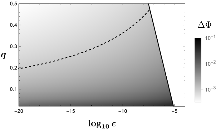
Finally, the bounds set so far on the mass and on can be used to check under what conditions the third requirement (c) is met. The methodology used is that of the Fisher matrix formalism, which allows the calculation of the variance with which the value of a parameter can be determined from a given signal, given the sensitivity curve of a detector and the Fourier transform of the theoretical prediction of the gravitational wave. This formalism is extensively used to make predictions for how accurate (future) detectors will be able to measure observables ,Maggiore.
The formalism states that the Fisher matrix , defined as
| (IV.9) |
where is the power spectral density of the detector under consideration, leads to the covariance matrix ,
| (IV.10) |
in which each element is the covariance of two observables . In particular, the square root of the diagonal elements of the covariance matrix are the standard deviations of each of the observables , and are therefore a direct measure of the accuracy with which the detector will be able to determine their values.
In what follows, we apply the Fisher matrix formalism to calculate the relative errors , i.e. the ratio of the standard deviation of the phase shift and the phase shift itself, for a range of ECO-models and a range of mass-ratios of the binary system. The gravitational waveform used is given by
| (IV.11) |
in which the phase is given by (II.3), the phase shift due to the resonance is given by (II.19a), and we have taken to be the TaylorF2 approximant to 2.5 PN order, as given in approximant. This approximant allows for the two component masses to have spin (that are taken to be aligned with the orbital angular momentum), but otherwise models them as featureless point particles. The resulting spin-orbit coupling and spin-spin coupling, respectively, are taken into account to 2.5 PN and 2 PN order. This approximant excludes non-resonant tidal forces. Those effects have already been investigated in Cardoso:2017cfl and excluding them is not expected to change the order of magnitude estimations provided by the Fisher matrix formalism. In the Fisher calculations to follow, the relative error is calculated for the coalescence time , coalescence phase , chirp mass, dimensionless mass ratio, and the phase shift. The value for the amplitude in (IV.11) is fixed by the choice of SNR. The upper cut-off frequency of the Fisher matrix calculation is taken to be the frequency corresponding to the ISCO of , whereas the lower cut-off frequency is dependent on the gravitational wave detector under consideration.
The calculation is done for Einstein Telescope using the power spectral density as given in PSD_ET. A similar Fisher calculation was performed using the power spectral density of the Advanced LIGO network, but the results showed that the relative error of the phase shift was much larger than unity for all phase space considered, leading to the conclusion that the current generation detectors are not able to measure the ECO shift. This result is corroborated by a recent paper NikhefResonances in which the binary black hole systems of GWTC-1 were analysed for resonances, and none were found. The results below will therefore focus on the Einstein Telescope. As such, the lower cut-off frequency in the definition of the Fisher matrix is taken to be .
IV.3 Results
Figure 3 shows the results for the relative errors on the phase shift for binary systems in which only the heavier of the two compact objects undergoes the resonance and is given a fixed mass , while the companion compact object’s mass is varied via the mass ratio of the binary system. This is done for five different fixed values for the heavier compact object, .
We take the regions within the contour line of unit relative error to be measurable by the detector. For the different ECO masses () considered, we find that, for the phase space considered, the resonance takes place well before the merger.


Top: for different values of the mass of the ECO, with lower relative errors below the contour.
Bottom: as indicated on the contours, for an ECO of mass .
However, these results show that for the most likely events for the Einstein Telescope (SNR 400), the resonances will be undetectable. Nevertheless, for unique events (SNR 4000, or a luminosity distance of order Mpc), the ECO resonance shifts for binaries of sufficiently asymmetric masses might be detected. In that case, we find that the relative error of the phase shift is smaller than unity over many orders of magnitude of . This wide range of is expected based on the weak (logarithmic) dependence of the phase shift on this parameter. We find that the width of this range increases for decreasing value of the ECO mass, and for increasingly asymmetric mass ratios. We find small relative errors exactly in the parameter range for which the phase shift (IV.4) is large, namely for small mass ratios and relatively large values of . Moreover, it reaches a minimal value for a binary of a given mass ratio. This minimal relative error is reached at larger for increasing ECO mass.
Given these results, most notably the required small value for the mass ratio and the fact that the companion star is expected to have a mass , candidates of ECOs that could be detected by the Einstein Telescope should have a mass of several tens to a hundred solar masses as well as be close enough to supply the required high SNR.
We have tested the robustness of these results by changing the values of the dimensionless spins of the binary system and have found the order of magnitudes of the relative error to be largely independent of such changes. We have also tested the robustness to variations in the cut-off frequency, to account for the fact that the ISCO-frequency of rotating black holes is not at , as well as this only being a test-particle approximation. Over the expected range of such corrections to the merging frequency, described for instance in favata2011conservative, we find that the relative errors change by at most a factor of order , with relative errors decreasing for higher cut-offs and increasing for lower cut-offs. We therefore conclude that the results presented are representative.
V Outlook
We derived an expression for the phase shift due to a tidal resonance in the Newtonian limit for circular orbits and spinless components and tested it in a Fisher analysis for the specific model of a reflecting surface. We believe that the dependence on the distance from the horizon and mass ranges for which the phase shift is significant are a robust order of magnitude estimate, that is more generally applicable:
First, we have also performed Fisher matrix calculations including aligned component spins as well as varying cut-off frequencies and the outcomes agree to the same order of magnitude. We believe this gives a qualitative indication that a similar phase shift can play a similar role also when other complications such as eccentric orbits are taken into account. Nevertheless, based on our results, it would be interesting to perform a more detailed analysis for smaller mass ratio systems. In particular, it would be interesting to perform a study of the effects for EMRI systems with LISA-targeted wave-forms in the future.
Second, the toy model of purely reflecting boundary conditions near the horizon allows to have a particular value of the phase shift depending on a minimum of parameters, but the method is more generally valid. For other objects for which the Love numbers and QNMs scale with redshift in a similar way as for the surface and , we expect a similar outcome. In general however, the reflection coefficient of a compact object will be smaller than unity, and therefore the phase shift we derived is likely an upper bound on the effect caused by resonant excitation of the fundamental QNM in those models. It would be interesting to investigate more general models of compact objects and run a Fisher analysis including the QNMs and Love numbers as free parameters, instead of keeping them fixed by the relation to .
Third, we focused on resonant excitation of the fundamental quadrupolar frequency . Other modes can play a role as well but the value of the phase shift is maximal for the quadrupole modes . Higher multipoles give a smaller contribution to the phase shift, as was indicated in (IV.5).
The study of overtone numbers through our method of replacing the overlap integral would involve going beyond the low frequency limit, and include besides the Love numbers also other tidal constants appearing in the low-frequency expansion of the linear response. To do this confidently, it should be quantified how strongly the low-frequency expansion coefficients are dominated by the lowest lying modes. In first instance, this means scrutinizing the assumption we have made that the contribution of higher order modes to the Love number is negligible, mainly on the argument that this should give the correct order of magnitude. We leave that to future work.
Acknowledgements.
We thank Archisman Ghosh, Thomas Hertog, Tanja Hinderer, Anuradha Samajdar, Maarten van de Meent, Chris Van den Broeck for discussions, the organizers of the Dutch multimessenger astronomy in the 2030s for the stimulating atmosphere that started part of this work. R.T, K.F. and B.V. thank the University of Maastricht for hospitality. R.T. thanks Nikhef for hospitality during the initial stages of this work. This work makes use of the Black Hole Perturbation Toolkit. K.F. is Aspirant FWO-Vlaanderen (ZKD4846-ASP/18). B.V. was partially supported by the National Science Foundation of Belgium (FWO) grant G.001.12, the European Research Council grant no. ERC-2013-CoG 616732 HoloQosmos, the KU Leuven C1 grant ZKD1118 C16/16/005, the FWO Odysseus grant G0H9318N and the COST action CA16104. The work of RT is supported in part by by the European Research Council grant no. ERC 616732 – HoloQosmos, bijzonder onderzoeksfonds C16/16/005 – horizons in hoge-energie fysica and COST Action CA16104 GWVerse. This paper is dedicated to the memory of Frederik Goelen, former PhD student at KU Leuven and contributor to the early stages of this work.Appendix A Low frequency expansions for BH perturbations
In Section III, we have given the expression (III.23) which relates, in the low frequency limit , a near-zone characterization of an ECO in terms of to the EFT characterization in terms of a tidal response function . In this appendix we will elucidate the derivation of this result. Our starting point is (III.20). To make this more explicit we first of all use the appropriate expansions for and from which one can derive, and . We find these expressions combining
| (A.1) |
| (A.2) |
where
| (A.3) |
| (A.4) |
from poisson1995 with
| (A.5) |
| (A.6) |
For the reflection and transmission coefficients one then finds
| (A.7) |
| (A.8) |
To find , we use from Chakrabarti2013
| (A.9) |
with
| (A.10) |
| (A.11) |
Here, the coefficients satisfy the recurrence relation
| (A.12) |
with
| (A.13) | |||||
| (A.14) | |||||
| (A.15) |
As is also stressed Chakrabarti2013, the limit becomes subtle due to poles in the -functions. One finds a different limit keeping generic and only setting after the expansion compared to starting with . To get consistent results, we follow the approach from Chakrabarti2013 which is to only let after the expansion. It should be noted however that, in any case, many of the intermediate results in Chakrabarti2013, including (III.19), are regularization dependent. Therefore, it is not entirely surprising that we will find a mismatch in coefficients with the post-Newtonian result by naively combining these results. It would be interesting to redo the analysis more consistently and explore how dynamic tidal effects can be resummed in a post-Newtonian expansion but, as this is not our main goal, we postpone it to future work.
The renormalized angular momentum ensures that the minimal solutions for and are compatible and is given in the low frequency expansion by Chakrabarti2013
| (A.16) |
Now from
| (A.17) |
one finds
| (A.18) |
We can continue, as Chakrabarti2013, by simply dropping the divergent term for as a type of ’minimal subtraction’. However, even if we expect this might capture the right functional form, it will not give the correct prefactor. In the main text we therefore leave this constant arbitrary, to be fixed by comparison with a post-Newtonian expansion. Nevertheless, continuing with the ’minimal subtraction’, for
| (A.19) |
and we finally find (III.23)
| (A.20) |
Appendix B From overlap integrals to Love numbers
We discuss the relation of the tidal constants to the overlap integrals in the Newtonian limit, adapted from Chakrabarti2013_1306.
The multipoles of the mass distribution, now called in the STF basis, are no longer independent variables but are given in terms of the mode amplitudes and overlap integrals as (cf. equation (4.9) in Chakrabarti2013_1306)
| (B.1) |
The effective action constructed in Chakrabarti2013_1306 leads to the linear response
| (B.2) |
where denotes Fourier transform. Equating those last two expressions for and using the solution to the harmonic oscillator equation (II.5) and (II.7), gives the linear response function:
| (B.3) |
Note that for the quadrupole such a pole expansion also holds beyond Newtonian limit Chakrabarti2013_1306, Chakrabarti2013.
The tidal deformability parameters are defined by the low frequency expansion of the response function
| (B.4) |
where is the tidal deformability related to the (electric) dimensionless tidal Love number , relates to the damping, to the response beyond the adiabatic approximation, etc. Note that often the linear response is restricted to the first coefficient in the above Taylor expansion of the linear response function. However, this is only valid far away from resonance, when .
Equating the two expressions (B.3) as a low frequency expansion and (B.4) formally allows to extract the overlap integrals as functions of the set of Taylor coefficients
| (B.5) |
in particular, for the lowest Taylor coefficients, we have
| (B.6) |
The parameter of our interest is the tidal deformability which relates to the dimensionless tidal Love number66 6 The Love numbers are normalized with respect to the mass of the object as in Cardoso:2017cfl. This makes it applicable for objects without a well-defined radius as for instance a boson star. as
| (B.7) |
As mentioned before, we will restrict to fundamental modes on the assumption that the associated overlap integrals are dominant above the ones with . This implies that the sum in (B.5) can be truncated to only. Given this assumption, the overlap integrals can be expressed in terms of the Love numbers
| (B.8) |
and response function to lowest order in becomes .
References
- [1] M. S. Morris, K. S. Thorne, and U. Yurtsever, “Wormholes, time machines, and the weak energy condition,” Phys. Rev. Lett. 61 (Sep, 1988) 1446–1449.
- [2] P. O. Mazur and E. Mottola, “Gravitational condensate stars: An alternative to black holes,” arXiv:gr-qc/0109035 [gr-qc].
- [3] F. E. Schunck and E. W. Mielke, “General relativistic boson stars,” Class. Quant. Grav. 20 (2003) R301–R356, arXiv:0801.0307 [astro-ph].
- [4] S. D. Mathur, “The Fuzzball proposal for black holes: An Elementary review,” Fortsch. Phys. 53 (2005) 793–827, arXiv:hep-th/0502050 [hep-th].
- [5] C. Barcelo, S. Liberati, S. Sonego, and M. Visser, “Fate of gravitational collapse in semiclassical gravity,” Phys. Rev. D77 (2008) 044032, arXiv:0712.1130 [gr-qc].
- [6] C. Barcelo, L. J. Garay, and G. Jannes, “Quantum Non-Gravity and Stellar Collapse,” Found. Phys. 41 (2011) 1532–1541, arXiv:1002.4651 [gr-qc].
- [7] C. Barcelo, R. Carballo-Rubio, L. J. Garay, and G. Jannes, “The lifetime problem of evaporating black holes: mutiny or resignation,” Class. Quant. Grav. 32 no. 3, (2015) 035012, arXiv:1409.1501 [gr-qc].
- [8] B. Holdom and J. Ren, “Not quite a black hole,” Phys. Rev. D95 no. 8, (2017) 084034, arXiv:1612.04889 [gr-qc].
- [9] G. Raposo, P. Pani, and R. Emparan, “Exotic compact objects with soft hair,” Phys. Rev. D99 no. 10, (2019) 104050, arXiv:1812.07615 [gr-qc].
- [10] S. L. Liebling and C. Palenzuela, “Dynamical Boson Stars,” Living Rev. Rel. 15 (2012) 6, arXiv:1202.5809 [gr-qc]. [Living Rev. Rel.20,no.1,5(2017)].
- [11] V. Cardoso and P. Pani, “Testing the nature of dark compact objects: a status report,” Living Rev. Rel. 22 no. 1, (2019) 4, arXiv:1904.05363 [gr-qc].
- [12] E. Seidel and W.-M. Suen, “Oscillating soliton stars,” Phys. Rev. Lett. 66 (Apr, 1991) 1659–1662.
- [13] M. Gleiser, “Pseudostable bubbles,” Phys. Rev. D49 (1994) 2978–2981, arXiv:hep-ph/9308279 [hep-ph].
- [14] E. Seidel and W.-M. Suen, “Formation of solitonic stars through gravitational cooling,” Phys. Rev. Lett. 72 (1994) 2516–2519, arXiv:gr-qc/9309015 [gr-qc].
- [15] V. Cardoso, E. Franzin, and P. Pani, “Is the gravitational-wave ringdown a probe of the event horizon?” Phys. Rev. Lett. 116 (Apr, 2016) 171101.
- [16] V. Cardoso, S. Hopper, C. F. B. Macedo, C. Palenzuela, and P. Pani, “Gravitational-wave signatures of exotic compact objects and of quantum corrections at the horizon scale,” Phys. Rev. D 94 (Oct, 2016) 084031.
- [17] V. Cardoso and P. Pani, “Tests for the existence of black holes through gravitational wave echoes,” Nat. Astron. 1 no. 9, (2017) 586–591, arXiv:1709.01525 [gr-qc].
- [18] R. S. Conklin, B. Holdom, and J. Ren, “Gravitational wave echoes through new windows,” Phys. Rev. D98 no. 4, (2018) 044021, arXiv:1712.06517 [gr-qc].
- [19] Z. Mark, A. Zimmerman, S. M. Du, and Y. Chen, “A recipe for echoes from exotic compact objects,” Phys. Rev. D96 no. 8, (2017) 084002, arXiv:1706.06155 [gr-qc].
- [20] R. H. Price and G. Khanna, “Gravitational wave sources: reflections and echoes,” Class. Quant. Grav. 34 no. 22, (2017) 225005, arXiv:1702.04833 [gr-qc].
- [21] Y.-T. Wang, Z.-P. Li, J. Zhang, S.-Y. Zhou, and Y.-S. Piao, “Are gravitational wave ringdown echoes always equal-interval?,” Eur. Phys. J. C 78 no. 6, (2018) 482, arXiv:1802.02003 [gr-qc].
- [22] Y.-T. Wang, J. Zhang, S.-Y. Zhou, and Y.-S. Piao, “On echo intervals in gravitational wave echo analysis,” Eur. Phys. J. C 79 no. 9, (2019) 726, arXiv:1904.00212 [gr-qc].
- [23] P. Bueno, P. A. Cano, F. Goelen, T. Hertog, and B. Vercnocke, “Echoes of Kerr-like wormholes,” Phys. Rev. D97 no. 2, (2018) 024040, arXiv:1711.00391 [gr-qc].
- [24] G. Ashton, O. Birnholtz, M. Cabero, C. Capano, T. Dent, B. Krishnan, G. D. Meadors, A. B. Nielsen, A. Nitz, and J. Westerweck, “Comments on: "Echoes from the abyss: Evidence for Planck-scale structure at black hole horizons",” arXiv:1612.05625 [gr-qc].
- [25] E. Maggio, A. Testa, S. Bhagwat, and P. Pani, “Analytical model for gravitational-wave echoes from spinning remnants,” Phys. Rev. D 100 no. 6, (2019) 064056, arXiv:1907.03091 [gr-qc].
- [26] J. Abedi, H. Dykaar, and N. Afshordi, “Echoes from the Abyss: Tentative evidence for Planck-scale structure at black hole horizons,” Phys. Rev. D96 no. 8, (2017) 082004, arXiv:1612.00266 [gr-qc].
- [27] J. Abedi, H. Dykaar, and N. Afshordi, “Echoes from the Abyss: The Holiday Edition!,” arXiv:1701.03485 [gr-qc].
- [28] N. Uchikata, H. Nakano, T. Narikawa, N. Sago, H. Tagoshi, and T. Tanaka, “Searching for black hole echoes from the LIGO-Virgo Catalog GWTC-1,” Phys. Rev. D100 no. 6, (2019) 062006, arXiv:1906.00838 [gr-qc].
- [29] R. K. L. Lo, T. G. F. Li, and A. J. Weinstein, “Template-based Gravitational-Wave Echoes Search Using Bayesian Model Selection,” Phys. Rev. D99 no. 8, (2019) 084052, arXiv:1811.07431 [gr-qc].
- [30] A. B. Nielsen, C. D. Capano, O. Birnholtz, and J. Westerweck, “Parameter estimation and statistical significance of echoes following black hole signals in the first Advanced LIGO observing run,” Phys. Rev. D99 no. 10, (2019) 104012, arXiv:1811.04904 [gr-qc].
- [31] A. Testa and P. Pani, “Analytical template for gravitational-wave echoes: signal characterization and prospects of detection with current and future interferometers,” Phys. Rev. D98 no. 4, (2018) 044018, arXiv:1806.04253 [gr-qc].
- [32] K. W. Tsang, M. Rollier, A. Ghosh, A. Samajdar, M. Agathos, K. Chatziioannou, V. Cardoso, G. Khanna, and C. Van Den Broeck, “A morphology-independent data analysis method for detecting and characterizing gravitational wave echoes,” Phys. Rev. D98 no. 2, (2018) 024023, arXiv:1804.04877 [gr-qc].
- [33] J. Westerweck, A. Nielsen, O. Fischer-Birnholtz, M. Cabero, C. Capano, T. Dent, B. Krishnan, G. Meadors, and A. H. Nitz, “Low significance of evidence for black hole echoes in gravitational wave data,” Phys. Rev. D97 no. 12, (2018) 124037, arXiv:1712.09966 [gr-qc].
- [34] V. Cardoso, E. Franzin, A. Maselli, P. Pani, and G. Raposo, “Testing strong-field gravity with tidal Love numbers,” Phys. Rev. D95 no. 8, (2017) 084014, arXiv:1701.01116 [gr-qc]. [Addendum: Phys. Rev.D95,no.8,089901(2017)].
- [35] A. Maselli, P. Pani, V. Cardoso, T. Abdelsalhin, L. Gualtieri, and V. Ferrari, “Probing Planckian corrections at the horizon scale with LISA binaries,” Phys. Rev. Lett. 120 no. 8, (2018) 081101, arXiv:1703.10612 [gr-qc].
- [36] N. K. Johnson-Mcdaniel, A. Mukherjee, R. Kashyap, P. Ajith, W. Del Pozzo, and S. Vitale, “Constraining black hole mimickers with gravitational wave observations,” arXiv:1804.08026 [gr-qc].
- [37] A. Maselli, P. Pani, V. Cardoso, T. Abdelsalhin, L. Gualtieri, and V. Ferrari, “From micro to macro and back: probing near-horizon quantum structures with gravitational waves,” Class. Quant. Grav. 36 no. 16, (2019) 167001, arXiv:1811.03689 [gr-qc].
- [38] S. Datta, R. Brito, S. Bose, P. Pani, and S. A. Hughes, “Tidal heating as a discriminator for horizons in extreme mass ratio inspirals,” Phys. Rev. D101 no. 4, (2020) 044004, arXiv:1910.07841 [gr-qc].
- [39] S. Datta, K. S. Phukon, and S. Bose, “Recognizing black holes in gravitational-wave observations: Telling apart impostors in mass-gap binaries,” arXiv:2004.05974 [gr-qc].
- [40] P. Pani, E. Berti, V. Cardoso, Y. Chen, and R. Norte, “Gravitational-wave signatures of the absence of an event horizon. II. Extreme mass ratio inspirals in the spacetime of a thin-shell gravastar,” Phys. Rev. D81 (2010) 084011, arXiv:1001.3031 [gr-qc].
- [41] V. Cardoso, A. del Rio, and M. Kimura, “Distinguishing black holes from horizonless objects through the excitation of resonances during inspiral,” Phys. Rev. D 100 (2019) 084046, arXiv:1907.01561 [gr-qc]. [Erratum: Phys.Rev.D 101, 069902 (2020)].
- [42] J. A. Pons, E. Berti, L. Gualtieri, G. Miniutti, and V. Ferrari, “Gravitational signals emitted by a point mass orbiting a neutron star: Effects of stellar structure,” Phys. Rev. D 65 (May, 2002) 104021.
- [43] L. Gualtieri, E. Berti, J. A. Pons, G. Miniutti, and V. Ferrari, “Gravitational signals emitted by a point mass orbiting a neutron star: A perturbative approach,” Phys. Rev. D 64 (Oct, 2001) 104007.
- [44] E. E. Flanagan and E. Racine, “Gravitomagnetic resonant excitation of rossby modes in coalescing neutron star binaries,” Phys. Rev. D 75 (Feb, 2007) 044001, arXiv:0601029 [gr-qc].
- [45] V. Cardoso, E. Franzin, A. Maselli, P. Pani, and G. Raposo, “Testing strong-field gravity with tidal love numbers,” Phys. Rev. D 95 (Apr, 2017) 084014.
- [46] T. Binnington and E. Poisson, “Relativistic theory of tidal love numbers,” Phys. Rev. D 80 (Oct, 2009) 084018.
- [47] É. É. Flanagan and T. Hinderer, “Constraining neutron-star tidal love numbers with gravitational-wave detectors,” Physical Review D 77 no. 2, (2008) 021502.
- [48] T. Damour and A. Nagar, “Relativistic tidal properties of neutron stars,” Phys. Rev. D 80 (Oct, 2009) 084035.
- [49] S. Datta and S. Bose, “Probing the nature of central objects in extreme-mass-ratio inspirals with gravitational waves,” Phys. Rev. D 99 no. 8, (2019) 084001, arXiv:1902.01723 [gr-qc].
- [50] J. Ruoff, P. Laguna, and J. Pullin, “Excitation of neutron star oscillations by an orbiting particle,” Phys. Rev. D63 (2001) 064019, arXiv:0005002 [gr-qc].
- [51] K. D. Kokkotas and G. Schaefer, “Tidal and tidal resonant effects in coalescing binaries,” Mon. Not. Roy. Astron. Soc. 275 (1995) 301, arXiv:9502034 [gr-qc].
- [52] Y. Kojima, “Stellar Resonant Oscillations Coupled to Gravitational Waves,” Progress of Theoretical Physics 77 no. 2, (02, 1987) 297–309.
- [53] A. Reisenegger and P. Goldreich, “Excitation of neutron star normal modes during binary inspiral,” Astrophysical Journal 426 (06, 1994) .
- [54] D. Lai, “Resonant oscillations and tidal heating in coalescing binary neutron stars,” Mon. Not. Roy. Astron. Soc. 270 (1994) 611, arXiv:9404062 [astro-ph].
- [55] Y. Rathore, R. D. Blandford, and A. E. Broderick, “Resonant excitation of white dwarf oscillations in compact object binaries. 1. The No back reaction approximation,” Mon. Not. Roy. Astron. Soc. 357 (2005) 834, arXiv:astro-ph/0406102 [astro-ph].
- [56] C. F. B. Macedo, P. Pani, V. Cardoso, and L. C. B. Crispino, “Astrophysical signatures of boson stars: quasinormal modes and inspiral resonances,” Phys. Rev. D 88 no. 6, (2013) 064046, arXiv:1307.4812 [gr-qc].
- [57] Asali, Pang, Samajdar, Van Den Broeck, “Probing resonant excitations in exotic compact objects via gravitational waves,” arXiv:gr-qc/2004.05128 [gr-qc].
- [58] W. D. Goldberger and I. Z. Rothstein, “An Effective field theory of gravity for extended objects,” Phys. Rev. D73 (2006) 104029, arXiv:0409156 [hep-th].
- [59] S. Chakrabarti, T. Delsate, and J. Steinhoff, “Effective action and linear response of compact objects in Newtonian gravity,” Phys. Rev. D88 (2013) 084038, arXiv:1306.5820 [gr-qc].
- [60] S. Chakrabarti, T. Delsate, and J. Steinhoff, “New perspectives on neutron star and black hole spectroscopy and dynamic tides,” arXiv:1304.2228 [gr-qc].
- [61] J. Steinhoff, T. Hinderer, A. Buonanno, and A. Taracchini, “Dynamical Tides in General Relativity: Effective Action and Effective-One-Body Hamiltonian,” Phys. Rev. D 94 no. 10, (2016) 104028, arXiv:1608.01907 [gr-qc].
- [62] P. Pani, L. Gualtieri, T. Abdelsalhin, and X. Jiménez-Forteza, “Magnetic tidal Love numbers clarified,” Phys. Rev. D 98 no. 12, (2018) 124023, arXiv:1810.01094 [gr-qc].
- [63] T. Hinderer, “Tidal Love numbers of neutron stars,” Astrophys. J. 677 (2008) 1216–1220, arXiv:0711.2420 [astro-ph].
- [64] T. Regge and J. A. Wheeler, “Stability of a schwarzschild singularity,” Physical Review 108 no. 4, (1957) 1063.
- [65] K. Martel and E. Poisson, “Gravitational perturbations of the Schwarzschild spacetime: A Practical covariant and gauge-invariant formalism,” Phys. Rev. D 71 (2005) 104003, arXiv:gr-qc/0502028.
- [66] S. Chandrasekhar, “On the equations governing the perturbations of the schwarzschild black hole,” Proceedings of the Royal Society of London. A. Mathematical and Physical Sciences 343 no. 1634, (1975) 289–298.
- [67] S. H. Völkel and K. D. Kokkotas, “Ultra Compact Stars: Reconstructing the Perturbation Potential,” Class. Quant. Grav. 34 no. 17, (2017) 175015, arXiv:1704.07517 [gr-qc].
- [68] N. Loutrel and N. Yunes, “Eccentric Gravitational Wave Bursts in the Post-Newtonian Formalism,” Class. Quant. Grav. 34 no. 13, (2017) 135011, arXiv:1702.01818 [gr-qc].
- [69] Z. Nasipak, T. Osburn, and C. R. Evans, “Repeated faint quasinormal bursts in extreme-mass-ratio inspiral waveforms: Evidence from frequency-domain scalar self-force calculations on generic Kerr orbits,” Phys. Rev. D 100 no. 6, (2019) 064008, arXiv:1905.13237 [gr-qc].
- [70] B. C. Mundim, H. Nakano, N. Yunes, M. Campanelli, S. C. Noble, and Y. Zlochower, “Approximate black hole binary spacetime via asymptotic matching,” Phys. Rev. D 89 no. 8, (2014) 084008, arXiv:1312.6731 [gr-qc].
- [71] M. Sasaki and H. Tagoshi, “Analytic black hole perturbation approach to gravitational radiation,” Living Rev. Rel. 6 (2003) 6, arXiv:gr-qc/0306120.
- [72] E. Poisson and M. Sasaki, “Gravitational radiation from a particle in circular orbit around a black hole. 5: Black hole absorption and tail corrections,” Phys. Rev. D 51 (1995) 5753–5767, arXiv:gr-qc/9412027.
- [73] J. M. Bardeen and W. H. Press, “Radiation fields in the schwarzschild background,” Journal of Mathematical Physics 14 no. 1, (1973) 7–19.
- [74] S. A. Teukolsky, “Perturbations of a rotating black hole. 1. Fundamental equations for gravitational electromagnetic and neutrino field perturbations,” Astrophys. J. 185 (1973) 635–647.
- [75] S. Isoyama, R. F. P. Mendes, and E. Poisson, “Self-force and fluid resonances,” Class. Quant. Grav. 33 no. 8, (2016) 085002, arXiv:1512.00059 [gr-qc].
- [76] T. D. Drivas and S. E. Gralla, “Dependence of Self-force on Central Object,” Class. Quant. Grav. 28 (2011) 145025, arXiv:1009.0504 [gr-qc].
- [77] V. Cardoso and P. Pani, “The observational evidence for horizons: from echoes to precision gravitational-wave physics,” arXiv:1707.03021 [gr-qc].
- [78] Maggiore, M., “Gravitational Waves, Volume 1: Theory and Experiments,” Oxford University Press, ISBN 978-0-19-857074-5.
- [79] Arun, Buonanno, Faye, Ochsner, “Higher-order spin effects in the amplitude and phase of gravitational waveforms emitted by inspiraling compact binaries: Ready-to-use gravitational waveforms,” Phys. Rev. D 79 (2009) , arXiv:gr-qc/0810.5336 [gr-qc].
- [80] http://www.et-gw.eu/index.php/etsensitivities#datafiles.
- [81] M. Favata, “Conservative corrections to the innermost stable circular orbit (isco) of a kerr black hole: A new gauge-invariant post-newtonian isco condition, and the isco shift due to test-particle spin and the gravitational self-force,” Physical Review D 83 no. 2, (2011) 024028.