Hyperbolic Discretization via Riemann Invariants
Abstract
We are interested in numerical schemes for the simulation of large scale gas networks. Typical models are based on the isentropic Euler equations with realistic gas constant. The numerical scheme is based on transformation of conservative variables in Riemann invariants and its corresponding numerical dsicretization. A particular, novelty of the proposed method is the possbility to allow for an efficient discretization of the boundary and coupling conditions at nodal points of the network. The original discretization is analysed in view of its property to correctly recover steady states as well as to resolve possible analytic solutions. Comparisons with existing methods show the advantage of the novel method.
1 Introduction
Mathematical models for transport of high–pressure natural gas through a pipeline system has been subject of active research both in engineering literature e.g. [28, 33, 34, 2, 1] as well as in mathematical literature, see e.g. [5, 6, 26, 25, 9, 12, 29, 23, 17] and the references therein. Depending on the application and physical regimes different mathematical descriptions can be used for transport in pipe systems. This leads to a hierarchy of models available and we refer e.g. to [25, 30] for further details. Besides the mathematical models for the gas flow in the pipe different conditions for coupling the flow at pipe–to–pipe intersections have been proposed and we refer to [5, 6, 29] for modeling aspects as well as to [14, 13, 11] for well–posedness results.
In high–pressure and long–distance pipelines typical pressure mass flux suggests to neglect inertia and gravity effects in the mathematical model [25, 9, 34] . Those models are also called friction dominated models and they can be obtained through asymptotic analysis. They are independent of temperature. The governing equations are given by
| (1) |
Here, denotes the gas density at time and position where and is the length of the pipe. The factor is the friction factor and the diameter of the pipe. The gas velocity is denoted by and the pressure by .The previous equation is not closed and density–pressure relation referred to as pressure law needs to be prescribed. For isentropic Euler equations the relation is given by and the value of for ideal gas is Below we discuss further choices in detail. If inertia effects are accounted for, equation (1) reads
| (2) |
Recently, the mathematical discussion has been extended to nonlinear hyperbolic models for gas flows using generalized pressure laws of the type
| (3) |
The function is called compressibility factor. In [15] different compressibility factors (3) have been compared, both analytically and by data obtained of measurements of a natural gas pipeline. Therein, a factor
| (4) |
for some has been proposed. Classical solutions to the isentropic Euler equations (2) and the pressure law (4) has been analysed in detail in [24]. Also, steady states of this system have been analysed in [23]. In this work we focus on a suitable numerical discretization of equation (5) in the presence of general compressibility factors (3) and a numerical formulation suitable to treat gas networks.
In [4] it has been argued that for a semilinear model can be derived. This is obtained by neglecting the term but retain In the case of given by the isothermal Euler equations, i.e., the obtained model (2) is a linear wave equation. In the case of a generalized pressure law (3) the model is given by
| (5) |
2 Qualitative Properties of Model (5)
Prior to the numerical discretization we discuss some properties. Assuming that , the system (6) enjoys similar properties as the system in Lagrangian coordinates. Therefore, we do not repeat a discussion of its properties but only state the properties relevant for the numerical scheme later on. In the following we consider the function which is implicitly defined by Further, we discuss properties in terms of the conservative variables The Jacobian of the flux function is given by with . The eigenvalues are
| (7) |
To obtain strict hyperbolicity we impose the assumption
| (8) |
The assumption (8) is fulfilled if we assume . Note that in the case of the isentropic Euler equations and for a pressure law of the type (4) the assumption (8) is fulfilled. (Right) eigenvectors to the eigenvalues are , respectively. Both characteristic fields are genuine nonlinear provided that Note that in the case of isothermal Euler equations () the fields are linearly degenerated. As noted before system (5) reduces to a linear wave equation. In the case of the pressure law (4) the condition is fulfilled due to the assumption of strictly hyperbolicity.
Since under Assumption (8) we have
| (9) |
Provided (8) holds true, the system is a hyperbolic balance law and therefore two Riemann invariants exists, in the following denoted by and given by
| (10) |
The Riemann invariants are transported with speed i.e., fulfills
| (11) |
Here, and are density and velocity obtained by inverting equation (10). The precise formulas will be given below. Under the assumption 8 , with we have
| (12) |
and for smooth solutions the values are transported along characteristics with slope respectively. Also, shocks (or contact discontinuities in the case ) are not observed under typical gas operational conditions [4, 25, 24]. The equations (11) are in non–conservative form. It is therefore not well–defined in the case of discontinuous However, this form exhibits the transport nature of the problem and we propose a numerical discretization related to the transport character of equation (11) for sufficiently smooth solutions. This discretization allows to identify correct boundary conditions that may not be obtained in the case of applying a central discretization schemes towards the conservative formulation of the problem.
Finally, we note that equation (6) allows for explicit solutions that can be used for validation of the numerical scheme. The solutions are found similarly to the approach in [23]: Let be any positive constant. Then, is a solution to equation (6). Indeed, is constant and implies is independent of Therefore, conservation of mass holds true. Furthermore,
| (13) |
and therefore the conservation of momentum is satisfied for and postive . We have and if , then for and is a solution. is a degree of freedom in the solution that can be used to match possible boundary conditions.
In [22] traveling wave solutions to equation (2) and (4) have been studied. For equation (6) we can proceed in a similar fashion. Consider a pressure law of the type (4) with Then, we obtain an equation for the pressure as follows
| (14) |
A traveling wave solution is of type For any of this type we have by definition provided that With and , we obtain conservation of mass
| (15) |
An equation for is obtained from the momentum equation. Written in terms of and for it reads
| (16) |
Its explicit solution fulfills and therefore a closed form using Lambert–W function can be given.
3 Numerical Discretization
To derive the scheme we consider the system (6) in a single pipe. The pipe is paramterized by and we assume (8) holds true. The spatial domain is discretized in equidistant intervals of size The center of each cell is denoted by , and we assume is such that We are interested in a discretization for based on a discretization of the formulation in Riemann invariants. For the Riemann invariants are given by
| (17) |
where We further denote by and Assuming sufficiently smooth solutions equation (11) will be discretized using a first–order finite–volume scheme. We denote the local cell average in cell as by
| (18) |
The piecewise constant reconstruction by cell with cell average is denoted by i.e., For simplicity of notation we still use computed using Riemann invariants . Integration yields
| (19) |
Within cell we use a constant reconstruction of the functions and by the cell averages The corresponding cell average is denoted by for Approximating and a midpoint rule to the source term we obtain up to order
| (20) |
Due to assumption (12) we use an Upwind discretization. This implies that since we approximate for and similarly since we approximate This leads to the following discretization for
| (21) | ||||
| (22) |
Any explicit temporal discretization on with time step has to fulfill the CFL condition
| (23) |
Equations (21) and (22) require boundary conditions for at and boundary conditions for at respectively.
Discretization in conservative variables
The numerical scheme (21) and (22) is reformulated in terms of cell averages of conservative variables Further, we denote by
| (24) |
and we have We compute
| (25) | ||||
| (26) | ||||
| (27) | ||||
| (28) |
and similarly
| (29) | ||||
| (30) | ||||
| (31) |
Hence, a semi–discretization for the cell averages in conservative variables is given by
| (32) | ||||
| (33) |
where and and using (9) and . The previous equation has to be complemented with suitable boundary conditions obtained by equation (21) for and by equation (22) for i.e.,
| (34) |
Using equation (9) those equations allow to derive boundary conditions for , :
| (35) | ||||
| (36) |
Additionaly, we assume initial conditions and boundary conditions given:
| (37) |
For a single pipe we therefore obtain the following semi–discretized system together with discretized initial and boundary conditions
| (38) | ||||
| (39) | ||||
| (40) | ||||
| (41) | ||||
| (42) |
Other discretization schemes
In the numerical experiments we compare this discretization against others from the literature. The first one is given in [21] and uses a midpoint discretization:
| (43) | ||||
| (44) | ||||
| (45) |
Another one can be found in [20, 31] and will be called endpoint discretization in the following:
| (46) | ||||
| (47) | ||||
| (48) |
Consistent discretization of steady–states
Schemes that preserve steady states exactly are called well-balanced, and their development is a lively topic in the field of hyperbolic balance laws, see e.g. [19, 3, 8, 27, 10, 32] and references therein. Usually, these schemes use specific knowledge of an equilibrium state. For the proposed scheme and in the case we obtain the following results: The proposed scheme conserves the continuous steady state at most to order and the scheme conserves discrete steady states exactly.
Provided for some constant Then, the continuous steady state of the system (5) are
| (49) |
where we recall If we assume that the data is given by equation (49) then, the discretized steady states are at the cell center are given by
| (50) |
Applying the previous scheme with initial conditions given by equation (50) yields
| (51) | ||||
| (52) |
By definition we have and therefore the last equation is equal to zero up to the order Hence, and the scheme approximates the continuous steady state up to order Clearly, it is possible to define higher–order integration of the source term, e.g., replacing by where are integration weights and with By the proposed Upwind scheme it is not reasonable to have stencils beyond and for the integration of the source term. This leaves as integration schemes Newton-Cotes formulas. With three points we may use Simpson’s formula with an error of This yields consistency in this case up to order if we discretize
| (53) |
We also consider the conservation of discrete steady statesfor the same choice of Then, and the discretization simplifies to
| (54) |
Consider an explicit Euler discretization as temporal discretization and denote by Assume that for all at time and Those are the discrete steady states of the scheme (54). Then, an explicit Euler discretization yields
| (55) |
Therefore, the scheme preserves the discrete steady states exactly for all future times
Discretization of pipe networks
A pipe networks is modelled as directed graph where is the set of all edges and the set of all vertices. For the vertices we distinguish between internal nodes in the network (having a degree larger or equal to two) and boundary nodes of the network, i.e., vertices with degree one. For vertices of degree equal to one we may either prescribe pressure or mass flux conditions as in equation (42). For the internal nodes we use coupling conditions given by equal pressure and the conservation of mass (60). For further details and a discussion of the coupling conditions we refer to [28, 5] and references therein.
We introduce the following notation. For simplicity we assume all pipes are parameterized by . By we denote the cell average of the pressure and mass flux in pipe and cell of pipe at time Hence, the equations for the temporal evolution of the cell averages and are then given by equations
| (56) | ||||
| (57) | ||||
| (58) | ||||
| (59) |
and initial conditions. For a vertex denote the set of all edges incoming to by and all edges exiting from by In case the coupling conditions at the vertex
| (60) |
Conditions (60) together with intial conditions, boundary conditions for pressure and mass flux at nodes of degree one and the discretization on the network form the fully discrete scheme. Let be a vector stacking all discretization points of all pipes of the pressure in one vector and the same for all mass fluxes in . The only points not included as they are already known are the start and end nodes which have prescribed boundary conditions. Then equation (56)-(59) can be written as
| (61) |
where and are the pressure and mass flux boundary conditions. Adding equation (60) into that the full equation reads
| (62) |
4 Computational Results
In the following we consider three networks: a pipe, the diamond benchmark also described in [7] and a realistic network mentioned in [18]. The networks and the numerical simulations are described in the following sections.
4.1 Simulation of Gas Flow in a Single Pipe
The pipe is 3 km long and has a diameter of 0.762m and a friction factor and . We compare the new discretization with the two other discretizations mentioned before, one which we call midpoint discretization and abbreviated by “mid” and an endpoint discretization abbreviated by “end”. In particular, consider two scenarios shown in Figure 1 and 2. In the first scenario we start the system in a stationary solution and then abruptly decrease the pressure at the inlet of the pipe. We compute the pressure at the outlet and the flux at the inlet which then dynamically changes until the system goes back to a stationary solution. The flux at the outlet is kept constant. The three different results for different discretization schemes are plotted in Figure 1, and we observe that the novel discretization does not lead to any oscillations in flux and pressure. The discretization ‘mid’ produces unphysical oscillations.
In the second scenario we change the flux every 1000 seconds according to Figure 2 by keeping a constant pressure at the inlet of 75 bar. This yields a change of the mass flow at the inlet and a change of the pressure at the outlet. Since the dynamic behaviour is not recognizable over this long time period all numerical schemes give basically the same result.
In Table 1 we summarize the simulation time for the two scenarios named “step” and “wave” and the three different methods. Here we see that the novel method outperforms the other methods. The time is wall time and we use ode15s a MATLAB ODE solver, which can handle index–1 DAEs to do the time integration.
| method | step | wave |
|---|---|---|
| end | 0.45 | |
| mid | 3.98 | |
| new | 0.28 |
4.2 Resolution of Steady States
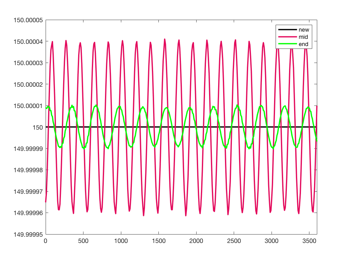
If the boundary conditions are kept contant in time the system will converge to steady state. This is true for all three discretizations. However the steady state of the new discretization is the only state which is actually steady. While the other numerical states are states that yields fluctuations around the constant steady state. For our next numerical experiment we again simulated on a pipe of length 3km, with a diameter of 0.762m and a friction factor and . We put a pressure of 155 constant on the inlet of the pipe and a constant flux of 150 kg/s on the outlet of the pipe. The stationary solution is the given by a constant mass flux in the entire pipe of 150 kg/s and a pressure of bar. However for the endpoint and midpoint discretization we observe oscillations that do not decay over time as shown in Figure 3.
4.3 Simulation of a Diamond–shaped Network
The network consists of 9 pipes, all of length 1km, diameter of 1m and a friction factor . All nodes are at the same geodesic height and all pipes are flat. We use it to show how different the three discretization schemes resolve the dynamic behaviour.

In this scenario we keep the pressure at the inlet constant 70 bar and increase the mass flux at the outlet of the network, the demand node from 30 kg/s to 40 kg/s. We use a constant . In Figure 5 we see the very different restults in particular for the pressure at the supply node. Again as already seen for the simple pipe example the novel discretization does not generate unphysical oscillations.
4.4 Simulation of a Pipe Network
The new discretization is also used on a realistic network, whose topolgy is illustrated in Figure 6. Node 1 is a supply node and all the other nodes that are end nodes are demand nodes. This network has a total of 46 nodes with 1 supply nodes, 13 interior noes and 23 supply nodes. To keep it simple and reproducible the pipes are all 10 km long, 0.6 m wide and have a roughness of 0.01 resulting in a friction factor of 0.0454. Again is constant. We simulated a scenario where at the simple stationary point all fluxes are zero and all the pressures are identically 800 bar. This state is modified by a sudden increase at the outlet flux to 40 kg/s at all demand nodes. The pressure at two different outlets and the flux at the inlet is shown in Figure 7 for the new discretization and the endpoint discretization.

5 Conclusions
We showed that the discretization using Riemann invariants allows to correctly approximate the transport phenomena underlying the nonlinear model. The novel discretization does not lead to any oszillations when converging to steady state. It is also approximates the discrete steady state to any order. Numerical experiments show also for complex network geometries a good performance of the scheme. It also keeps all the advantages of the endpoint discretizations for the numerical treatment as a differential algebraic system and can be computed efficiently.
Acknowledgment
This work has been supported by HE5386/14,15-1, BMBF ENets 05M18PAA , BMWi mathenergy 0324019B, ERDF/EFRE: ZS/2016/04/78156 and ID390621612 Cluster of Excellence Internet of Production (IoP).
References
- [1] www.psig.org.
- [2] www.simone.eu.
- [3] E. Audusse, F. Bouchut, M.-O. Bristeau, R. Klein, and B. Perthame, A fast and stable well-balanced scheme with hydrostatic reconstruction for shallow water flows, SIAM J. Sci. Comput., 25 (2004), pp. 2050–2065.
- [4] P. Bales, O. Kolb, and J. Lang, Hierarchical modelling and model adaptivity for gas flow on networks, Computational Science – ICCS 2009, (2009), pp. 337–346.
- [5] M. K. Banda, M. Herty, and A. Klar, Coupling conditions for gas networks governed by the isothermal Euler equations, Netw. Heterog. Media, 1 (2006), pp. 295–314.
- [6] , Coupling conditions for gas networks governed by the isothermal Euler equations, Netw. Heterog. Media, 1 (2006), pp. 295–314 (electronic).
- [7] P. Benner, S. Grundel, C. Himpe, C. Huck, T. Streubel, and C. Tischendorf, Gas network benchmark models, in Differential-Algebraic Equations Forum, Springer, 2018, pp. 1–27. (Accepted).
- [8] A. Bollermann, G. Chen, A. Kurganov, and S. Noelle, A well-balanced reconstruction of wet/dry fronts for the shallow water equations, Journal of Scientific Computing, 56 (2013), pp. 267–290.
- [9] J. Brouwer, I. Gasser, and M. Herty, Gas pipeline models revisited: model hierarchies, nonisothermal models, and simulations of networks, Multiscale Model. Simul., 9 (2011), pp. 601–623.
- [10] A. Chertock, S. Cui, A. Kurganov, Ş. N. Özcan, and E. Tadmor, Well-balanced central-upwind schemes for the euler equations with gravitation, (2015). Submitted.
- [11] R. M. Colombo and M. Garavello, A well posed Riemann problem for the -system at a junction, Netw. Heterog. Media, 1 (2006), pp. 495–511.
- [12] R. M. Colombo, G. Guerra, M. Herty, and V. Schleper, Optimal control in networks of pipes and canals, SIAM J. Control Optim., 48 (2009), pp. 2032–2050.
- [13] R. M. Colombo, M. Herty, and V. Sachers, On conservation laws at a junction, SIAM J. Math. Anal., 40 (2008), pp. 605–622.
- [14] R. M. Colombo and C. Mauri, Euler system for compressible fluids at a junction, J. Hyperbolic Differ. Equ., 5 (2008), pp. 547–568.
- [15] J. C. de Almeida, J. A. Velásquez, and R. Barbieri, A methodology for calculating the natural gas compressibility factor for a distribution network, Petroleum Science and Technology, 32 (2014), pp. 2616–2624.
- [16] S. A. Dyachenko, A. Zlotnik, A. O. Korotkevich, and M. Chertkov, Operator splitting method for simulation of dynamic flows in natural gas pipeline networks, Physica D: Nonlinear Phenomena, 361 (2017), pp. 1–11.
- [17] H. Egger, A robust conservative mixed finite element method for isentropic compressible flow on pipe networks, SIAM J. Sci. Comput., 40 (2018), pp. A108–A129.
- [18] M. Farzaneh-Gord and H. R. Rahbari, Unsteady natural gas flow within pipeline network, an analytical approach, Journal of Natural Gas Science and Engineering, 28 (2016), pp. 397–409.
- [19] J. M. Greenberg and A. Y. Leroux, A well-balanced scheme for the numerical processing of source terms in hyperbolic equations, SIAM J. Numer. Anal., 33 (1996), pp. 1–16.
- [20] S. Grundel and L. Jansen, Efficient simulation of transient gas networks using IMEX integration schemes and MOR methods, in 54th IEEE Conference on Decision and Control (CDC), 2015, pp. 4579–4584.
- [21] S. Grundel, L. Jansen, N. Hornung, T. Clees, C. Tischendorf, and P. Benner, Model order reduction of differential algebraic equations arising from the simulation of gas transport networks, in Progress in Differential-Algebraic Equations, Differential-Algebraic Equations Forum, Springer, 2014, pp. 183–205.
- [22] M. Gugat, R. Schultz, and D. Wintergerst, Networks of pipelines for gas with nonconstant compressibility factor: stationary states, Computational and Applied Mathematics, 37 (2016), pp. 1066–1097.
- [23] M. Gugat and S. Ulbrich, The isothermal Euler equations for ideal gas with source term: product solutions, flow reversal and no blow up, J. Math. Anal. Appl., 454 (2017), pp. 439–452.
- [24] , Lipschitz solutions of initial boundary value problems for balance laws, Math. Models Methods Appl. Sci., 28 (2018), pp. 921–951.
- [25] M. Herty, J. Mohring, and V. Sachers, A new model for gas flow in pipe networks, Math. Methods Appl. Sci., 33 (2010), pp. 845–855.
- [26] O. Kolb, J. Lang, and P. Bales, An implicit box scheme for subsonic compressible flow with dissipative source term, Numer. Algorithms, 53 (2010), pp. 293–307.
- [27] S. Noelle, N. Pankratz, G. Puppo, and J. Natvig, Well-balanced finite volume schemes of arbitrary order of accuracy for shallow water flows, J. Comput. Phys., 213 (2006), pp. 474–499.
- [28] A. Osiadacz, Simulation and analysis of gas networks, Gulf Publishing Company, Houston, 1989.
- [29] G. A. Reigstad, Existence and uniqueness of solutions to the generalized Riemann problem for isentropic flow, SIAM J. Appl. Math., 75 (2015), pp. 679–702.
- [30] F. Rüffler, V. Mehrmann, and F. M. Hante, Optimal model switching for gas flow in pipe networks, Networks & Heterogeneous Media, 13 (2018), pp. 641–661.
- [31] J. J. Stolwijk and V. Mehrmann, Error analysis and model adaptivity for flows in gas networks, Analele Universitatii" Ovidius" Constanta-Seria Matematica, 26 (2018), pp. 231–266.
- [32] Y. Xing and C.-W. Shu, High order well-balanced WENO scheme for the gas dynamics equations under gravitational fields, J. Sci. Comput., 54 (2013), pp. 645–662.
- [33] A. Zlotnik, M. Chertkov, and S. Backhaus, Optimal control of transient flow in natural gas networks, in 2015 54th IEEE Conference on Decision and Control, IEEE, 2015.
- [34] A. Zlotnik, L. Roald, S. Backhaus, M. Chertkov, and G. Andersson, Coordinated scheduling for interdependent electric power and natural gas infrastructures, IEEE Transactions on Power Systems, 31 (2016).