The interval turnpike property for adjointsThanks: This work was supported by the DFG Grants GR 1569/17-1 and SCHI 1379/5-1 and was conducted while the third author was visiting University of Bayreuth under Academy of Finland Grant number 310489 held by Lassi Paunonen and supported by a travel grant from the Magnus Ehrnrooth Foundation.
Abstract.
In this work we derive an interval turnpike result for adjoints of finite- and infinite-dimensional nonlinear optimal control problems under the assumption of an interval turnpike on states and controls. We consider stabilizable dynamics governed by a generator of a semigroup with finite-dimensional unstable part satisfying a spectral decomposition condition and show the desired turnpike property under continuity assumptions on the first-order optimality conditions. We further give stronger estimates for analytic semigroups and provide a numerical example with a boundary controlled semilinear heat equation to illustrate the results.
Key words and phrases:
Turnpike property, optimal control, nonlinear systems, partial differential equations2010 Mathematics Subject Classification
93D20, 49K20, 49K40, 93B05, 93B071. Introduction
The turnpike property is a particular feature of optimal solutions of dynamic optimal control problems (OCPs). It is characterized by the phenomenon of optimal solutions to long-horizon OCPs staying close a specific steady state, the so-called turnpike, for the majority of the time. First described in a paper by von Neumann in the middle of the 20th century [27], turnpike behavior has since received vast interest, cf. the recent works [16, 18, 19, 20, 29, 32, 34, 38]. For nonlinear problems, a way to derive turnpike properties is linearization of the extremal equations, analysis of the linearization and a smallness assumption, cf. [4, 17, 35, 36]. Another possibility is to assume a particular notion of dissipativity, cf. [7, 9, 14, 15], which has the advantage to allow for global turnpike properties on state and control, i.e., without a smallness condition on, e.g., the initial distance to the turnpike. In that context, however, up to now there were no results on the behavior of the corresponding adjoints. Thus, in this paper, we will show that the turnpike behavior of state and control induces turnpike behavior of the adjoints without smallness assumptions. To this end, we analyze the first-order necessary optimality conditions and, loosely speaking, show for problems governed by general evolution equations that continuity of the nonlinearities and convergence of state and control imply convergence of the adjoints. While our results are formulated in an infinite-dimensional setting, the results are new also for finite-dimensional systems, which form a special case of our setting. Besides being an important structural property of the optimal triplet, turnpike properties can be leveraged in design of numerical methods. For example [36] suggests to exploit them in indirect shooting methods, in [16, 17] it is used for tailored discretization of infinite dimensional OCPs in a receding-horizon setting and [10] hinges on them in mixed-integer OCPs.
After introducing the optimal control problem, the first-order conditions and the functional analytic setting in Section 2, we deduce the desired turnpike property of the adjoints in Section 3 for exponentially stable and exactly controllable systems. Assuming that the underlying operator satisfies a spectrum decomposition assumption, we prove the result in Section 4 for stabilizable systems with finite-dimensional unstable part. In Section 5 we provide stronger estimates assuming more structure of the problem, i.e., that the underlying semigroup is analytic and hence the dynamics are given by a parabolic evolution equation. Further in Section 6 we discuss and give sufficient conditions for our main assumption, i.e., interval turnpike behavior of state and control. Finally in Section 7 we present a numerical example with a boundary controlled semilinear heat equation on a two-dimensional domain.
2. Setting and preliminaries
Let be a Banach space and be a Hilbert space with corresponding norm . Consider the optimal control problem
| (2.1) | ||||
where is sufficiently smooth, , generates a strongly continuous semigroup on , , and is a sufficiently smooth, locally Lipschitz nonlinearity. We will assume that the above problem has at least one optimal solution , cf. [24, Chap. 3]. Additionally, we consider to be an optimal solution of the corresponding steady state system, i.e., solves
| (2.2) | ||||
Our goal in this paper is to find conditions under which interval turnpike behavior of the states and control inputs implies interval turnpike behavior of the adjoints. Our basic assumption on the behavior of the optimal solutions is thus the following.
Assumption 2.1 (Interval turnpike property for states and controls).
We assume there are strictly monotonously increasing functions with such that is strictly monotonously increasing and unbounded and for each there is such that
Note that this bound immediately implies .
Remark 2.2.
We say that satisfies the exponential turnpike property, if there is a constant and a decay parameter , both independent of such that we have
If this inequality holds, it can be easily seen, cf. [18, Discussion after Rem. 6.3] that we can choose such that for each there is a horizon such that
and
i.e., and uniform convergence on a fixed part of the time interval for . Thus, 2.1 is satisfied with , and .
The corresponding necessary optimality conditions of above problem (2.1) read, cf. [24, Chap. 4],
| (2.3) | ||||
| where and . Analogously, the optimality conditions of the steady state problem read | ||||
Our goal in this paper is to show the interval turnpike property of the adjoint .
Definition 2.3 (Interval turnpike property for adjoint states).
We say that the adjoint satisfies the interval turnpike property at the steady state adjoint , if there are strictly monotonously increasing functions with such that is strictly monotonously increasing and unbounded and for each there is such that
For our analysis, we define the remainder terms
| and for | ||||
| Thus, denoting , , and , we have that | ||||
| (2.4) | ||||
| (2.5) | ||||
| (2.6) | ||||
with and . It is clear that the solutions , , and of eq. 2.3 depend on and hence also , , and do. However, for the sake of readability, we do not explicitly indicate this dependence. We note that, using the definition of , , and , the inequalities from Assumption 2.1 and Definition 2.3 can be written as and , respectively.
Remark 2.4 (Extension to box constraints on the control).
We briefly discuss how the case of box constraints on the control can be treated analogously to the unconstrained case, if one assumes that the turnpike lies in the interior of the constraints. To this end, in the dynamic problem (2.1) we add the constraints
| (2.7) |
for a.e. and in the steady state problem (2.2) we add the constraints
| (2.8) |
for . In the case of box constraints, standard assumptions and the classical methods of calculus of variations, cf., e.g., [37, Chap. 5], [21] or [25], ensure that, besides , there exist two additional multipliers such that the stationarity condition, i.e., the second line of (2.3) becomes
| (2.9) | ||||
for a.e. . If we assume that the constraint is not active at an optimal solution of the steady state problem (2.2), i.e., the inequalities in (2.8) are strict, then 2.1 assures that we can choose such that also the solution of the dynamic OCP does not touch the constraints on , i.e., (2.7) is also strict on this interval. In that case, the complementarity condition (2.9) assures that for a.e. and the dynamics reduce to the unconstrained case (2.3) on the subinterval .
In our subsequent analysis, we will exploit that, due to 2.1 and continuity, the remainder terms , and defined above approach zero for . In order to make this property rigorous in the appropriate function spaces, we introduce superposition operators. Intuitively, a superposition operator is a nonlinear map between function spaces induced by a given nonlinear function defined on, e.g., finite-dimensional spaces by superposition. We refer the interested reader to [37, Sec. 4.3.3] for a short introduction and [2, 11] for an in-depth treatment of these topics in Sobolev and Lebesgue spaces of abstract functions. In order to not hide the main steps behind technical details, we only consider the case of scalar nonlinearities here.
Definition 2.5 (Superposition operator).
Let , . Consider a mapping . Then the mapping defined by
assigns to a function a new function via the relation for and is called a Nemytskij operator or superposition operator.
An immediate question that arises is the following: Given a function , which integrability does the image have? It turns out that in case , this is coupled to growth assumptions on the underlying nonlinearity. It is to be expected as, e.g., for , the corresponding superposition operator maps to .
Proposition 2.6.
Let be continuous. For let
| (2.10) |
for constants and . Then the corresponding superposition operator maps into . Additionally, it is continuous as a nonlinear map from to , i.e., if , we have that
It can also be shown that the assumptions of Proposition 2.6 are not only sufficient for continuity, but also necessary, cf. [11, Thm. 3.1]. Thus, e.g., for a cubic nonlinearity and assuming that the state and control approach the turnpike in some -norm, the remainder term will vanish in the -norm. We now formulate the main assumption considering the continuity of the remainder terms.
Assumption 2.7.
We assume that there is a real Hilbert space with corresponding norm such that the superposition operators induced by the remainder terms and for any are continuous from to and to respectively. Additionally, we assume that the superposition operators corresponding to the remainder terms and for any are continuous from to and to respectively.
Remark 2.8.
In the finite-dimensional setting with and , , the superposition operator concept is not needed and the subsequent results will hold for all Lipschitz nonlinearities. In the infinite-dimensional setting the assumption on continuity of the superposition operators corresponding to and allows, e.g., for if the cost functional is quadratic in the control and the dynamics include a polynomial nonlinearity in the control, if is embedded in a regular space with large p. The continuity of the superposition operators corresponding to and can be verified if the state space is sufficiently regular and embedded into an -space with large and the nonlinearity is, e.g., polynomial in . Additionally if the superposition operator corresponding to can be extended to a compact operator from the domain of in to and if the semigroup generated by is exponentially stable, the perturbed operator generates a semigroup on , cf. [8, Sec. III.2] and Section 7.
3. Stable or exactly controllable systems
We first analyze two particular cases, to which we will reduce more general systems in Section 4: On the one hand the case where generates an exponentially stable semigroup on and on the other hand the case of being exactly controllable.
Theorem 3.1 (Adjoint turnpike for exponentially stable ).
Let 2.7 hold. Let satisfy the interval turnpike property of 2.1 with the intervals and assume that the adjoints satisfy . Assume that generates an exponentially stable semigroup on . Then satisfies the interval turnpike property from Definition 2.3.
Proof.
First, we write the adjoint equation, i.e., the first equation of (2.4), by means of the variation of constants formula (2.11) for on
By exponential stability of the semigroup there is and such that for all . This implies the existence of such that the estimate
holds for all . Setting , , and recalling that as , we obtain for sufficiently large that for all . This implies
for all . The assertion follows since and as due to Assumptions 2.1 and 2.7. ∎
Remark 3.2.
If we add a term with on the right hand side of (2.4), then a straightforward extension of the proof shows that for all sufficiently large we obtain
for all .
Next, we discuss the case of being exactly controllable.
Definition 3.3 (Exact and approximate controllability, [6, Def. 4.1.3]).
For any , we define the controllability map by
We call exactly controllable in time if . Similarly, we call approximately controllable in time if .
It is clear that exact and approximate controllability coincide in finite-dimensions. An important characterization of controllability is the following observability inequality, which was proven first in the seminal paper [26] with the Hilbert Uniqueness Method.
Theorem 3.4 ([6, Thm. 4.1.7]).
is exactly controllable in time if and only if there is such that
Using substitution in the previous estimate we immediately obtain that
| (3.1) |
This enables us to derive the following bound on .
Theorem 3.5.
Let be exactly controllable in time . Then there is independent of , such that
Proof.
Since the right hand side of the inequality from Theorem 3.5 obviously tends to zero if the integrands tend to zero, we immediately obtain the following corollary.
Corollary 3.6.
Let 2.7 hold and let be exactly controllable in time . Let satisfy the turnpike property of 2.1 with the intervals and assume that the adjoints satisfy . Then satisfies the interval turnpike property from Definition 2.3 with and .
Proof.
Follows immediately from Theorem 3.5. ∎
Remark 3.7.
Similar to Remark 3.2, it is easily seen from the proof of Theorem 3.5 that if we add a term with and on the right hand sides of (2.4) and (2.5), respectively, then the result of Theorem 3.5 changes to
| (3.2) | ||||
We then obtain as a counterpart for the inequality in Definition 2.3 the bound
4. Stabilizable systems with finite-dimensional unstable part
In this section we extend our results to exponentially detectable , where the unstable part of is finite-dimensional and has finite rank. We note that this includes all finite-dimensional systems with stabilizable linearization. In order to define the correct setting for infinite-dimensional systems, we present the spectrum decomposition assumption as follows.
Definition 4.1 ([6, Def. 5.2.5]).
Denoting and = , an operator satisfies the spectral decomposition assumption if is bounded and separated from in such a way that a rectifiable, simple, closed curve can be drawn so as to enclose an open set containing in its interior and in its exterior.
Remark 4.2.
Classes of operators satisfying the spectrum decomposition assumption include, e.g., delay equations [6, Sec. 2.4] and Riesz-spectral operators with a pure point spectrum and only finitely many eigenvalues in . More concrete examples of the latter are compact perturbation of the Laplace operator, i.e., for or models of damped vibrations such as
where is a positive operator and is an unbounded damping operator (see, e.g.,[22] and the Euler-Bernoulli example with Kelvin-Voigt damping).
If satisfies the decomposition assumption, by [6, Lem. 2.5.7] the decomposition of the spectrum induces a corresponding decomposition of . Defining the spectral projection by
for , where from Definition 4.1 is traversed once in the positive direction, we obtain the decomposition , where and . Moreover, the spectral projection yields a linear coordinate transform such that the pair can be transformed into the form
| (4.1) |
where are restrictions of and to and , respectively. Note that and are bounded operators. We impose the following assumption on .
Assumption 4.3.
satisfies the spectrum decomposition assumption such that it has the decomposition according to (4.1), where is finite-dimensional and is exponentially stable.
If we split up the transformed adjoint accordingly via
| (4.2) |
then the equations (2.4) and (2.5) attain the form
| (4.3) | ||||
| (4.4) | ||||
| (4.5) |
Here, the terms are derived via coordinate transformation and splitting from the remainder terms in (2.4)–(2.6) and—up to multiplication by appropriate constants—satisfy the same estimates as these remainder terms. Using this decomposition, we can prove the following theorem.
Theorem 4.4 ( exponentially detectable, has finite rank).
Let 2.7 hold. Let satisfy the turnpike property of 2.1 on and assume that . Let 4.3 hold and further assume that has finite rank and is exponentially detectable. Then satisfies the interval turnpike property from Definition 2.3.
Proof.
First note that the claimed property holds for if and only if it holds for the transformed adjoint from (4.2). The property for , in turn, holds if and only if it holds for the two components and . Moreover, note that the assumed exponential detectability of implies that the finite-dimensional pair is (exponentially) detectable, and hence, (exactly) observable by Hautus rank condition [6, Def. 1.2.6].
We start by applying the extension of Theorem 3.1 described in Remark 3.2 to , with . We note that the fact that equation (4.5) contains additional terms compared to equation (2.5) does not affect the applicability of Theorem 3.1 and Remark 3.2, because equation (2.5) is not used in its proof. Due to the uniform boundedness of which implies uniform boundedness of , tends to zero as on . Hence, we obtain the desired property for on an interval . We note that by the construction in the proof of Theorem 3.1 we obtain .
Remark 4.5.
Remark 4.6.
For linear quadratic problems, detectability and stabilizability imply an exponential turnpike property and thus an interval turnpike property for states, controls and adjoints for a very general class of infinite dimensional systems [18, Thm. 17].
Remark 4.7.
The assumptions on in Theorem 4.4 are in particular satisfied if is finite-dimensional and detectable. In that case, the result can be alternatively proven by using the decomposition into the observable and nonobservable subspaces of , which is of the form
where is (exactly) observable and is (exponentially) stable (the unstable subspace is contained in the observable subspace by the Hautus rank condition). Then the equations for become
| (4.6) | ||||
| (4.7) | ||||
| (4.8) |
For proving Theorem 4.4 we can then proceed similarly as above, but in reverse order: We first obtain the desired estimate for using Theorem 3.5 and Remark 3.7 and then obtain the estimate for using Theorem 3.1, Remark 3.2 and the estimate for from the first part of the proof.
Note that the observability decomposition has very limited use for infinite-dimensional systems as the nonobservable subspace is the largest -invariant subspace in contained in [6, Lem. 4.1.18]. For example, if is approximately observable, then the nonobservable subspace is the trivial subspace and the observability decomposition is redundant.
5. Particular case of an analytic semigroup
We briefly present a refined version of Theorem 3.1 for the case where generates an analytic semigroup. In this case, we can improve the estimate in Definition 2.3 by using stronger norms. To this end, we define the space
endowed with the norm
It was shown in, e.g., [3, Pt. II-1, Rem. 4.2] that
| (5.1) |
with embedding constant independently of , where denotes the real interpolation space as defined in [3, Pt. II-1, Sec. 4.3]. If generates an exponentially stable semigroup, this interpolation space can be shown to be isomorphic to the domain of the fractional power in many applications, cf. [23, Sec. 0.2.1].
Theorem 5.1.
Let the assumptions of Theorem 3.1 hold. Assume additionally that the semigroup is analytic. Suppose that for each there is such that
Then the interval turnpike property for adjoints from Definition 2.3 holds and, in addition, for each there is such that the adjoints satisfy
Proof.
By exponential stability with decay rate , the scaled semigroup
is still exponentially stable and its generator has the same domain as , cf. [8, Chap. III, Thm. 1.3].
Hence we can apply a well-known estimate for exponentially stable analytic semigroups, cf. [3, Pt. II-1, Prop. 3.7, Thm. 3.1] and for solving (2.4) we obtain that
Using the boundedness of and the integral convergence of and , the first term approaches zero for . For the second term, we set and and recalling that as , there is such that for all . Thus we can estimate
Using the embedding (5.1) with -independent embedding constant and subtracting on both sides yields the result. ∎
Remark 5.2.
The assumption of the -convergence of the remainder terms in Theorem 5.1 is satisfied if the convergence of state and control to the turnpike is, e.g., exponential as in Remark 2.2.
6. Discussion of assumptions
In this part we will briefly give sufficient conditions to render the interval turnpike of the primal variables as our main assumption 2.1 fulfilled. These conditions can be guaranteed by a combination of strict dissipativity, controllability, and stabilizability. We further provide an example where the boundedness of the adjoint assumed in Theorem 3.1, Theorem 4.4, and Corollary 3.6 holds. First, we give a theorem stating that under suitable assumptions, measure turnpike implies interval turnpike.
Theorem 6.1.
Assume that the following conditions hold:
- (i)
The system has the measure turnpike property, i.e., for each the Lebesgue measure of the set of times for which
holds is bounded independent of .
- (ii)
The system is stabilizable at with cost proportional to the initial distance to , i.e., there exists a constant , a neighborhood of and a function such that for all and each there is with and .
- (iii)
The optimal value function
is approximately continuous in uniformly in in the following sense: there are , and a neighborhood of such that
for all and all .
- (iv)
Excursions from the turnpike are more expensive than staying in the turnpike, i.e., there is a function and a neighborhood of such that for each and each trajectory and control satisfying the inequality
holds.
Then the interval turnpike property from Assumption 2.1 holds.
Proof.
For each that is sufficiently small such that and denote by the bound on the Lebesgue measure from (i) for . Then, for any there exist times and such that
for and . The overall cost of the optimal solution can be written as
where we omit the argument “” in the integrands in order to shorten the notation. In addition, we consider the control and corresponding trajectory that is constructed as follows: it follows the optimal control until time , then uses the control from (ii) with from until , and finally it uses the optimal control for horizon and initial condition . The overall cost of this trajectory can be decomposed in the same way
Now, by construction of and as well as (ii) and (iii) and the fact that tails of optimal trajectories are optimal trajectories, we get
| (6.1) |
| (6.2) |
and
| (6.3) |
Since and are optimal, we moreover obtain
implying
Inserting (6.1)–(6.3) into this inequality, we arrive at
From (iv) we thus obtain
Using the bounds on and this implies
Now, defining and , the property from Assumption 2.1 follows for every by setting and so large that . ∎
Remark 6.2.
The properties needed in the assumption of Theorem 6.1 follow from other well known properties of the optimal control problem under consideration:
- •
Condition (i) follows from strict dissipativity and Condition (ii). Strict dissipativity demands the existence of a storage function , bounded from below, and a function such that
holds along all solutions. In finite dimensions this is shown using exponential reachability of , which is implied by stabilizability, in [9, Theorem 2]. In infinite dimensions the implication strict dissipativity measure turnpike is analyzed in [34, Theorem 2].
- •
Condition (ii) follows from exponential stabilizability of by an affine linear feedback and continuity of . This can be seen straightforwardly by integrating along the exponentially stable closed loop solution.
- •
Condition (iii) follows from strict dissipativity and (exact) local controllability around . A proof in discrete time can be found in [13, Sec. 6]. This proof easily carries over to the continuous time setting of this paper.
- •
Condition (iv) follows from strict dissipativity if the in the strict dissipativity formulation grows quickly enough and the storage function is continuous in . Continuity implies that and can be bounded by the -terms and the growth condition on implies the inequality
All theorems in this paper provide the interval turnpike property for the adjoints if the adjoints are bounded for horizon tending to infinity. In other words, the theorems state that the adjoints are either unbounded or they satisfy the turnpike property. It is thus necessary to establish a bound on the adjoints in order to conclude the turnpike property. We end this section by providing an example where such a bound can be deduced.
Example 6.3 (Boundedness of adjoint).
We give an example with and , where the bound assumed in Theorems 3.1 and 4.4 and Corollary 3.6 holds. Consider the running cost , endowed with Dirichlet boundary conditions and that is monotonously non-increasing, i.e., with . Throughout this example, we consider by a -independent generic constant. By optimality of we obtain for any satisfying the dynamics, that
Inserting this into the adjoint equation yields, using parabolic regularity and , that
| (6.4) | ||||
for all . Thus, we get
which yields the result if
can be bounded independently of for any and corresponding state . The same argumentation also carries over to the case of Neumann boundary control. The case of boundary observation can not be included, as we do not have the required regularity of the adjoint to deduce (6.4).
7. Numerical example
We present an example with a semilinear heat equation with Neumann boundary control:
where is the outward unit normal derivative. As a cost function, we consider
We choose as the spatial domain and the horizon . Additionally, we set and the reference trajectory defined by
This static reference is depicted in Figure 1. The optimal control problem is solved with the C++-library for vector space algorithms Spacy11 1 https://spacy-dev.github.io/Spacy/ using the finite element library Kaskade7 [12].
For in-depth analysis of semilinear parabolic optimal control problems we refer the reader to [31] or [37, Chap. 5]. Considering the regularity of the static adjoint, for sufficiently smooth data we obtain that , cf. [5]. We set and and denote the superposition operator corresponding to by . We numerically verify that the turnpike property of 2.1 for the optimal state and control holds in and , cf. Figure 2. Thus, we depict in Figure 2 the norm of state and adjoint over time and in Figure 3 a snapshot of the dynamic solution and compare it to the steady state solution.
Dynamic control at (above) vs steady control (below)
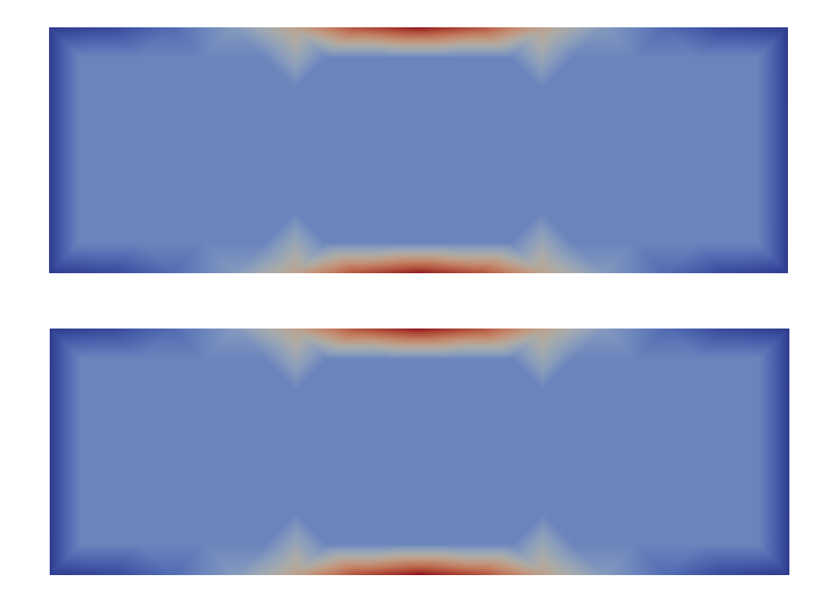
Dynamic state at (above) vs steady state (below)

While the turnpike property of the state and adjoints is verified numerically, the remaining assumptions can be checked analytically as follows. By the classical embeddings for any for , cf. [37, Sec. 7.1] or [1, Chap. V] and as the nonlinearity is cubic, the occurring superposition operators satisfy 2.7 for . Moreover, as compactly, the perturbation is -compact and generates an analytic semigroup on , and , cf. [8, Chap. III, Thm. 2.10]. Thus, assuming additionally a boundedness condition of the adjoint, Theorem 4.4 applies and we obtain the turnpike property for the adjoint in . Additionally by analyticity of the semigroup, the improved estimate of Theorem 5.1 holds and we get the estimate also in the space with and . In Figure 4 we observe the turnpike property for the adjoint in the -norm and also in the -norm.
8. Summary and outlook
This paper presented an interval turnpike result for the adjoints of finite- and infinite-dimensional nonlinear optimal control problems under the assumption of an interval turnpike on states and controls. We analyzed the case of stabilizable dynamics governed by a generator of a semigroup with finite dimensional unstable part satisfying a spectral decomposition condition. We have shown the desired turnpike property under continuity assumptions on the first-order optimality conditions. We illustrated our findings drawing upon a boundary controlled semilinear heat equation.
We briefly discuss possible directions of further research. A central assumption in the results of this work is the boundedness condition on the adjoint, i.e., . We have presented a very particular case in Example 6.3 where this bound holds, however, under the strict condition that the cost at the equilibrium has to vanish. It is desirable to prove the bound under milder conditions.
In Section 7 we verified the turnpike property of state and control only numerically. This is due to the fact that the verification of assumptions of global turnpike theorems via dissipativity, cf. Remark 6.2, is a highly non-trivial issue. In that context, suitable storage functions need to be constructed and we refer to [14] for a promising approach in that direction.
An inspection of the proofs of Sections 3 and 4 shows that, under suitable assumptions, it should be possible replace the control operator by an unbounded operator, which is, e.g., the case for boundary control. In that context, a concept like admissibility or assuming that solutions are classical solutions is a suitable replacement for boundedness of .
References
- [1] R. A. Adams. Sobolev Spaces. Academic Press, Amsterdam, Boston, 1975.
- [2] J. Appell and P. P. Zabrejko. Nonlinear Superposition Operators. Cambridge Tracts in Mathematics. Cambridge University Press, 1990.
- [3] A. Bensoussan, G. Da Prato, M. C. Delfour, and S. Mitter. Representation and control of infinite dimensional systems. Springer Science & Business Media, 2007.
- [4] T. Breiten and L. Pfeiffer. On the turnpike property and the receding-horizon method for linear-quadratic optimal control problems. SIAM Journal on Control and Optimization, 58(2):1077–1102, 2020.
- [5] E. Casas. Boundary control of semilinear elliptic equations with pointwise state constraints. SIAM Journal on Control and Optimization, 31(4):993–1006, 1993.
- [6] R. F. Curtain and H. Zwart. An introduction to infinite-dimensional linear systems theory, volume 21. Springer Science & Business Media, 1995.
- [7] T. Damm, L. Grüne, M. Stieler, and K. Worthmann. An exponential turnpike theorem for dissipative discrete time optimal control problems. SIAM Journal on Control and Optimization, 52(3):1935–1957, 2014.
- [8] K.-J. Engel and R. Nagel. One-Parameter Semigroups for Linear Evolution Equations. Springer-Verlag New York, 2000.
- [9] T. Faulwasser, M. Korda, C. N. Jones, and D. Bonvin. On turnpike and dissipativity properties of continuous-time optimal control problems. Automatica, 81:297–304, 2017.
- [10] T. Faulwasser and A. Murray. Turnpike properties in discrete-time mixed integer optimal control. IEEE Control Systems Letters, 4:704–709, 2020.
- [11] H. Goldberg, W. Kampowsky, and F. Tröltzsch. On Nemytskij operators in Lp-spaces of abstract functions. Mathematische Nachrichten, 155(1):127–140, 1992.
- [12] S. Götschel, A. Schiela, and M. Weiser. Kaskade 7 – A flexible finite element toolbox. Computers & Mathematics with Applications, 2020.
- [13] L. Grüne. Economic receding horizon control without terminal constraints. Automatica, 49(3):725–734, 2013.
- [14] L. Grüne and R. Guglielmi. On the relation between turnpike properties and dissipativity for continuous time linear quadratic optimal control problems. Math. Control Rel. Fields, 2020. To appear.
- [15] L. Grüne and M. A. Müller. On the relation between strict dissipativity and turnpike properties. Systems & Control Letters, 90:45–53, 2016.
- [16] L. Grüne, M. Schaller, and A. Schiela. Sensitivity analysis of optimal control for a class of parabolic PDEs motivated by model predictive control. SIAM Journal on Control and Optimization, 57(4):2753–2774, 2019.
- [17] L. Grüne, M. Schaller, and A. Schiela. Exponential sensitivity analysis for model predictive control of PDEs. urn:nbn:de:bvb:703-epub-4590-3, 2020.
- [18] L. Grüne, M. Schaller, and A. Schiela. Exponential sensitivity and turnpike analysis for linear quadratic optimal control of general evolution equations. Journal of Differential Equations, 268(12):7311–7341, 2020.
- [19] M. Gugat and F. Hante. On the turnpike phenomenon for optimal boundary control problems with hyperbolic systems. SIAM Journal on Control and Optimization, 57(1):264–289, 2019.
- [20] M. Gugat, E. Trélat, and E. Zuazua. Optimal Neumann control for the 1D wave equation: Finite horizon, infinite horizon, boundary tracking terms and the turnpike property. Systems & Control Letters, 90:61–70, 2016.
- [21] M. Hinze, R. Pinnau, M. Ulbrich, and S. Ulbrich. Optimization with PDE constraints, volume 23 of Mathematical Modelling: Theory and Applications. Springer, New York, 2009.
- [22] B. Jacob, C. Trunk, and M. Winklmeier. Analyticity and Riesz basis property of semigroups associated to damped vibrations. J. Evol. Equ., 8(2):263–281, 2008.
- [23] I. Lasiecka and R. Triggiani. Control Theory for Partial Differential Equations: Volume 1, Abstract Parabolic Systems: Continuous and approximation theories, volume 1. Cambridge University Press, 2000.
- [24] X. Li and J. Yong. Optimal Control Theory for Infinite Dimensional Systems. Birkhäuser, 1995.
- [25] J.-L. Lions. Optimal Control of Systems Governed by Partial Differential Equations. Springer-Verlag Berlin-Heidelberg, 1971.
- [26] J.-L. Lions. Exact controllability, stabilization and perturbations for distributed systems. SIAM review, 30(1):1–68, 1988.
- [27] J. v. Neumann. A model of general economic equilibrium. The Review of Economic Studies, 13(1):1–9, 1945.
- [28] A. Pazy. Semigroups of Linear Operators and Applications to Partial Differential Equations. Springer, New York, NY, 1983.
- [29] A. Porretta. On the turnpike property for mean field games. Minimax Theory and its Applications, 3(2):285–312, 2018.
- [30] A. Porretta and E. Zuazua. Long time versus steady state optimal control. SIAM Journal on Control and Optimization, 51(6):4242–4273, 2013.
- [31] J. P. Raymond and H. Zidani. Hamiltonian Pontryagin’s principles for control problems governed by semilinear parabolic equations. Applied Mathematics and Optimization, 39(2):143–177, 1999.
- [32] N. Sakamoto, D. Pighin, and E. Zuazua. The turnpike property in nonlinear optimal control — A geometric approach. In 2019 IEEE 58th Conference on Decision and Control (CDC), pages 2422–2427, 2019.
- [33] O. J. Staffans. Well-Posed Linear Systems. Cambridge University Press, 2005.
- [34] E. Trélat and C. Zhang. Integral and measure-turnpike properties for infinite-dimensional optimal control systems. Mathematics of Control, Signals, and Systems, 30(1):3, 2018.
- [35] E. Trélat, C. Zhang, and E. Zuazua. Steady-state and periodic exponential turnpike property for optimal control problems in Hilbert spaces. SIAM Journal on Control and Optimization, 56(2):1222–1252, 2018.
- [36] E. Trélat and E. Zuazua. The turnpike property in finite-dimensional nonlinear optimal control. Journal of Differential Equations, 258(1):81–114, 2015.
- [37] F. Tröltzsch. Optimal control of partial differential equations: theory, methods, and applications, volume 112. American Mathematical Soc., 2010.
- [38] A. J. Zaslavski. Turnpike theory of continuous-time linear optimal control problems. Springer, 2016.