Inverse-Chirp Imprint of Gravitational Wave Signals in Scalar Tensor Theory
Abstract
The scalar tensor theory contains a coupling function connecting the quantities in the Jordan and Einstein frames, which is constrained to guarantee a transformation rule between frames. We simulate the supernovae core collapse with different choices of coupling functions defined over the viable region of the parameter space and find that a generic inverse-chirp feature of the gravitational waves in the scalar tensor scenario.
I Introduction
The searches for gravitational waves (GWs) by the kilometric-size laser-interferometer systems, such as the Laser Interferometric Gravitational wave Observatory (LIGO) in US, Virgo in Italy and the KAmioka GRAvitational Wave Detector (KAGRA) in Japan, have been initiated to test various gravitational theories. Particularly, the gravity effects in the strong-field regime can be verified through the observations, where the underlying gravity theory may deviate from General Relativity (GR). In practice, several alternative theories of gravity have been proposed. Among them, the scalar tensor (ST) theory is the most natural extension to GR, in which gravity can be mediated by a scalar field in addition to the metric one. This additional field introduces the spontaneous scalarization phenomenon within the gravitation field of neutron stars Damour:1993hw, which is a non-perturbative deviation from GR. In a recent work Sperhake:2017itk, it has been shown that one can observe the presence of such phenomenon in the supernova core collapse scenario as well.
Furthermore, it has been proved by Damour and Esposito-Farèse Damour:1992we; Damour:1993hw that under the assumption that there exists a transformation between Jordan and Einstein frames, a two-parameter family of the ST theory is sufficient to parametrize the most general post-Newtonian deviations from GR with the nonperturbative strong-field effects. Many works have also been done along this direction Novak:1997hw; Novak:1998rk; Barausse:2012da; Berti:2013gfa; Llinares:2013qbh; Sperhake:2017itk. However, several problems related to the assumption have been discussed in the literature Faraoni:2004is; Flanagan:2004bz; Faraoni:2006fx; Brans:2005ra; Jarv:2015kga; Ishak:2018his; Geng:2020ftu. The transformation between two frames includes a Weyl transformation of metric and a redefinition of the scalar field, . It has been demonstrated in Jarv:2015kga; Geng:2020ftu that there is a criterion concerning the scalar field redefinition, which leaves a constraint on the parameter space of the coupling function defined in the Einstein frame Geng:2020ftu. In light of such criterion/constraint, it is prospective to further constrain the ST theory with the signals of GWs. To capture the features of those signals, we consider the stellar core collapse systems in the massive ST scenario.
In this work, we first express how the aforementioned criterion manifests itself as a constraint on the parameter space. We then numerically simulate the supernovae core collapse in the viable region of the parameter space by using the code in Sperhake:2017itk to study the profile of the genuine strong-field effects.
The paper is organized as follows. In Sec. II, we briefly introduce the theoretical framework of the ST theory by concentrating on the constraint on the scalar field. The numerical simulations of the supernovae core collapse are represented in Sec. III. Our conclusions are given in Sec. VI.
II Scalar Tensor Theory
The ST theory can be formulated in both Jordan and Einstein frames, which are conformally related. In the Jordan frame, the action takes the form
| (1) |
where and are the regular coupling functions of the scalar field , and corresponds to the action of ordinary matter. It has been revealed since the original Brans-Dicke paper appeared Brans:1961sx; Dicke:1961gz that another formulation of the theory is possible. Through a Weyl transformation
| (2) |
and a redefinition of the scalar field Geng:2020ftu
| (3) |
one can recast the theory into the so-called Einstein frame with the action, given by
| (4) |
where is the transformed metric, is the coupling function defined by , and . As a result, the field equations are the usual Einstein ones with the scalar field as a source together with an equation of motion of the scalar field, namely
| (5a) | ||||
| (5b) | ||||
where
| (6) |
and with the stress energy tensor
| (7) |
In the mathematical viewpoint, having the scalar field in the Einstein frame to be viable in the Jordan frame, one should be able to represent as a function of . Subsequently, the existence of indicates that Geng:2020ftu
| (8) |
Hence, the solution to the scalar equation in the Einstein frame must satisfy (8). Otherwise, it is not a solution to the scalar equation in the Jordan frame.
In this work, we adopt the conformal factor as discussed in Damour:1993hw; Damour:1996ke; Novak:1997hw; Novak:1998rk, given by
| (9) |
where is the asymptotic value of at spatial infinity. The constants and are defined as
| (10a) | ||||
| (10b) | ||||
The coupling function in (9) leads to
| (11) |
and
| (12) |
By substituting (11) into (5b), one obtains the equation of motion
| (13) |
where is the square of the effective mass for , defined by
| (14) |
In Damour:1993hw; Damour:1996ke, Damour and Esposito-Farése described the dramatic deviation from GR for some specific values of the coupling constants, dubbed as “spontaneous scalarization.” To trigger this sudden behavior of the scalar field, should be smaller than a specific value, which is for the static neutron stars, while it would increase a bit but still negative Doneva:2013qva for the rotating ones. In this study, we set that and .
The non-vanishing property of (8) together with the definition (6) implies that the parameter can never be zero, resulting in that there is a critical value for by (11), denoted as Geng:2020ftu, i.e.
| (15) |
This shows that the solution space of the scalar field in the Einstein frame is divided into two disconnected branches by the value of with to be a non-crossing line for the scalar field in the Einstein frame.
The metric in the Jordan frame is partially determined by , which is a field in the Einstein frame. Technically speaking, once one ensures that the signals from the simulation are reversible to the Jordan frame, the measurable amplitude of the scalar signal can be expressed as
| (16) |
where
| (17) |
and
| (18) |
which are the breathing and longitudinal modes of GWs, respectively Will:2014kxa. The amplitude of the longitudinal mode is proportional (up to a sign) to , and the coefficient depends on the Compton length of the scalar field, , hence to the effective mass term of . As a result, is clearly proportional to . We shall show that this amplitude has an inverse-chirp evolution along with , which is the key profile of the additional modes of GWs in the massive ST theory. Practically, the GW signals from the stellar collapse in the theory are monochromatic soon after the emission, which are likely detectable with the ground-based GW detectors Sperhake:2017itk.
III Numerical Simulations
We follow the method used in Sperhake:2017itk. The supernovae core collapse is considered with the spherically symmetric metric of the form
| (19) |
where all metric functions depend only on the coordinates and . We take matter as a perfect fluid, whose energy-momentum tensor in the Jordan frame can be expressed in the spherical coordinate as
| (20) |
where , and are the energy density, pressure and 4-velocity of matters, respectively. The enthalpy is defined by
| (21) |
where is the internal energy. The quantities are connected to those in the Einstein frame, labeled with the asterisk, via the relations
| (22a) | ||||
| (22b) | ||||
| (22c) | ||||
The field equations are solved numerically by utilizing the modification of the code introduced in Sperhake:2017itk, which is developed from GR1D OConnor:2009iuz. In the simulation, the hybrid equation of state (EOS) is used to account for the stiffening of the nuclear and model the response of the shocked material by the forms of and with the thermal effects, where the cold parts of pressure and internal energy are given as
| (23a) | ||||
| (23b) | ||||
where and [cgs] with and naturally followed by the continuity. An additional relation to close up Eqs. (22) and (23) is given by
| (24) |
Clearly, we have three parameters , set to be , to specify the EOS.
As a first study of the influence of the constraint in (8), we will present the results for a specific progenitor of the supernova core collapse, which is coded as WH20 in Gerosa:2016fri, along with the density of the atmosphere being 2 outside the progenitor. Note that our methodology can be generalized to all systems.
We consider the action
| (25) |
where the coupling function is given in (9). The effective mass can be obtained from (14)
| (26) |
If GWs are to be detectable inside the LIGO sensitivity window, the mass should be bounded above by eV since the low-frequency modes of GWs with will damp out instead of radiating outward to infinity Jackson:1998nia. In addition, the mass less than eV would not be able to generate the strong scalarization and satisfy binary pulsar constraints Gerosa:2016fri; Ramazanoglu:2016kul at the same time. Hence, we fix the mass to be eV hereafter.
In principle, one can define the coupling functions by fixing and in (11) with Sperhake:2017itk; Geng:2020ftu to carry out the simulation. To illustrate our results, we use the set containing pairs with a constant ratio of , namely
| (27) |
It is clear that is defined by a certain critical value. One can view the solutions of the scalar field for within as an one-parameter family curve by choosing as the parameter for the later analysis. In Fig. 1, we show that the amplitudes of the GW signals at the distance of cm away from the stellar core are too small by comparing with the critical value , where is a horizontal line far above the signals on the plot. One can further notice that the signals for the cases with and are obviously different from the others since they do not or barely possess the second twist before reaching the peak around . This will be explained next.

As introduced in roscamead2020core, the amplitudes of the signals at the wave zone of their propagations with different Compton lengths of the scalar field have an approximate universal relation. If we ignore the source term of in (13), the Compton length would be a function of , so that the signals within the same window have a homologous form. This universality is broken due to the presence of , which may be measured by the absolute value of the ratio between the coefficients of the zeroth and first order terms in on the right hand side of (13), given by
| (28) |
where . Consequently, we have that for as the linear term dominates, and otherwise. The behaviors of as a function of with several values of () are plotted on the left (right) panel of Fig. 2. For the signals in Fig. 1, our simulation on the right panel of Fig. 2 illustrates that there are deviations of from the first order dominating limitation when and , whereas they are about twice even three times as much as the cases with and . From Fig. 2, one can graphically see that the homologous form has been distorted for the later two cases.

For in Fig. 3, the amplitudes of the GW signals at the same extraction distance are comparable to those at the critical value , and hence the constraint is more stringent in this case. Any solution crossing the dashed line will be ruled out. In the cases shown in Fig. 3, is confined in with respective to , which is small enough so that the shapes of the signals do not deviate much.

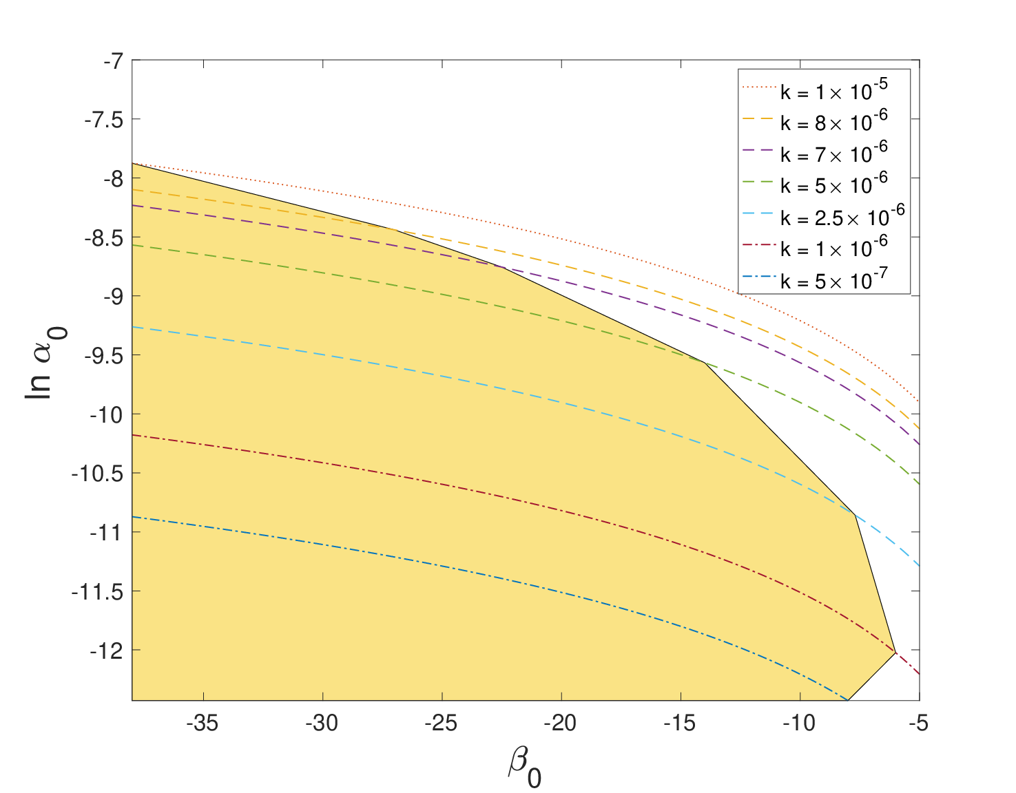
From Figs. 1 and 3, one can observe that as decreases, the peaks of the curves increase accordingly until they touch the non-crossing line. We can define the corresponding parameter as the critical value of , denoted by . As a result, there exists a value of such that the peak of reaches the value of . Consequently, any case with will be forbidden due to its crossing with the line of
In Fig. 4, we select seven values of , , , , , , and for as the constraints on . The parameter space is split into two pieces bounded by the solid curve, in which the parameters in the left (yellow) region are ruled out. This is to say, the Jordan and Einstein frames do not correspond to each other in the shade area in Fig. 4. We note that the shade area will change for the different initial data/progenitors as well as EOS.
We now discuss the dependence of our results on the hybrid EOS. The scalar field signal grows in the amplitude during the collapsing phase, while the central mass density increases. As the density gets beyond the nuclear density , the stellar core undergoes a short period of bounces. After this phase, the scalar field in the inner core tends to be a static profile, while the scalar radiation is generated outwards. During the process, and in Eqs. (23) and (24) related to the EOS only affect the wave signal during and after the bounces, so that the influence of the EOS on the scalar waves is mainly from . Explicitly, a larger would result in a more compact core at the moment of the bounce, while the stronger scalar waves would be released accordingly Gerosa:2016fri. This leads to a larger shaded area because the peak of the scalar field reaches the non-crossing line with a smaller . However, the inverse-chirp feature of the scalar radiations remains unchanged as long as one considers the viable parameter space.
Moreover, within the same parameter set of , the amplitude of the scalar field with a larger or is bigger. The contribution of the scalar field in the Einstein frame to the gravitational waveform in the Jordan frame comes through Eq. (5.6), given by Damour:1992we
| (29) |
which implies that the scalar field affects more as increases. However, to some extend, the solution will touch the non-crossing line and this puts the upper limit for the detectability of the contribution of the scalar field in GWs.
IV Conclusions
We have simulated the supernovae core collapse and found the generic feature of scalar GWs in the ST scenario with in the Einstein frame, which has an inverse-chirp behavior. We have shown that the ST theory should be defined in the viable region for the parameter space in order to have the signal to be recognized as GWs in the Jordan frame.
In particular, to ensure that one can transform the fields from the Jordan frame to Einstein one, and vice versa, there is a constraint on the parameter space in the ST theory. For the supernovae core collapse, we have illustrated the upper bound on for each in (27). Using the bounds for the different sets of , we have obtained the viable region for the parameters in the particular ST theory. In this area of the parameter space, we have carried out the numerical simulations with several pairs of .
Even though the intrinsic amplitude of the scalar field is insensitive to Sperhake:2017itk, the measurable scalar signal with the amplitude in terms of is closely related to the Weyl transformation associated with the viable region of these parameters. Furthermore, the constraint of the parameter would affect the contribution of the scalar mode in the gravitational waveform of the tensor mode, which has been shown in (29). Therefore, we have demonstrated that the inverse-chirp profile of the GW signals is generic so that it can be used as a probe to test the ST theory.
Acknowledgements.
We would like to thank Patrick Chi-Kit Cheong for useful discussions. The work was partially supported by National Center for Theoretical Sciences and Ministry of Science and Technology (MoST-107-2119-M-007-013-MY3 and MoST-108-2811-M-001-598).References
- (1) T. Damour and G. Esposito-Farèse, Phys. Rev. Lett. 70, 2220 (1993).
- (2) U. Sperhake, C. J. Moore, R. Rosca, M. Agathos, D. Gerosa and C. D. Ott, Phys. Rev. Lett. 119, 201103 (2017).
- (3) T. Damour and G. Esposito-Farèse, Class. Quant. Grav. 9, 2093 (1992).
- (4) J. Novak, Phys. Rev. D 57, 4789 (1998).
- (5) J. Novak, Phys. Rev. D 58, 064019 (1998).
- (6) E. Barausse, C. Palenzuela, M. Ponce and L. Lehner, Phys. Rev. D 87, 081506 (2013).
- (7) E. Berti, V. Cardoso, L. Gualtieri, M. Horbatsch and U. Sperhake, Phys. Rev. D 87, 124020 (2013).
- (8) C. Llinares and D. Mota, Phys. Rev. Lett. 110, 161101 (2013).
- (9) E. E. Flanagan, Class. Quant. Grav. 21, 3817 (2004)
- (10) V. Faraoni, Phys. Rev. D 70, 081501 (2004).
- (11) V. Faraoni and S. Nadeau, Phys. Rev. D 75, 023501 (2007)
- (12) C. H. Brans, gr-qc/0506063 (2005).
- (13) M. Ishak, Living Rev. Rel. 22, 1 (2019).
- (14) L. Järv, P. Kuusk, M. Saal and O. Vilson, Class. Quant. Grav. 32, 235013 (2015).
- (15) C. Q. Geng, H. J. Kuan and L. W. Luo, Class. Quant. Grav. 37, 115001 (2020).
- (16) C. Brans and R. H. Dicke, Phys. Rev. 124, 925 (1961).
- (17) R. H. Dicke, Phys. Rev. 125, 2163 (1962).
- (18) T. Damour and G. Esposito-Farese, Phys. Rev. D 54, 1474 (1996).
- (19) D. D. Doneva, S. S. Yazadjiev, N. Stergioulas and K. D. Kokkotas, Phys. Rev. D 88, 084060 (2013).
- (20) C. M. Will, Living Rev. Rel. 17, 4 (2014)
- (21) E. O’Connor and C. D. Ott, Class. Quant. Grav. 27, 114103 (2010).
- (22) J. D. Jackson, “Classical electrodynamics,” New York, NY: Wiley (1999).
- (23) D. Gerosa, U. Sperhake and C. D. Ott, Class. Quant. Grav. 33, 135002 (2016).
- (24) F. M. Ramazanoğlu and F. Pretorius, Phys. Rev. D 93, no. 6, 064005 (2016).
- (25) R. Rosca-Mead, U. Sperhake, C. J. Moore, M. Agathos, D. Gerosa and C. D. Ott, arXiv:2005.09728 (qr-qc).