Cosmic Inflation in Minimal Model: Implications for (Non) Thermal Dark Matter and Leptogenesis
Abstract
We study the possibility of realising cosmic inflation, dark matter (DM), baryon asymmetry of the universe (BAU) and light neutrino masses in non-supersymmetric minimal gauged extension of the standard model with three right handed neutrinos. The singlet scalar field responsible for spontaneous breaking of gauge symmetry also plays the role of inflaton by virtue of its non-minimal coupling to gravity. While the lightest right handed neutrino is the DM candidate, being stabilised by an additional symmetry, we show by performing a detailed renormalisation group evolution (RGE) improved study of inflationary dynamics that thermal DM is generally overproduced due to insufficient annihilations through gauge and scalar portals. This happens due to strict upper limits obtained on gauge and other dimensionless couplings responsible for DM annihilation while assuming the non-minimal coupling to gravity to be at most of order unity. The non-thermal DM scenario is viable, with or without symmetry, although in such a case the gauge sector remains decoupled from the inflationary dynamics due to tiny couplings. We also show that the reheat temperature predicted by the model prefers non-thermal leptogenesis with hierarchical right handed neutrinos while being consistent with other requirements.
I Introduction
Precision measurements of the cosmic microwave background (CMB) anisotropies by experiments like Planck Komatsu:2010fb; Akrami:2018odb; Aghanim:2018eyx reveal that our universe is homogeneous and isotropic on large scales upto a remarkable accuracy. However, the observed isotropy of the CMB leads to the horizon problem which remains unexplained in the standard cosmology where the universe remains radiation dominated throughout the early stages. In order to solve the horizon problem, the presence of a rapid accelerated expansion phase in the early universe, called inflation Guth:1980zm; Starobinsky:1980te; Linde:1981mu was proposed. Originally proposed to solve the horizon, flatness and unwanted relic problems in standard cosmology, the inflationary paradigm was also subsequently supported by the adiabatic and scale invariant perturbations observed in the CMB Komatsu:2010fb; Akrami:2018odb. Such an early accelerated phase of expansion can be generated by the presence of one or more scalar fields whose dynamics crucially decides the period of inflation. Over the years, a variety of inflationary models have been studied with different levels of success Mazumdar:2010sa. The earliest proposal of this sort is known as chaotic inflation Linde:1983gd; Martin:2013tda where simple power law potentials like with a scalar field were used. However, such simple models predict very specific values of inflationary parameters like the spectral index , tensor-to-scalar ratio for number of e-folds and unfortunately, the latest Planck 2018 data Akrami:2018odb strongly disfavour this simple model due to its large prediction of . Modified chaotic inflation where the inflation sector is extended by an additional scalar field to assist the inflaton field has also been proposed Harigaya:2015pea; Saha:2016ozn; Borah:2019bdi. Another class of models use the Higgs as the inflaton Bezrukov:2007ep; Bezrukov:2010jz. These models often suffer from problems of vacuum stability Sher:1988mj and non-unitarity Lerner:2009na as well as being inadequate for combining inflation with other cosmological problems like DM and BAU. A possible way out is to consider a beyond standard model (BSM) singlet scalar which acts as the inflaton. We consider this possibility in our work where an additional scalar with non-minimal coupling to gravity Pallis:2014cda; Gumjudpai:2016ioy; Tenkanen:2017jih; Shokri:2019rfi, in addition to usual quartic chaotic type coupling, can give rise to successful inflation while predicting the inflationary parameters within the observed range. The same scalar field is also responsible for several other interesting phenomenology as we discuss below.
The same CMB measurements mentioned above also suggest that the present universe has a significant amount of non-luminous, non-baryonic form of matter, known as dark matter (DM) Aghanim:2018eyx; Tanabashi:2018oca. This is also supported by astrophysical evidences gathered over a much longer period of time Zwicky:1933gu; Rubin:1970zza; Clowe:2006eq. The Planck 2018 data reveals that approximately of the present universe is composed of DM, which is about five times more than the ordinary luminous or baryonic matter. In terms of density parameter and , the present DM abundance is conventionally reported as Aghanim:2018eyx: at 68% CL. Since none of the standard model (SM) particles can satisfy the criteria of a particle DM candidate, several proposals have been put forward among which the weakly interacting massive particle (WIMP) is perhaps the most popular one. In this framework, a DM particle having mass and interactions typically around the electroweak scale can give rise to the observed DM abundance after thermal freeze-out, a remarkable coincidence often referred to as the WIMP Miracle Kolb:1990vq. The same interactions responsible for thermal freeze-out of WIMP type DM should also give rise to sizeable DM-nucleon scattering. However, null results at direct detection experiments like LUX Akerib:2016vxi, PandaX-II Tan:2016zwf; Cui:2017nnn, XENON1T Aprile:2017iyp; Aprile:2018dbl have certainly pushed several WIMP models into a tight corner, if not ruled out yet. This has also generated interests in beyond thermal WIMP paradigms as viable alternatives. One such interesting possibility is the non-thermal origin of DM Hall:2009bx. For a recent review of such feebly interacting (or freeze-in) massive particle (FIMP) DM, please see Bernal:2017kxu. In the FIMP scenario, DM candidate does not thermalise with the SM particles in the early universe due to its feeble interaction strength and the initial abundance of DM is assumed to be zero. At some later stage, DM can be produced non thermally from decay or annihilation of other particles thermally present in the universe.
Similarly, the baryonic content of the universe also gives rise to another puzzle due to the abundance of baryons over antibaryons. Quantitatively, this excess is denoted as baryon to entropy ratio Tanabashi:2018oca; Aghanim:2018eyx
| (1) |
where denotes comoving baryon density, denotes baryon (anti-baryon) number density while is the entropy density. Since any initial asymmetry before inflation will be washed out at the end of inflation due to the exponential expansion of the universe, there has to be a dynamical mechanism to generate the asymmetry in a post-inflationary universe. This requires certain conditions, known as the Sakharov conditions Sakharov:1967dj to be fulfilled. They are namely, baryon number (B) violation, C and CP violation and departure from thermal equilibrium, not all of which can be fulfilled in the required amounts within the SM alone. Generation of baryon asymmetry of the universe (BAU) from out-of-equilibrium decays of heavy particles has been a well-known mechanism for baryogenesis Weinberg:1979bt; Kolb:1979qa. Another interesting way, which also connects the lepton sector physics, is known as leptogenesis, proposed a few decades back Fukugita:1986hr. In leptogenesis, instead of creating a baryon asymmetry directly from B violating interactions, an asymmetry in lepton sector is created via lepton number (L) violating processes (decay or scattering). If this lepton asymmetry is generated before the electroweak phase transition (EWPT), then the -violating electroweak sphaleron transitions Kuzmin:1985mm can convert it to the required baryon asymmetry. Since the quark sector CP violation is insufficient to produce the required baryon asymmetry, the mechanism of leptogenesis can rely upon lepton sector CP violation which may be quite large as hinted by some neutrino oscillation experiments Esteban:2018azc; Abe:2019vii. An interesting feature of this scenario is that the required lepton asymmetry can be generated through CP violating out-of-equilibrium decays of the same heavy fields that take part in popular seesaw mechanisms Minkowski:1977sc; Mohapatra:1979ia; Yanagida:1979as; GellMann:1980vs; Glashow:1979nm; Schechter:1980gr which also explains the origin of tiny neutrino masses Tanabashi:2018oca, another observed phenomena which the SM fails to address.
Motivated by these, we study a minimal extension of the SM, by a gauged symmetry with three right handed neutrinos (RHN) required to cancel the anomalies and a singlet scalar to break the additional gauge symmetry spontaneously while simultaneously generating RHN masses. Although previously analysed separately, the consistency of these three entities together have not been examined in this simple kind of BSM setup before as per our knowledge. We also perform a complete RG evolution of all the relevant couplings to determine the fate of the scenarios we discuss here. While in this framework, the singlet scalar plays the role of inflaton, one RHN is stabilised by an additional symmetry to become a DM candidate. The other two RHNs can give rise to light neutrino masses with vanishing lightest neutrino mass apart from producing the required lepton asymmetry which gets converted into the observed baryon asymmetry via sphalerons. Interestingly, we find that the stringent limits on the inflationary observables from Planck 2018 and BICEP 2 / Keck Array (BK15) data Akrami:2018odb as well as the stability of inflaton potential restrict the gauge coupling, scalar couplings and Yukawa couplings associated with the inflaton field to be within some limits which do not favour thermal DM scenario due to insufficient annihilations. As an alternative, with very tiny gauge and Yukawa couplings, one can realise the non-thermal DM scenario (with or without symmetry) while the inflationary potential behaviour merges with the usual case of quartic inflation with non minimal coupling to gravity. We also find that the predicted values of reheat temperature makes it difficult to realise high scale thermal leptogenesis DiBari:2005st; Mahanta:2019gfe with hierarchical RHN leaving the option of non-thermal leptogenesis Lazarides:1991wu; Giudice:1999fb; Asaka:1999yd; Asaka:1999jb; Fujii:2002jw; Pascoli:2003rq; Asaka:2002zu; Panotopoulos:2006wj; HahnWoernle:2008pq viable.
The structure of the paper is organised as follows. In section II, we discuss the particle content of the proposed setup and their interactions followed by brief mention of the existing constraints in section III. In section IV we perform a detailed study of inflation and its predictions in view of Planck 2018 bounds. We discuss different aspects of DM phenomenology in section V and then move onto discussing the possibility of non-thermal leptogenesis in section VI. Finally we conclude in section VII.
II The Model
As mentioned earlier, we study a gauged extension of the SM with the minimal field content which can give rise to cancellation of triangle anomalies, spontaneous gauge symmetry breaking, light neutrino masses, dark matter, leptogenesis and cosmic inflation. While gauged extension of the SM was proposed long ago Davidson:1978pm; Mohapatra:1980qe; Marshak:1979fm; Masiero:1982fi; Mohapatra:1982xz; Buchmuller:1991ce, realising a stable DM candidate in the model requires non-minimal field content or additional discrete symmetries. Also, a gauged model with just SM fermion content, is not anomaly free due to the non-vanishing triangle anomalies for both and mixed anomalies. These triangle anomalies for the SM fermion content are given as
| (2) |
Remarkably, if three right handed neutrinos with charge -1 each are added to the model, they contribute leading to vanishing amount of triangle anomalies. This is perhaps the most economical setup of anomaly cancellation and hence we adopt it here 22 2 For other exotic solutions to anomaly cancellation conditions, see Montero:2007cd; Wang:2015saa; Patra:2016ofq; Nanda:2017bmi; Bernal:2018aon; Biswas:2019ygr; Nanda:2019nqy.. To have a stable DM candidate we introduce a discrete symmetry under which one of the RHN is odd whereas all other fields are even. In Tables 1 and 2, we have listed all fermions as well as scalar fields (including the SM ones) of the present model and their charges under the symmetry.
| Particles | ||
|---|---|---|
| + | ||
| + | ||
| + | ||
| + | ||
| + | ||
| - | ||
| + | ||
| + |
| Particles | ||
|---|---|---|
| + | ||
| + |
The gauge invariant Lagrangian of the model is
| (3) |
where denotes the SM Lagrangian involving quarks, gluons, charged leptons, left handed neutrinos and electroweak gauge bosons while the second term is the kinetic term of gauge boson () expressed in terms of field strength tensor . The gauge invariant scalar Lagrangian of the model is as follows
| (4) |
where
| (5) |
The covariant derivatives of scalar fields are
| (6) | ||||
| (7) |
with and being the gauge couplings of and respectively and () and are the corresponding gauge fields. On the other hand are the gauge boson and gauge coupling respectively for gauge group.
The gauge invariant fermionic Lagrangian of the model is as follows
| (8) |
The covariant derivative is defined as
| (9) |
with being the charge of right handed neutrino . Due to the presence of symmetry, has no mixing with and also does not interact with SM leptons thereby qualifying for a stable DM candidate.
After breaking of both symmetry and electroweak symmetry by the vacuum expectation values (VEVs) of and , the form of doublet and singlet scalar fields are given by,
| (10) |
where and are VEVs of and respectively. The right handed neutrinos and get masses after the breaking as,
| (11) | ||||
| (12) |
Here we consider diagonal Yukawa in basis. Using equation (11) and equation (12), it is possible to relate and by,
| (13) |
Also after the breaking of , the scalar fields and can be related to the physical mass eigenstates and by a rotation matrix as,
| (14) |
where the scalar mixing angle is represented by
| (15) |
The physical scalar masses are given by,
| (16) | ||||
| (17) |
Here is identified as the SM Higgs mass whereas is the singlet scalar mass.
One of the strong motivations of the minimal model is the presence of heavy RHNs which can yield correct light neutrino mass via type I seesaw mechanism. The analytical expression for the light neutrino mass matrix is
| (18) |
where . We consider the right handed neutrino mass matrix to be diagonal. Since in our case does not interact with SM leptons, the lightest active neutrino would be massless. The Dirac neutrino Yukawa matrix can be formulated through the Casas-Ibarra parametrisation Casas:2001sr as
| (19) |
where are the diagonal light and heavy neutrino mass matrices respectively and is the usual Pontecorvo-Maki-Nakagawa-Sakata (PMNS) leptonic mixing matrix. In the diagonal charged lepton basis, the PMNS mixing matrix is also the diagonalising matrix of light neutrino mass matrix
In the above Casas-Ibarra parametrisation, represents a complex orthogonal matrix (). In case of only two right handed neutrinos, the matrix is a function of only one complex rotation parameter Ibarra:2003up. For three right handed neutrinos taking part in seesaw mechanism can depend upon three complex rotation parameters. Assuming one of them (rotation in 1-2 sector) to be vanishing, it can be represented as33 3 For some recent discussions on choice of matrix in the context of thermal and non-thermal dark matter as well as leptogenesis, please see Mahanta:2019gfe.
| (20) |
Therefore with suitable choices of and , the Yukawa matrix can take different forms. Here it remains pertinent to note that for a symmetric Lagrangian () as described in equation (8), the Dirac Yukawa coupling represents a matrix in flavour basis. We shall use the best fit values of all three mixing angles and the mass squared differences of active neutrinos assuming a normal ordering Tanabashi:2018oca.
III Constraint on the Model Parameters
In this section, we briefly discuss the theoretical and experimental constraints on different parameters of the model.
To begin with, we consider the bounded from below criteria of the scalar potential. This gives rise to the following conditions to be satisfied by the quartic couplings,
. On the other hand, to avoid perturbative breakdown of the model, all dimensionless couplings must obey the following limits at any energy scale:
The non-observation of the extra neutral gauge boson in the LEP experiment Carena:2004xs; Cacciapaglia:2006pk invokes following constraint on the ratio of and :
| (21) |
The corresponding bounds from the large hadron collider (LHC) experiment have become stronger than this by now as both the ATLAS and the CMS collaborations have performed dedicated searches for dilepton resonances in proton-proton collisions. The latest bounds from the ATLAS experiment Aaboud:2017buh; Aad:2019fac and the CMS experiment Sirunyan:2018exx at the LHC rule out such gauge boson masses below 4-5 TeV from analysis of 13 TeV centre of mass energy data. However, such limits are derived by considering the corresponding gauge coupling to be similar to the ones in electroweak theory and hence the bounds become less stringent for weaker gauge couplings Aaboud:2017buh. Additionally, if such Abelian gauge bosons couple only to the third generation leptons, then the collider bounds get even weaker, as explored recently in a singlet-doublet fermion DM scenario by the authors of Barman:2019aku.
Additionally, the singlet scalar of the model is also constrained Robens:2015gla; Chalons:2016jeu as it can mix with the SM Higgs and hence can couple to SM fields. The strongest bound on such mixing in scalar singlet extension of the SM arises from boson mass correction Lopez-Val:2014jva at NLO. For singlet scalar mass GeV, the singlet-SM Higgs mixing is constrained to be . For heavier singlet scalar masses GeV, the bounds from the requirement of perturbativity and unitarity of the theory turn dominant which gives . On the other hand, for lighter singlet scalar masses GeV, the LHC and LEP direct search Khachatryan:2015cwa; Strassler:2006ri and Higgs signal strength measurement Strassler:2006ri constrain the mixing angle as . If the singlet scalar is even lighter say, lighter than SM Higgs mass , SM Higgs can decay into a pair of singlet scalars. Latest measurements by the ATLAS collaboration restrict such SM Higgs decay branching ratio into invisible particles to be below ATLAS:2020cjb at CL.
IV Inflation
In this section, we describe the dynamics of inflation in detail and its predictions in view of the present experimental bounds. We identify the real part of singlet scalar field as the inflaton. Along with the renormalisable potential in equation (5), we also assume that is non-minimally coupled to gravity. For earlier studies in this context, please see Okada:2011en; Okada:2015lia and references therein. Related studies in supersymmetric gauged model can be found in Buchmuller:2012wn. For works guided by the same unifying principle of inflation, dark matter and neutrino mass, one may look at Allahverdi:2007wt; Kazanas:2004kv; Dong:2018aak; Borah:2018rca as well as references therein.
We denote the inflaton field as hereafter, which is same as the notation used for real part of field in earlier sections. Thus the potential responsible for inflation is given by
| (22) |
where stands for the Ricci scalar and is a dimensionless coupling of singlet scalar to gravity. We have neglected the contribution of in equation (22) by considering it to be much lower than the reduced Planck mass . The action for in Jordan frame takes the following form (apart from the couplings to the fermions and SM Higgs)
| (23) |
where , is the spacetime metric in the convention, stands for the covariant derivative of containing couplings with the gauge bosons which just reduces to the normal derivative (since during inflation, there are no fields other than the inflaton).
In order to simplify the calculations, we make the following conformal transformation to write the action in the Einstein frame Capozziello:1996xg; Kaiser:2010ps:
| (24) |
so that it looks like a regular field theory action with no explicit couplings to gravity. In the above transformation, represents the metric in the Einstein frame. To make the kinetic term of the inflaton canonical, we redefine by
| (25) |
where is the canonical field. Using these inputs, the inflationary potential in the Einstein frame can be written as,
| (26) |
where is identical to in equation (22). We then make another redefinition: and reach at a much simpler from of given by
| (27) |
Note that for an accurate analysis, one should work with renormalisation group (RG) improved potential and in that case, in equation (27) will be function of such that,
| (28) |
The one loop renormalisation group evolution (RGE) equations of the relevant parameters associated with the inflationary dynamics are given by,
| (29) | ||||
| (30) | ||||
| (31) | ||||
| (32) |
where we define , , and and . The RGE equations for rest of the couplings are provided in Appendix A.
We choose the heavy neutrino mass spectrum, satisfying the hierarchy and a diagonal RH neutrino mass matrix. Note that, from this section onwards, we are denoting the RHNs as only without denoting the chirality explicitly. For simplicity, we denote . Thus the right handed neutrino mass hierarchy implies . Let us first analyse the case where the RG running of is dominated by and . Then equation (29) can be rewritten as,
| (33) |
We ignore the contributions of and in the R.H.S. of equation (33) considering them to be negligible44 4 Unless the non-minimal coupling is very large, the self-quartic coupling of inflaton must be very small in order to be in agreement with correct inflationary parameters Okada:2010jf.. Since is very small, or can cause sharp changes in value from its initial magnitude during the evolution. It may also happen that becomes negative at some energy scale. Then the inflationary potential would turn unstable along field direction. Therefore the most acceptable case is to make at least during inflation so that the inflationary potential remains stable Okada:2015lia. To ensure , the equality has to be maintained, where we have assumed . We can further simplify the expression for by assuming . In Fig. 1, we show the RG running of as a function of for different values of considering (left panel) and (right panel) . The running for is shown in blue colour while the other colours represent the cases where the condition gets violated by . Fig. 1 clearly points out that indeed a small violation of the criteria can cause sharp instability of the inflationary potential.


In upper left panel of Fig. 2, we show the behaviour of the inflationary potential as a function of for different values of considering . The value of is determined from the equality earlier defined. As it can be observed, with the increase of , the potential starts to develop a local minimum


near some value say, . If such a local minimum exists, then the field could be trapped there and the inflaton will stop rolling. This provides an upper bound on such that the local minimum of does not appear. The existence of a local minimum can be further confirmed if near . This condition can be rewritten as
| (34) |
We plot in upper right panel of Fig. 2 as a function of . We observe that for , the inflationary potential indeed develops a local minimum near . Similar conclusion can be drawn for as shown in lower panel of Fig. 2 . One important point to be noted is that the value of gets enhanced with the increase of . We illustrate this in Fig. 3 where is plotted against different values of .

Next, we move on to calculate the predictions for inflationary observables. In terms of the original field , the slow roll parameters () and number of e-folds () are found to be
| (35) | ||||
| (36) | ||||
| (37) |
respectively. The inflationary observables such as spectral index (), tensor to scalar ratio () and scalar perturbation spectrum () can be expressed in terms of the slow roll parameters as
| (38) |
All these quantities have to be determined at the horizon exit of the inflaton () and we consider the number of e-folds for the numerical analysis. We perform a numerical scan over and to estimate the inflationary observables and considering . The initial value of is determined to produce the correct observed value of scalar perturbation spectrum at horizon exit. In Fig. 4 we show the variation of with to be consistent with the observed value of .

It turns out that the value of does not change much with the variation of for a constant value of since at inflationary energy scale. Contrary to this, value of is quite sensitive to . We see from left panel of Fig. 5 that increases with the enhancement of for different values of . The rate of increase of with turns flatter with the rise of value. In the right panel of Fig. 5 we plot contours for different values and by varying in the range 0.001-1. For comparison purpose we also insert the Planck 2018+BAO+BK15 1 and bounds Akrami:2018odb. It is evident that the present setup is able to provide set of values, consistent with the experimental constraints. Finally, in the left panel Fig. 6, we constrain the plane which correctly produces the values consistent with Planck (red) and (brown) bounds.


So far we have discussed the case where at inflationary energy scale. Hence, it is obvious to consider the opposite limit of these parameters. When , automatically the inflation scenario merges with the case of quartic inflation and non minimal coupling of inflaton to gravity as originally studied in Okada:2010jf. For completeness purpose we discuss this particular case in right panel of Fig. 6 in plane. As it is seen the contour can still satisfy the Planck 2018 bounds for . The contour of observed value of in plane remains same as in Fig. 4.
IV.1 Reheating
Once inflation ends, the thermalisation of the universe, leading to a radiation dominated universe has to be ensured. This is the reheating epoch Allahverdi:2010xz, which takes the universe from the inflationary phase to the radiation-dominated phase.
Originally, the reheating process was proposed as the perturbative decay of inflaton field into lighter degrees of freedoms Albrecht:1982. During oscillation, the energy of inflaton gets transferred into the relativistic lighter decay products. Approximately, the amount of energy density of the radiation bath is obtained as where is the total decay width of inflaton. Considering inflaton decay into radiation only while setting up thermodynamic equilibrium quickly after the decay, the maximum reheating temperature of the universe is found to be
| (39) |
where is the number of relativistic degrees of freedom in the thermal bath.
However, the success of this perturbative decay mechanism of inflaton is somewhat limited. In initial stages of reheating, the phenomena of parametric resonance might be important and may lead to explosive particle production which the theory of perturbative reheating does not take into account. This dynamics is known as preheating Kofman:1994; Kofman:1997; Greene:1997. In particular, if the oscillation amplitude of the inflaton is sufficiently large, the number density of the produced bosonic particles might be enhanced () due to the effects related to Bose statistics. In an expanding universe, this process occurs in a stochastic manner, and is known as stochastic resonance. The produced particles, due to the large amplitude of inflaton, turn non-relativistic and further decay into lighter relativistic particles. The primary condition which needs to be satisfied to attain parametric resonance in an inflationary framework is that the decay width of non-relativistic particles should be less than its production rate. Parametric resonance halts once the inflation oscillation amplitude becomes small and the resonance becomes narrower.
The presence of parametric resonance as described above could raise the final reheating temperature compared to the one obtained by considering the perturbative reheating only. However, if the couplings of the inflaton with the lighter particles are not strong enough, the resonance is narrow or not broad enough. This makes preheating inefficient. In particular, it was shown in ref. Kofman:1997; Greene:1997 that for couplings the broad resonance does not take place (resulting Kofman:1997; Felder:1999) and preheating finishes at very early stage without posing significant impact on the final reheating temperature. In that case the reheating temperature of the universe is dominantly guided by the perturbative reheating.
From the inflationary perspective, we are having two different kind of scenarios having phenomenological relevance namely, (i) and (ii) .
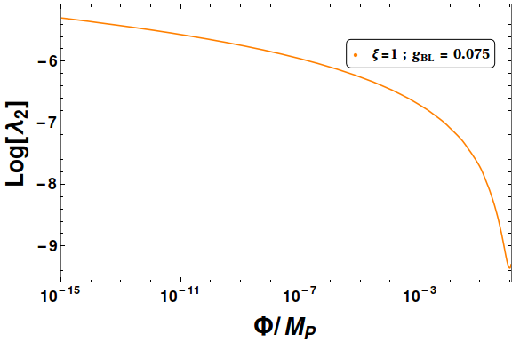

For the first case is large and thus is an essential condition for the stability of inflationary potential. We consider so that it does not effect the evolution of significantly. This assumption was made earlier also while determining the fate of inflation. The value of as defined earlier changes by small amount in its RG evolution (see right panel of Fig. 7). It is found that the value of changes by order of magnitudes at low scale, for example becomes from at inflationary scale (considering , see left panel of Fig. 7). During preheating stage, first , SM bosons get produced during the oscillation regime. Afterwards due to inflaton induced large mass these produced and SM bosons turn non-relativistic, and they decay into the lighter relativistic particles. In a whole, this particular process comprises of unusual stochastic resonance production of lighter non relativistic particles, their further decays, backreaction in the presence of an expanding universe. Hence the estimate of the correct reheating temperature is more involved and requires rigorous lattice simulation Garcia:2009; Maity:2019. Since we shall see in a while that this scenario turns out to be disfavoured due to overproduction of WIMP DM relic, we do not elaborate on this further55 5 In refs. Bezrukov:2009; Borah:2018rca a detailed analysis on preheating in a similar setup has been performed considering ..

‘
In the second case , the inflationary potential is mainly driven by with other couplings sufficiently small. Hence is not a necessary condition for this case. However the coupling (we take ) should be still much smaller than unity so that the stability of inflation potential remains intact. Here, due to the smallness of all relevant couplings there will not be any significant changes during their RG running unlike in the earlier case. The important point is with the estimates of and from inflation, the preheating stage never turns efficient and gets over at very early stage of inflaton oscillation. Then the reheating of the universe will be effectively dictated by the perturbative decay of inflaton. Here, depending on the mass scale (or ), the tree level decay of inflaton into final states are possible. The inflaton can also decay into right handed neutrinos, if kinematically allowed. In Fig. 8 we show the contours of different values of (ranging from GeV) in plane. For this purpose we fix GeV, TeV and TeV. The orange coloured region is ruled out from the requirement of reproducing the observed value of scalar perturbation spectrum at horizon exit. In the blue coloured region inflaton mass turns larger than the reheating temperature and hence it remains out of equilibrium. This may have important implications for other related phenomenology as we will discuss in a while.
V Dark matter
In this section, we discuss the dark matter phenomenology in detail and attempt to find its consistency with the inflationary dynamics. As mentioned earlier, is the DM candidate which is odd under and hence stable. For earlier studies of DM in this model, one may refer to Okada:2010wd; Basak:2013cga; Okada:2016gsh; Okada:2018ktp; Escudero:2018fwn. While the odd RHN is the DM candidate, the other two RHN’s take part in the usual type I seesaw mechanism, giving rise to light neutrino masses and mixing. Since DM is a singlet under SM gauge symmetry, it can interact with the visible sector particles only via gauge or scalar interactions. Now, depending upon the two cases namely, (i) and (ii) discussed in the context of inflation, DM-SM couplings can either be of order unity or very small. This will lead to completely different DM phenomenology namely, thermal or WIMP type and non-thermal or FIMP type, which we discuss separately below.
For the first case, that is, , it is expected that the DM stays in thermal equilibrium with the SM particles in the early universe and thus falls into the WIMP category. The DM can annihilate into different final states in the thermal bath through processes mediated by scalars and the gauge boson. In Fig. 9, we exhibit the possible annihilation processes of in the present framework. Please note that, in principle, the symmetry of the model allows a kinetic mixing term between of SM and of the form where and is the mixing parameter. Even if we turn off such mixing at tree level as we have done here, one can generate such mixing at one loop level since there are particles in the model which are charged under both and . Such one loop mixing can be approximated as Mambrini:2011dw. Since has tight upper bound from inflationary dynamics, the one loop mixing can be neglected in comparison to other relevant couplings and processes. Therefore, for simplicity, we ignore such kinetic mixing for the rest of our analysis.
V.1 WIMP DM Scenario


The evolution of comoving number density of DM () is determined by the corresponding Boltzmann equation
| (40) |
where
| (41) |
with and being the internal degrees of freedom of the dark matter and relativistic entropy degrees of freedom respectively and . The in equation (40) stands for the thermally averaged cross section of DM annihilation, given by Gondolo:1990dk
| (42) |
where ’s are modified Bessel functions of order . represents the Hubble parameter at .
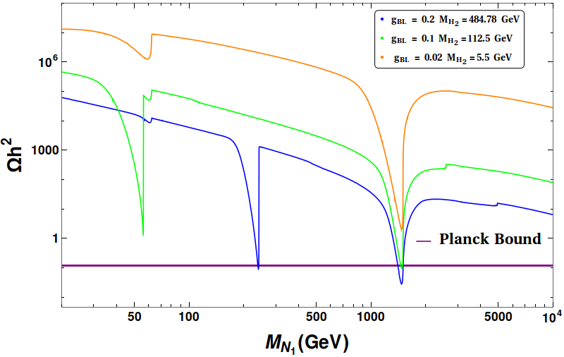

We implement the model in FeynRules Alloul:2013bka and then use micrOMEGAs package Belanger:2013oya to estimate the relic abundance of DM numerically. The independent parameters which participate in determining the DM relic abundance are the following:
| (43) |
In our case, we have considered the matrix diagonal and the sum of fourth power of each diagonal elements are fixed by inflationary requirements. However, for the DM analysis we need the magnitude of each individual elements. For simplification purpose we make the choice at the inflationary energy scale, to reduce the number of free parameters. The condition was essential at the inflationary energy scale and hence for the DM analysis we need to run the RGE equations of and along with and , with the initial condition , to estimate their values around few TeV scale, relevant for DM freeze-out. The value of will be fixed from the choice of DM mass and then the magnitude of ’s can be computed using values obtained at TeV scale through RG running. Since is taken to be smaller than , DM mass is smaller than ’s. We have already discussed the Dirac neutrino Yukawa or matrix and here we use the same form as defined in equation (19) using Casas-Ibarra parametrisation. Here we work with (corresponding to , see Fig. 4), at inflationary energy scale. Since in our working range of gauge coupling , the reheating temperature is expected to be large, hence it is obvious that the relevant SM and BSM fields will maintain thermal equilibrium with each other.
In Fig. 10, we show the variation of relic as function of DM mass for different set of values (at inflationary energy scale) by keeping fixed at 3 TeV. The order of magnitude of and are determined at TeV scale through their RG running corresponding to different mass and mixing. With the choices of different mass scales, three resonances appear for lines at and respectively. In some cases, one of the scalar resonances is not so prominent due to smallness of mass or mixing. The purple solid line in Fig. 10 represents the observed relic abundance, as per Planck 2018 data Aghanim:2018eyx. It is seen that the annihilation through gauge boson is the most efficient one and can satisfy correct relic in two out of three scenarios discussed.

We then perform a numerical scan to find the parameter space satisfying correct DM relic. In Fig. 11, we display the points satisfying correct DM relic (black dots) in plane considering TeV. We use the values of relevant parameters as earlier mentioned. We also include the LHC bound from dilepton resonance searches Aaboud:2017buh (red curve), Planck constraints on inflation and stability bounds of the inflationary potential for comparison purpose. The shaded regions are disfavoured from the respective constraints. To conclude, we observe that with TeV scale or lower mass, it is not possible to generate the correct value of relic abundance for WIMP dark matter while being in agreement with LHC and inflationary observables simultaneously. We also check that direct detection limits on spin-independent DM-nucleon cross section from the XENON1T experiment Aprile:2017iyp; Aprile:2018dbl and find that such bounds do not put any additional constraint on this parameter space as all the points shown in Fig. 12 obey these bounds.
V.2 FIMP DM Scenario
In the second case (), the couplings responsible for DM-SM interactions are tiny and hence it is expected that DM may never reach thermal equilibrium with the standard bath. This falls under the ballpark of FIMP dark matter, discussed earlier. For earlier work on fermion singlet as FIMP DM in model, please see Biswas:2016bfo; Biswas:2016iyh and references therein. A recent study also discussed the possibility of scalar singlet responsible for breaking gauge symmetry spontaneously to be a long-lived FIMP DM candidate Mohapatra:2020bze. If is a FIMP candidate, it can be produced non-thermally, due to decay or annihilation of other particles. In case symmetry is exact, will be only pair produced as it is the only odd particle. All scattering processes shown in Fig. 9 while discussing WIMP scenario can potentially contribute to the production of FIMP DM as well, when considered in the reverse direction. In addition, decays of and , if kinematically allowed, can also contribute to the relic density of . Typically, if same dimensionless couplings govern the strength of both decay and annihilation processes, the former dominates simply due to power counting. This is precisely the scenario here and FIMP is primarily produced from decays.
For our numerical calculation, we choose at inflationary energy scale corresponding to from inflationary requirements (see Fig. 4). Then from Fig. 8, it is evident that for this choice of , would be in thermal equilibrium with other SM particles by virtue of its coupling with Higgs as well as heavy right handed neutrinos which also maintain equilibrium since their masses considered here are below and they can interact to SM fields through Yukawa interaction. We would like to keep extremely small so that it does not alter the RG running of during inflation. Since is also very small to justify FIMP nature of DM, we will investigate the possibility of production of DM from non thermal tree level decays of and (see Fig. 13). We will consider two benchmark choices of TeV for the analysis. It is to be noted that which interacts only via gauge coupling is also expected to be out of equilibrium. Hence non-thermal production of from other bath particles and its subsequent decay into pairs play non-trivial roles. We therefore use coupled Boltzmann equations for both and to calculate the relic abundance of in this scenario.
The evolution of the comoving number densities for and DM are governed by the following coupled Boltzmann equations Biswas:2016bfo
| (44) | ||||
| (45) |
where and represents all possible initial states. is defined by
| (46) |
while is same as defined earlier. Here, denotes the effective number of degrees of freedom related to the energy density of the universe at . The denotes the thermally averaged decay width which is given by
| (47) |


Since initial densities of both and are almost vanishing, one can ignore and from first term within each bracket on right hand side of equations (44) and (45).
In left panel of Fig. 14, we show the evolution of against for benchmark choices of and other relevant parameters indicated in the figure. It is seen that starts from a vanishingly small value initially and reaches a sizeable value with the lowering of temperature very quickly. The initial increase in abundance happens primarily from decays. As expected, the production of from decay becomes efficient around which corresponds to . For there is a Boltzmann suppression in the equilibrium abundance of which makes production less efficient leading to the plateau region where remains more or less constant. We also observe that a larger value of while keeping fixed gives larger yield for . The reason behind this is two-fold. Firstly, the partial decay width of into pairs rises with the increase in values for our chosen benchmark points. Note that this partial decay width is function of and can be expressed as (in the limit )
| (48) |
Now, increase in corresponds to smaller as evident by combining equations (17) and (11) for a fixed . Hence in general, enhancement of does not always mean higher value of . However numerically, we find that for the chosen benchmarks of Fig. 14, even though decreases with increase in , the above decay width still increases by a factor of order one which enhances the yield of by some amount. Secondly, a lighter will have comparatively lesser Boltzmann suppression in its equilibrium number density. These two factors, with the latter being dominant, lead to the enhancement of (approximately by order of two), given other relevant parameters remain same. The production of from decay will be mixing suppressed due to smallness of . It is in fact kinematically forbidden for the chosen benchmark values of mass. For some epochs the abundance of remains constant (denoted by the plateau region) and then gets reduced to zero again due to subsequent decays of into as well as other lighter particles.

Similar features can be observed in right panel of Fig. 14 where the evolution of abundance is shown using the same choice of parameters as in left panel. The abundance begins from vanishingly small value and gets enhanced due to non-thermal production from and decays and finally gets saturated. We notice that larger value leads to larger final abundance of the DM due to both the enhanced abundance of (as earlier mentioned) as well as larger partial decay width of into DM pairs. It is also relevant to mention here that in our working regime , the associated Yukawa coupling () with is suppressed compared to and hence direct production of DM is primarily dominated from tree level decay.
Once the freeze-in abundance of DM that is saturates, one can obtain the present relic abundance using the following expression:
| (49) |
Here , where is the DM energy density and is the critical energy density of the universe, with being Newton’s gravitational constant and is the present-day Hubble expansion rate.
Using the above equation (49), we now find some benchmark parameters of our model which satisfy the correct DM abundance in the present universe. In Fig. 15, we have shown the DM yield evolutions for two set of parameters that matches with the observed relic bound (green shaded region) at . In table 3 we list the numerical values of the parameters used in Fig. 15. As mentioned earlier, for such benchmark values of parameters the contribution of scattering processes to DM production in the present analysis remains sub-dominant or negligible. It should be noted that while the required FIMP DM relic abundance can be successfully generated in this model, the corresponding parameter space leads to decoupling of gauge sector from inflationary dynamics leading to a usual quartic plus non-minimal inflation Okada:2010jf.
| GeV | GeV | |||||
| 100 GeV | GeV |
So far, the analysis on non thermal production of dark matter is performed by assuming in thermal equilibrium with the SM bath. This is possible when and has sizeable couplings with other particles in the bath. However, it is also possible that remains larger compared to the reheat temperature and hence the inflaton remains out of equilibrium afterwards (see blue coloured region of Fig. 8). In such a case, the production of and will not be possible like the way it was discussed before. Since SM Higgs mixing with is also very small, it is not possible to generate correct FIMP abundance. While interactions by virtue of gauge coupling and Yukawa coupling with are insufficient to produce correct FIMP abundance, one can turn to Yukawa couplings with ordinary leptons which are present in thermal bath for most of the epochs. However one has to get rid of the symmetry in order to introduce such Yukawa couplings through SM Higgs. We briefly discuss this possibility in the remainder of this section.
Once the symmetry is discarded, one can have new non-diagonal terms in the RHN mass matrix. However, for simplicity we continue to choose a diagonal RHN mass matrix or the corresponding Yukawa coupling matrix . The newly introduced Yukawa couplings of to SM leptons can be written as
| (50) |
This will generate mixing of with active neutrinos once the electroweak symmetry is broken. Using Casas-Ibarra parametrisation of equation (19) and using the form of complex orthogonal matrix given in equation (20), the Yukawa coupling of with leptons can be expressed as
| (51) |
where is a complex angle and the heaviest active neutrino mass with normal ordering. In deriving this, we fix Dirac CP phase to be zero66 6 Although recent experimental results hint towards a non-vanishing leptonic CP phase Abe:2019vii, it does not affect our analysis significantly. and also considered the lightest active neutrino as massless. The requirement of the lightest active neutrino mass to be vanishingly small arises due to tiny Yukawa couplings of to leptons for being a FIMP DM. We define the mixing of sterile with active neutrino by:
| (52) |
For simplicity, we redefine and the relation between and can be easily found using equation (51). Owing to this tiny but non-zero mixing, can now interact with SM bath directly without relying upon or mediation considered earlier in symmetric scenario. For example, boson can directly decay to through if kinematically allowed. The contribution from annihilation processes continues to be sub-dominant like before. The evolution of DM comoving number density is governed by
| (53) |
where we have considered only the most dominant decay modes and completely ignored the annihilation processes which are sub-dominant. Decay channels with more than one in final state will be suppressed due to higher powers of tiny mixing . Once we obtain , it is simple to compute the relic density of the DM using equation (49) discussed earlier. It turns out that the DM relic abundance is primarily determined by the decay of (with other RHNs very heavy compared to DM) which further depends crucially on the mixing parameter .

In Fig. 16, we show the contour for the observed relic abundance in plane. The figure shows the dependence of relic abundance on both DM mass the mixing with lower requiring larger , as expected. The magnitude of () is required to be extremely small to generate correct order of DM relic abundance. Such a tiny Yukawa element can be obtained by suitable value of free parameter in equation (19). While generating figure 16, we assume GeV, GeV, GeV and (corresponding to ) with , at inflationary energy scale. For these set of values, remains out of equilibrium after reheating. We have also confirmed that the contour for the observed relic abundance remains more or less same with different orders of of and provided and . This is expected since here DM gets produced from boson decay which stays in thermal equilibrium.
It is to be noted that, unlike the WIMP scenario, we are not performing a complete scan of parameter space for FIMP which can be found elsewhere. We have considered two possibilities based on inflaton mass being smaller or larger compared to reheat temperature and showed that required FIMP DM abundance can be successfully produced in both the scenarios. In the case where inflaton mass is larger compared to reheat temperature so that it is not present in the thermal bath afterwards, we find that the correct FIMP abundance can be produced only when we discard the stabilising symmetry of DM and allow for more possibilities of its production from SM bath to open up. It is relevant to note here that such removal of symmetry could produce extra relic through Dodelson-Widrow mechanism Dodelson:1993je. However, considering the smallness of we have obtained to satisfy the observed relic limit, this effect is expected to be negligible. On the other hand, such long-lived dark matter can have very interesting consequences at indirect detection experiments, which have been summarised in the review article Adhikari:2016bei.
VI Leptogenesis
In this section, we briefly discuss the possibilities of generating the observed baryon asymmetry of the universe through leptogenesis. Since the lightest right handed neutrino is our DM candidate, the required lepton asymmetry can be generated only by the out of equilibrium decays of heavier right handed neutrinos . Usually, in such type I seesaw framework, the requirement of producing the correct lepton asymmetry pushes the scale of right handed neutrinos to a very high scale GeV, known as the Davidson-Ibarra bound Davidson:2002qv of high scale or vanilla leptogenesis. For right handed neutrino masses lower than this, say around TeV scale, it is still possible to generate correct lepton asymmetry by resorting to a resonant enhancement of the CP-asymmetry with a quasi-degenerate right handed neutrino spectrum Pilaftsis:2003gt; Dev:2017wwc, known as resonant leptogenesis. In both vanilla as well as resonant leptogenesis, it is assumed that right handed neutrinos were produced thermally in the early universe along with other SM particles. For earlier works on thermal leptogenesis in gauged model, please refer to Iso:2010mv; Heeck:2016oda; Dev:2017xry and references therein. Due to the presence of gauge interactions of right handed neutrinos in this model, there exist additional washout processes erasing the created asymmetry which leads to tight constraints on such gauge sectors, specially for low scale leptogenesis. Since we find thermal DM to be disfavoured in our model, we therefore do not discuss thermal leptogenesis any further. Also, thermal leptogenesis is not affected much by inflationary dynamics at high scale. It is of course possible to realise thermal leptogenesis and non-thermal DM in this model, but we focus mainly on non-thermal leptogenesis due to its connection to inflation as well as reheat temperature as discussed below. In fact, thermal vanilla leptogenesis is not possible in our setup as the predicted values of reheat temperature (for ) discussed earlier (see Fig. 8) falls below the Davidson-Ibarra limit on scale of such leptogenesis. This motivates us to discuss non-thermal leptogenesis in this section.
The scenario of non-thermal leptogenesis Lazarides:1991wu; Giudice:1999fb; Asaka:1999yd; Asaka:1999jb; Fujii:2002jw; Pascoli:2003rq; Asaka:2002zu; Panotopoulos:2006wj; HahnWoernle:2008pq arises when the reheat temperature after inflation is lower than the masses of right handed neutrinos. Thus, although the right handed neutrinos can be produced due to the decay of inflaton, they cannot reach thermal equilibrium with the SM particles due to insufficient reheat temperature. The non-equilibrium abundance of right handed neutrinos will be purely decided by their couplings to inflaton which will affect the final CP asymmetry generated by subsequent decays of right handed neutrinos. Since inflaton also has to decay into other SM bath particles reproducing a radiation dominated universe, one has to solve coupled Boltzmann equations involving inflaton, right handed neutrinos and SM radiation. However, for simplicity, we assume that the decay width of ’s () to be larger than that of the inflaton () so that decays of to SM particles can be instantaneous Asaka:2002zu. This allows us to retain the same reheating description (from inflaton decay only) discussed earlier. Thus, the right handed neutrinos produced from inflaton decay turns non-relativistic and decays to SM leptons and Higgs instantaneously. The CP asymmetry generated by decays, following the notations of Pascoli:2003rq, can be formulated as
| (54) | ||||
| (55) |
where the first and second terms in equation (55) are the individual contributions of and respectively. The loop function containing both self-energy and vertex corrections is defined as
| (56) |
Once the CP asymmetry parameter is calculated, the comoving lepton asymmetry (ratio of excess of leptons over antileptons and entropy) can be calculated as
| (57) |
where Bri represents the branching ratio of the inflaton decay to . Finally, the baryon asymmetry generated through the standard sphaleron conversion processes is given by
| (58) |

We have used the Casas-Ibarra parametrisation of as given by equation (19). Since lepton asymmetry gets generated from and decays, the complex angle in equation (20) is an important parameter to be tuned appropriately. Note that there is not much freedom to choose as it appears in FIMP DM coupling discussed earlier. We consider it to be vanishingly small for leptogenesis discussions. As in the preceding analysis, here also we consider . Thus it is expected that will dominantly contribute to the baryon asymmetry.
It is to be noted that in the present scenario the inflaton has several other decay modes, in addition to its decay into RHNs. Thus it is difficult to generate the observed amount of baryon asymmetry where the inflaton decays to RHNs are subdominant or . So, one needs to find the parameter space where the branching ratio of inflaton to RHNs as well as the CP asymmetry from RHN decay can be large enough to satisfy the requirement of baryon asymmetry. The decay widths of RHNs and into SM leptons and Higgs depend on the strength of Yukawa couplings as defined in equation (19). Below we provide the structure of and (see equation (51) for ) where we have considered best fit values of light neutrino mass parameters with vanishing Dirac CP phase77 7 Even if we take non-vanishing Dirac CP phase, as suggested by recent experiment Abe:2019vii, it does not appear in the calculation of lepton asymmetry in unflavoured regime. and vanishing lightest active neutrino mass (normal ordering).
| (59) |
| (60) |
In Fig. 17, we show the allowed region which satisfies the bound on in plane for two different sets of complex angle considering GeV. We vary and in specified ranges mentioned in the figure. The regions labelled as and in magenta and yellow colours respectively are outside the regime of non-thermal leptogenesis discussed here. Similar plot is shown in Fig. 18 considering slightly higher scale of leptogenesis ( GeV) where the allowed region gets enhanced, as expected. In preparing both the figures we have taken , such that the Br does not turn very small due to other decay modes of inflaton which depend upon or scalar mixing. We have also confirmed that corresponding to our choices of , the condition is satisfied, a requirement for validating the simplistic approach adopted here.

VII Conclusion
To summarise, we have studied the very popular gauged extension of the standard model by restricting ourselves to the minimal possible framework from the requirement of triangle anomaly cancellation, desired gauge symmetry breaking and origin of light neutrino mass. We particularly focus on the possibility of singlet scalar field responsible for breaking gauge symmetry spontaneously to also drive successful inflation in agreement with Planck 2018 data and its implications for dark matter and leptogenesis. While the lightest right handed neutrino is considered to be the DM candidate, the heavier two right handed neutrinos generate light neutrino masses through type I seesaw mechanism and also generate the required lepton asymmetry via their out of equilibrium decays. We first show that the requirement of successful inflationary phase tightly constrains the scalar and gauge sector couplings of the model. To be more precise, the requirement of stability of the inflationary potential puts an upper bound on gauge coupling along with inflaton couplings to SM Higgs as well as right handed neutrinos. Since WIMP type DM in this model primarily interacts with the SM particles via gauge or singlet scalar (via its mixing with SM Higgs), the bounds derived from inflation on couplings and masses involved in these portals make WIMP annihilations inefficient. The parameter space where WIMP abundance satisfies the Planck 2018 data on DM abundance along with inflationary requirements, gets ruled out by LHC data on dilepton searches. This led to our first main conclusion that thermal DM is disfavoured in such scenario. We then considered the possibility of non-thermal DM by considering two different broad scenarios related to the interplay of inflaton mass and reheat temperature. We show that in both the scenarios correct FIMP abundance can be produced. We find that for a scenario where inflaton is not part of the thermal bath after reheating, the required FIMP relic can be produced only if it is allowed to couple to SM leptons opening up several production channels from the SM bath. Such a scenario does not require any additional symmetry considered for stabilising WIMP type DM and also have interesting consequences for indirect detection experiments due to possible decays into photons ranging from X-ray to gamma rays.
We then briefly discuss the possibility of leptogenesis by focusing primarily on non-thermal leptogenesis which is very much sensitive to the details of inflation. While resonant leptogenesis is still a viable option, thermal vanilla leptogenesis is not possible due to low reheat temperature predicted in our scenario. We find that inflationary requirements tightly constrain the scenario of non-thermal leptogenesis, precisely due to the same reason behind constraining or disfavouring WIMP type DM mentioned earlier. We show the possibility of producing observed baryon asymmetry from non-thermal leptogenesis for benchmark choices of some parameters while varying others and also show that the same parameters are also consistent with successful inflation, stability of inflaton potential, FIMP DM abundance, neutrino mass apart from other experimental limits. Since the model is very minimal, it remains very predictive, specially when the requirements of correct neutrino mass, DM abundance, baryon asymmetry along with successful inflation are to be met with. Future data from all these frontiers should be able to restrict the model parameters to even stricter ranges while ruling out some of the possibilities.
Before we end, let us briefly comment on the fate of electroweak vacuum in view of our proposed inflationary scenario. During inflation, quantum fluctuations of the Higgs field are developed with amplitude proportional to the Hubble parameter during inflation . This could be dangerous since the electroweak vacuum in the SM is metastable Isidori:2001bm; Buttazzo:2013uya; Tang:2013bz; Anchordoqui:2012fq and it is expected to remain same in our framework as well due to the small mixing angle between SM Higgs and singlet scalar. Usually in large scale inflation models, turns bigger than the instability scale of the SM Higgs vacuum ( GeV Isidori:2001bm) and therefore, during inflation, the Higgs field can cross the potential barrier towards the unbounded part Kobakhidze:2013tn. This serious drawback of large scale inflation model can be easily avoided by introduction of inflaton-Higgs quartic coupling. In that case, due to super-Planckian value of inflaton field, the Higgs field acquires inflaton dependent effective mass during inflation which becomes larger than the Hubble scale. Then, the quantum fluctuations of the Higgs field can be ignored. This holds in our analysis as well. However, some studies Herranen:2015ima; Kohri:2016wof; Ema:2016kpf have shown that the stability of the electroweak vacuum is essential even after inflation as oscillation phase of the inflaton could trigger resonant enhancement of the Higgs fluctuations. Addressing the post inflationary Higgs instability is beyond the scope of our present work and introduction of additional degree of freedom in form of a scalar field may be useful to ensure this (see Ref. Ema:2016kpf, for example). We leave such studies with next to minimal extension of the present model to future works.
Acknowledgements.
DB acknowledges the support from Early Career Research Award from DST-SERB, Government of India (reference number: ECR/2017/001873). SJD would like to thank Dibyendu Nanda and Devabrat Mahanta for some productive discussions. AKS is thankful to Rome Samanta for some useful discussions during WHEPP 2019. AKS also acknowledges PRL for providing postdoctoral research fellowship.Appendix A RGE Equations
Here we present the complete set of RGEs at one loop level for the minimal B-L model:
| (61) | ||||
| (62) | ||||
| (63) | ||||
| (64) | ||||
| (65) | ||||
| (66) |
where , and represent the , and gauge couplings respectively.
References
- (1) WMAP collaboration, E. Komatsu et al., Seven-Year Wilkinson Microwave Anisotropy Probe (WMAP) Observations: Cosmological Interpretation, Astrophys. J. Suppl. 192 (2011) 18 [1001.4538].
- (2) Planck collaboration, Y. Akrami et al., Planck 2018 results. X. Constraints on inflation, 1807.06211.
- (3) Planck collaboration, N. Aghanim et al., Planck 2018 results. VI. Cosmological parameters, 1807.06209.
- (4) A. H. Guth, The Inflationary Universe: A Possible Solution to the Horizon and Flatness Problems, Phys. Rev. D23 (1981) 347.
- (5) A. A. Starobinsky, A New Type of Isotropic Cosmological Models Without Singularity, Phys. Lett. B91 (1980) 99.
- (6) A. D. Linde, A New Inflationary Universe Scenario: A Possible Solution of the Horizon, Flatness, Homogeneity, Isotropy and Primordial Monopole Problems, Phys. Lett. 108B (1982) 389.
- (7) A. Mazumdar and J. Rocher, Particle physics models of inflation and curvaton scenarios, Phys. Rept. 497 (2011) 85 [1001.0993].
- (8) A. D. Linde, Chaotic Inflation, Phys. Lett. 129B (1983) 177.
- (9) J. Martin, C. Ringeval and V. Vennin, Encyclopedia Inflationaris, Phys. Dark Univ. 5-6 (2014) 75 [1303.3787].
- (10) K. Harigaya, M. Ibe, M. Kawasaki and T. T. Yanagida, Revisiting the Minimal Chaotic Inflation Model, Phys. Lett. B756 (2016) 113 [1506.05250].
- (11) A. K. Saha and A. Sil, Higgs Vacuum Stability and Modified Chaotic Inflation, Phys. Lett. B765 (2017) 244 [1608.04919].
- (12) D. Borah, D. Nanda and A. K. Saha, Common origin of modified chaotic inflation, non thermal dark matter and Dirac neutrino mass, 1904.04840.
- (13) F. L. Bezrukov and M. Shaposhnikov, The Standard Model Higgs boson as the inflaton, Phys. Lett. B659 (2008) 703 [0710.3755].
- (14) F. Bezrukov, A. Magnin, M. Shaposhnikov and S. Sibiryakov, Higgs inflation: consistency and generalisations, JHEP 01 (2011) 016 [1008.5157].
- (15) M. Sher, Electroweak Higgs Potentials and Vacuum Stability, Phys. Rept. 179 (1989) 273.
- (16) R. N. Lerner and J. McDonald, Higgs Inflation and Naturalness, JCAP 1004 (2010) 015 [0912.5463].
- (17) C. Pallis and Q. Shafi, Gravity Waves From Non-Minimal Quadratic Inflation, JCAP 1503 (2015) 023 [1412.3757].
- (18) N. Kaewkhao and B. Gumjudpai, Cosmology of non-minimal derivative coupling to gravity in Palatini formalism and its chaotic inflation, Phys. Dark Univ. 20 (2018) 20 [1608.04014].
- (19) T. Tenkanen, Resurrecting Quadratic Inflation with a non-minimal coupling to gravity, JCAP 12 (2017) 001 [1710.02758].
- (20) M. Shokri, F. Renzi and A. Melchiorri, Cosmic Microwave Background constraints on non-minimal couplings in inflationary models with power law potentials, Phys. Dark Univ. 24 (2019) 100297 [1905.00649].
- (21) Particle Data Group collaboration, M. Tanabashi et al., Review of Particle Physics, Phys. Rev. D98 (2018) 030001.
- (22) F. Zwicky, Die Rotverschiebung von extragalaktischen Nebeln, Helv. Phys. Acta 6 (1933) 110.
- (23) V. C. Rubin and W. K. Ford, Jr., Rotation of the Andromeda Nebula from a Spectroscopic Survey of Emission Regions, Astrophys. J. 159 (1970) 379.
- (24) D. Clowe, M. Bradac, A. H. Gonzalez, M. Markevitch, S. W. Randall, C. Jones et al., A direct empirical proof of the existence of dark matter, Astrophys. J. 648 (2006) L109 [astro-ph/0608407].
- (25) E. W. Kolb and M. S. Turner, The Early Universe, Front. Phys. 69 (1990) 1.
- (26) LUX collaboration, D. S. Akerib et al., Results from a search for dark matter in the complete LUX exposure, Phys. Rev. Lett. 118 (2017) 021303 [1608.07648].
- (27) PandaX-II collaboration, A. Tan et al., Dark Matter Results from First 98.7 Days of Data from the PandaX-II Experiment, Phys. Rev. Lett. 117 (2016) 121303 [1607.07400].
- (28) PandaX-II collaboration, X. Cui et al., Dark Matter Results From 54-Ton-Day Exposure of PandaX-II Experiment, 1708.06917.
- (29) XENON collaboration, E. Aprile et al., First Dark Matter Search Results from the XENON1T Experiment, 1705.06655.
- (30) E. Aprile et al., Dark Matter Search Results from a One TonneYear Exposure of XENON1T, 1805.12562.
- (31) L. J. Hall, K. Jedamzik, J. March-Russell and S. M. West, Freeze-In Production of FIMP Dark Matter, JHEP 03 (2010) 080 [0911.1120].
- (32) N. Bernal, M. Heikinheimo, T. Tenkanen, K. Tuominen and V. Vaskonen, The Dawn of FIMP Dark Matter: A Review of Models and Constraints, Int. J. Mod. Phys. A32 (2017) 1730023 [1706.07442].
- (33) A. D. Sakharov, Violation of CP Invariance, C asymmetry, and baryon asymmetry of the universe, Pisma Zh. Eksp. Teor. Fiz. 5 (1967) 32.
- (34) S. Weinberg, Cosmological Production of Baryons, Phys. Rev. Lett. 42 (1979) 850.
- (35) E. W. Kolb and S. Wolfram, Baryon Number Generation in the Early Universe, Nucl. Phys. B172 (1980) 224.
- (36) M. Fukugita and T. Yanagida, Baryogenesis Without Grand Unification, Phys. Lett. B174 (1986) 45.
- (37) V. A. Kuzmin, V. A. Rubakov and M. E. Shaposhnikov, On the Anomalous Electroweak Baryon Number Nonconservation in the Early Universe, Phys. Lett. 155B (1985) 36.
- (38) I. Esteban, M. C. Gonzalez-Garcia, A. Hernandez-Cabezudo, M. Maltoni and T. Schwetz, Global analysis of three-flavour neutrino oscillations: synergies and tensions in the determination of , and the mass ordering, JHEP 01 (2019) 106 [1811.05487].
- (39) T2K collaboration, K. Abe et al., Constraint on the matter–antimatter symmetry-violating phase in neutrino oscillations, Nature 580 (2020) 339 [1910.03887].
- (40) P. Minkowski, at a Rate of One Out of Muon Decays?, Phys. Lett. B67 (1977) 421.
- (41) R. N. Mohapatra and G. Senjanovic, Neutrino Mass and Spontaneous Parity Violation, Phys. Rev. Lett. 44 (1980) 912.
- (42) T. Yanagida, HORIZONTAL SYMMETRY AND MASSES OF NEUTRINOS, Conf. Proc. C7902131 (1979) 95.
- (43) M. Gell-Mann, P. Ramond and R. Slansky, Complex Spinors and Unified Theories, Conf. Proc. C790927 (1979) 315 [1306.4669].
- (44) S. L. Glashow, The Future of Elementary Particle Physics, NATO Sci. Ser. B 61 (1980) 687.
- (45) J. Schechter and J. W. F. Valle, Neutrino Masses in SU(2) x U(1) Theories, Phys. Rev. D22 (1980) 2227.
- (46) P. Di Bari, Seesaw geometry and leptogenesis, Nucl. Phys. B 727 (2005) 318 [hep-ph/0502082].
- (47) D. Mahanta and D. Borah, Fermion dark matter with leptogenesis in minimal scotogenic model, JCAP 11 (2019) 021 [1906.03577].
- (48) G. Lazarides and Q. Shafi, Origin of matter in the inflationary cosmology, Phys. Lett. B 258 (1991) 305.
- (49) G. Giudice, M. Peloso, A. Riotto and I. Tkachev, Production of massive fermions at preheating and leptogenesis, JHEP 08 (1999) 014 [hep-ph/9905242].
- (50) T. Asaka, K. Hamaguchi, M. Kawasaki and T. Yanagida, Leptogenesis in inflaton decay, Phys. Lett. B 464 (1999) 12 [hep-ph/9906366].
- (51) T. Asaka, K. Hamaguchi, M. Kawasaki and T. Yanagida, Leptogenesis in inflationary universe, Phys. Rev. D 61 (2000) 083512 [hep-ph/9907559].
- (52) M. Fujii, K. Hamaguchi and T. Yanagida, Leptogenesis with almost degenerate majorana neutrinos, Phys. Rev. D 65 (2002) 115012 [hep-ph/0202210].
- (53) S. Pascoli, S. Petcov and C. Yaguna, Quasidegenerate neutrino mass spectrum, mu —¿ e + gamma decay and leptogenesis, Phys. Lett. B 564 (2003) 241 [hep-ph/0301095].
- (54) T. Asaka, H. Nielsen and Y. Takanishi, Nonthermal leptogenesis from the heavier Majorana neutrinos, Nucl. Phys. B 647 (2002) 252 [hep-ph/0207023].
- (55) G. Panotopoulos, Non-thermal leptogenesis and baryon asymmetry in different neutrino mass models, Phys. Lett. B 643 (2006) 279 [hep-ph/0606127].
- (56) F. Hahn-Woernle and M. Plumacher, Effects of reheating on leptogenesis, Nucl. Phys. B 806 (2009) 68 [0801.3972].
- (57) A. Davidson, as the fourth color within an model, Phys. Rev. D 20 (1979) 776.
- (58) R. N. Mohapatra and R. E. Marshak, Local B-L Symmetry of Electroweak Interactions, Majorana Neutrinos and Neutron Oscillations, Phys. Rev. Lett. 44 (1980) 1316.
- (59) R. E. Marshak and R. N. Mohapatra, Quark - Lepton Symmetry and B-L as the U(1) Generator of the Electroweak Symmetry Group, Phys. Lett. 91B (1980) 222.
- (60) A. Masiero, J. F. Nieves and T. Yanagida, l Violating Proton Decay and Late Cosmological Baryon Production, Phys. Lett. 116B (1982) 11.
- (61) R. N. Mohapatra and G. Senjanovic, Spontaneous Breaking of Global l Symmetry and Matter - Antimatter Oscillations in Grand Unified Theories, Phys. Rev. D27 (1983) 254.
- (62) W. Buchmuller, C. Greub and P. Minkowski, Neutrino masses, neutral vector bosons and the scale of B-L breaking, Phys. Lett. B267 (1991) 395.
- (63) J. C. Montero and V. Pleitez, Gauging U(1) symmetries and the number of right-handed neutrinos, Phys. Lett. B675 (2009) 64 [0706.0473].
- (64) W. Wang and Z.-L. Han, Radiative linear seesaw model, dark matter, and , Phys. Rev. D92 (2015) 095001 [1508.00706].
- (65) S. Patra, W. Rodejohann and C. E. Yaguna, A new B ? L model without right-handed neutrinos, JHEP 09 (2016) 076 [1607.04029].
- (66) D. Nanda and D. Borah, Common origin of neutrino mass and dark matter from anomaly cancellation requirements of a model, Phys. Rev. D96 (2017) 115014 [1709.08417].
- (67) N. Bernal, D. Restrepo, C. Yaguna and O. Zapata, Two-component dark matter and a massless neutrino in a new model, 1808.03352.
- (68) A. Biswas, D. Borah and D. Nanda, Type III Seesaw for Neutrino Masses in Model with Multi-component Dark Matter, 1908.04308.
- (69) D. Nanda and D. Borah, Connecting Light Dirac Neutrinos to a Multi-component Dark Matter Scenario in Gauged Model, 1911.04703.
- (70) J. A. Casas and A. Ibarra, Oscillating neutrinos and muon —¿ e, gamma, Nucl. Phys. B618 (2001) 171 [hep-ph/0103065].
- (71) A. Ibarra and G. G. Ross, Neutrino phenomenology: The Case of two right-handed neutrinos, Phys. Lett. B591 (2004) 285 [hep-ph/0312138].
- (72) M. Carena, A. Daleo, B. A. Dobrescu and T. M. P. Tait, gauge bosons at the Tevatron, Phys. Rev. D70 (2004) 093009 [hep-ph/0408098].
- (73) G. Cacciapaglia, C. Csaki, G. Marandella and A. Strumia, The Minimal Set of Electroweak Precision Parameters, Phys. Rev. D74 (2006) 033011 [hep-ph/0604111].
- (74) ATLAS collaboration, M. Aaboud et al., Search for new high-mass phenomena in the dilepton final state using 36.1 fb-1 of proton-proton collision data at = 13 TeV with the ATLAS detector, 1707.02424.
- (75) ATLAS collaboration, G. Aad et al., Search for high-mass dilepton resonances using 139 fb-1 of collision data collected at 13 TeV with the ATLAS detector, Phys. Lett. B796 (2019) 68 [1903.06248].
- (76) CMS collaboration, A. M. Sirunyan et al., Search for high-mass resonances in dilepton final states in proton-proton collisions at 13 TeV, JHEP 06 (2018) 120 [1803.06292].
- (77) B. Barman, D. Borah, P. Ghosh and A. K. Saha, Flavoured gauge extension of singlet-doublet fermionic dark matter: neutrino mass, high scale validity and collider signatures, 1907.10071.
- (78) T. Robens and T. Stefaniak, Status of the Higgs Singlet Extension of the Standard Model after LHC Run 1, Eur. Phys. J. C75 (2015) 104 [1501.02234].
- (79) G. Chalons, D. Lopez-Val, T. Robens and T. Stefaniak, The Higgs singlet extension at LHC Run 2, PoS ICHEP2016 (2016) 1180 [1611.03007].
- (80) D. Lopez-Val and T. Robens, and the W-boson mass in the singlet extension of the standard model, Phys. Rev. D90 (2014) 114018 [1406.1043].
- (81) CMS collaboration, V. Khachatryan et al., Search for a Higgs boson in the mass range from 145 to 1000 GeV decaying to a pair of W or Z bosons, JHEP 10 (2015) 144 [1504.00936].
- (82) M. J. Strassler and K. M. Zurek, Discovering the Higgs through highly-displaced vertices, Phys. Lett. B661 (2008) 263 [hep-ph/0605193].
- (83) ATLAS Collaboration, Search for invisible Higgs boson decays with vector boson fusion signatures with the ATLAS detector using an integrated luminosity of 139 , ATLAS-CONF-2020-008 (2020).
- (84) N. Okada, M. U. Rehman and Q. Shafi, Non-Minimal B-L Inflation with Observable Gravity Waves, Phys. Lett. B 701 (2011) 520 [1102.4747].
- (85) N. Okada and D. Raut, Running non-minimal inflation with stabilized inflaton potential, Eur. Phys. J. C 77 (2017) 247 [1509.04439].
- (86) W. Buchmuller, V. Domcke and K. Schmitz, Spontaneous B-L Breaking as the Origin of the Hot Early Universe, Nucl. Phys. B 862 (2012) 587 [1202.6679].
- (87) R. Allahverdi, B. Dutta and A. Mazumdar, Unifying inflation and dark matter with neutrino masses, Phys. Rev. Lett. 99 (2007) 261301 [0708.3983].
- (88) D. Kazanas, R. Mohapatra, S. Nasri and V. Teplitz, Neutrino mass, dark matter and inflation, Phys. Rev. D 70 (2004) 033015 [hep-ph/0403291].
- (89) P. Van Dong, D. Huong, D. A. Camargo, F. S. Queiroz and J. W. Valle, Asymmetric Dark Matter, Inflation and Leptogenesis from Symmetry Breaking, Phys. Rev. D 99 (2019) 055040 [1805.08251].
- (90) D. Borah, P. S. B. Dev and A. Kumar, TeV scale leptogenesis, inflaton dark matter and neutrino mass in a scotogenic model, Phys. Rev. D99 (2019) 055012 [1810.03645].
- (91) S. Capozziello, R. de Ritis and A. A. Marino, Some aspects of the cosmological conformal equivalence between ’Jordan frame’ and ’Einstein frame’, Class. Quant. Grav. 14 (1997) 3243 [gr-qc/9612053].
- (92) D. I. Kaiser, Conformal Transformations with Multiple Scalar Fields, Phys. Rev. D81 (2010) 084044 [1003.1159].
- (93) N. Okada, M. U. Rehman and Q. Shafi, Tensor to Scalar Ratio in Non-Minimal Inflation, Phys. Rev. D 82 (2010) 043502 [1005.5161].
- (94) R. Allahverdi, R. Brandenberger, F.-Y. Cyr-Racine and A. Mazumdar, Reheating in Inflationary Cosmology: Theory and Applications, Ann. Rev. Nucl. Part. Sci. 60 (2010) 27 [1001.2600].
- (95) A. Albrecht, Paul J. Kofman, Michael S. Turner and F. Wilczek, Reheating an Inflationary Universe, Phys. Rev. Lett. 48, 1437.
- (96) L. Kofman, A. Linde and A.A.. Starobinsky, REHEATING AFTER INFLATION, Phys.Rev.Lett.73:3195-3198,1994 [9405187].
- (97) P. Greene, L. Kofman, A. Linde and A.A.. Starobinsky, Structure of Resonance in Preheating after Inflation, Phys.Rev.D56:6175-6192,1997 [9705347].
- (98) L. Kofman, A. Linde and A.A.. Starobinsky, Towards the Theory of Reheating After Inflation, Phys.Rev.D56:3258-3295,1997 [9704452].
- (99) G. Felder, L. Kofman and A. Linde, Instant Preheating, Phys.Rev.D59:123523,1999 [9812289].
- (100) J. García-Bellido, D.G. Figueroa and J. Rubio, Preheating in the Standard Model with the Higgs-Inflaton coupled to gravity, Phys.Rev.D79:063531,2009 [0812.4624].
- (101) D. Maity and P. Saha, (P)reheating after minimal Plateau Inflation and constraints from CMB, JCAP07(2019)018 [1811.11173].
- (102) F. Bezrukov, D. Gorbunov and M. Shaposhnikov, On initial conditions for the Hot Big Bang, JCAP 0906:029,2009 [0812.3622].
- (103) P. F. de Salas, M. Lattanzi, G. Mangano, G. Miele, S. Pastor and O. Pisanti, Bounds on very low reheating scenarios after Planck, Phys. Rev. D92 (2015) 123534 [1511.00672].
- (104) N. Okada and O. Seto, Higgs portal dark matter in the minimal gauged model, Phys. Rev. D82 (2010) 023507 [1002.2525].
- (105) T. Basak and T. Mondal, Constraining Minimal model from Dark Matter Observations, Phys. Rev. D89 (2014) 063527 [1308.0023].
- (106) N. Okada and S. Okada, portal dark matter and LHC Run-2 results, Phys. Rev. D93 (2016) 075003 [1601.07526].
- (107) S. Okada, Portal Dark Matter in the Minimal Model, Adv. High Energy Phys. 2018 (2018) 5340935 [1803.06793].
- (108) M. Escudero, S. J. Witte and N. Rius, The dispirited case of gauged U(1)B-L dark matter, JHEP 08 (2018) 190 [1806.02823].
- (109) Y. Mambrini, The ZZ’ kinetic mixing in the light of the recent direct and indirect dark matter searches, JCAP 07 (2011) 009 [1104.4799].
- (110) P. Gondolo and G. Gelmini, Cosmic abundances of stable particles: Improved analysis, Nucl. Phys. B360 (1991) 145.
- (111) A. Alloul, N. D. Christensen, C. Degrande, C. Duhr and B. Fuks, FeynRules 2.0 - A complete toolbox for tree-level phenomenology, Comput. Phys. Commun. 185 (2014) 2250 [1310.1921].
- (112) G. Belanger, F. Boudjema, A. Pukhov and A. Semenov, micrOMEGAs 3: A program for calculating dark matter observables, Comput. Phys. Commun. 185 (2014) 960 [1305.0237].
- (113) A. Biswas and A. Gupta, Freeze-in Production of Sterile Neutrino Dark Matter in U(1)B-L Model, JCAP 1609 (2016) 044 [1607.01469].
- (114) A. Biswas and A. Gupta, Calculation of Momentum Distribution Function of a Non-thermal Fermionic Dark Matter, JCAP 1703 (2017) 033 [1612.02793].
- (115) R. N. Mohapatra and N. Okada, Freeze-in Dark Matter from a Minimal B-L Model and Possible Grand Unification, 2005.00365.
- (116) S. Dodelson and L. M. Widrow, Phys. Rev. Lett. 72, 17-20 (1994) doi:10.1103/PhysRevLett.72.17 [arXiv:hep-ph/9303287 [hep-ph]].
- (117) M. Drewes et al., A White Paper on keV Sterile Neutrino Dark Matter, JCAP 1701 (2017) 025 [1602.04816].
- (118) S. Davidson and A. Ibarra, A Lower bound on the right-handed neutrino mass from leptogenesis, Phys. Lett. B535 (2002) 25 [hep-ph/0202239].
- (119) A. Pilaftsis and T. E. J. Underwood, Resonant leptogenesis, Nucl. Phys. B692 (2004) 303 [hep-ph/0309342].
- (120) P. S. B. Dev, M. Garny, J. Klaric, P. Millington and D. Teresi, Resonant enhancement in leptogenesis, Int. J. Mod. Phys. A33 (2018) 1842003 [1711.02863].
- (121) S. Iso, N. Okada and Y. Orikasa, Resonant Leptogenesis in the Minimal B-L Extended Standard Model at TeV, Phys. Rev. D 83 (2011) 093011 [1011.4769].
- (122) J. Heeck and D. Teresi, Leptogenesis and neutral gauge bosons, Phys. Rev. D 94 (2016) 095024 [1609.03594].
- (123) P. S. B. Dev, R. N. Mohapatra and Y. Zhang, Leptogenesis constraints on breaking Higgs boson in TeV scale seesaw models, JHEP 03 (2018) 122 [1711.07634].
- (124) G. Isidori, G. Ridolfi and A. Strumia, On the metastability of the standard model vacuum, Nucl. Phys. B609 (2001) 387 [hep-ph/0104016].
- (125) D. Buttazzo, G. Degrassi, P. P. Giardino, G. F. Giudice, F. Sala, A. Salvio et al., Investigating the near-criticality of the Higgs boson, JHEP 12 (2013) 089 [1307.3536].
- (126) Y. Tang, Vacuum Stability in the Standard Model, Mod. Phys. Lett. A28 (2013) 1330002 [1301.5812].
- (127) L. A. Anchordoqui, I. Antoniadis, H. Goldberg, X. Huang, D. Lust, T. R. Taylor et al., Vacuum Stability of Standard Model++, JHEP 02 (2013) 074 [1208.2821].
- (128) A. Kobakhidze and A. Spencer-Smith, Electroweak Vacuum (In)Stability in an Inflationary Universe, Phys. Lett. B 722 (2013) 130 [1301.2846].
- (129) M. Herranen, T. Markkanen, S. Nurmi and A. Rajantie, Spacetime curvature and Higgs stability after inflation, Phys. Rev. Lett. 115 (2015) 241301 [1506.04065].
- (130) K. Kohri and H. Matsui, Higgs vacuum metastability in primordial inflation, preheating, and reheating, Phys. Rev. D 94 (2016) 103509 [1602.02100].
- (131) Y. Ema, K. Mukaida and K. Nakayama, Fate of Electroweak Vacuum during Preheating, JCAP 10 (2016) 043 [1602.00483].