A Novel Received Signal Strength Assisted Perspective-three-Point Algorithm for Indoor Visible Light PositioningJournal: osacPublication type: Research Article

In the pinhole camera, the pixel coordinate of the projection of the $i$th LED is denoted by $\mathbf{s}_{i}^{\textrm{p}}=\left(u_{i}^{\textrm{p}},v_{i}^{\textrm{p}}\right)$, and this coordinate can be obtained by the camera through image processing [9]. Based on the single-view geometry theory, the $i$th LED, the projection of the $i$th LED onto the image plane and $o^{\textrm{c}}$ are on the same straight line. Therefore, the camera coordinates of the $i$th LED can be expressed as follows

$$\mathbf{s}_{i}^{\textrm{c}}=\begin{bmatrix}x_{i}^{\textrm{c}}\\ y_{i}^{\textrm{c}}\\ z_{i}^{\textrm{c}}\end{bmatrix}=\mathbf{M^{-1}}\cdot z_{i}^{\textrm{c}}\begin{bmatrix}u_{i}^{\textrm{p}}\\ v_{i}^{\textrm{p}}\\ 1\end{bmatrix}$$

(3)

where $\mathbf{M}=\begin{bmatrix}f_{u}&0&u_{0}\\ 0&f_{v}&v_{0}\\ 0&0&1\end{bmatrix}$ is the intrinsic parameter matrix of the camera, which can be calibrated in advance [15]. Besides, $f_{u}=\frac{f}{d_{x}}$ and $f_{v}=\frac{f}{d_{y}}$ denote the focal ratio along $u$ and $v$ axes in pixels, respectively. In addition, $d_{x}$ and $d_{y}$ are the physical size of each pixel in the $x$ and $y$ directions on the image plane, respectively.

In CCS, the vector from $o^{\textrm{c}}$ to the $i$th LED, $\mathbf{w}_{i}^{\textrm{c}}$, can be expressed as

$$\mathbf{w}_{i}^{\textrm{c}}=\mathbf{s}_{i}^{\textrm{c}}-\mathbf{o}^{\textrm{c}}=\left(x_{i}^{\textrm{c}},y_{i}^{\textrm{c}},z_{i}^{\textrm{c}}\right)$$

(4)

where $\mathbf{o}^{\textrm{c}}=\left(0^{\textrm{c}},0^{\textrm{c}},0^{\textrm{c}}\right)$ is the origin of the camera coordinate. The estimated incidence angle of the $i$th LED can be calculated as

$$\psi_{i,\textrm{est}}=\arccos\frac{\mathbf{w}_{i}^{\textrm{c}}\cdot\left(\mathbf{n}_{\textrm{cam}}^{\textrm{c}}\right)^{\textrm{T}}}{\left\|\mathbf{w}_{i}^{\textrm{c}}\right\|}$$

(5)

where $\mathbf{n}_{\textrm{cam}}^{\textrm{c}}=\left(0^{\textrm{c}},0^{\textrm{c}},1^{\textrm{c}}\right)$ is the unit normal vector of the camera in CCS and is known at the receiver side. Besides, $\left(\cdot\right)^{\textrm{T}}$ denotes the transposition of matrices. Since the absolute value of $\psi_{i,\textrm{est}}$ remains the same in different coordinate systems, the estimated incidence angles in WCS are also given by (5). In this way, R-P3P is able to obtain the incidence angles regardless of the receiver orientation.

Figure 2 shows the geometric relations among LEDs and the camera. As shown in Fig. 2, $\textrm{T}_{i}$ ($i\in\left\{1,2,3\right\}$) is the $i$th LED and $o^{\textrm{c}}$ is the camera optical center. The distance between $\textrm{T}_{i}$ and $\textrm{T}_{j}$, $d_{ij}$ ($i,j\in\left\{1,2,3\right\},i\neq j$), is known in advance. Besides, $\mathbf{w}_{i}^{\textrm{c}}$ ($i\in\left\{1,2,3\right\}$), which can be calculated by (4), are the vectors from the receiver to $\textrm{T}_{i}$ in CCS. Furthermore, $\alpha_{ij}$ ($i,j\in\left\{1,2,3\right\},i\neq j$) is the angle between $\mathbf{w}_{i}^{\textrm{w}}$ and $\mathbf{w}_{j}^{\textrm{w}}$, i.e., $\alpha_{ij}=\angle\textrm{T}_{i}o^{\textrm{c}}\textrm{T}_{j}$, which can be calculated as

$$\alpha_{ij}=\arccos\frac{\mathbf{w}_{i}^{\textrm{c}}\cdot\left(\mathbf{w}_{j}^{\textrm{c}}\right)^{\textrm{T}}}{\left\|\mathbf{w}_{i}^{\textrm{c}}\right\|\left\|\mathbf{w}_{j}^{\textrm{c}}\right\|}.$$

(6)

We define $\triangle\textrm{T}_{i}o^{\textrm{c}}\textrm{T}_{j}$ as the triangle constructed by the vertices $\textrm{T}_{i}$, $o^{\textrm{c}}$ and $\textrm{T}_{j}$. According to the law of cosines, in the triangle $\triangle\textrm{T}_{i}o^{\textrm{c}}\textrm{T}_{j}$, we have

$$d_{i}^{2}+d_{j}^{2}-2d_{i}d_{j}\cos\alpha_{ij}=d_{ij}^{2}.$$

(7)

To simplify (7), let

$$\begin{cases}r=2\cos\alpha_{12}\\ q=2\cos\alpha_{13}\\ q=2\cos\alpha_{23},\end{cases}$$

(8)

$$\begin{cases}d_{1}=xd_{3}\\ d_{2}=yd_{3},\end{cases}$$

(9)

and

$$\begin{cases}d_{12}^{2}=vd_{3}^{2}\\ d_{23}^{2}=ad_{12}^{2}=avd_{3}^{2}\\ d_{13}^{2}=bd_{12}^{2}=bvd_{3}^{2}.\end{cases}$$

(10)

Since $d_{3}\neq 0$, we can obtain the following equation system which is equivalent to (7)

$$\begin{cases}v=x^{2}+y^{2}-xyr\\ bv=x^{2}+1-xq\\ av=1+y^{2}-yp.\end{cases}$$

(11)

Since $r<2$, we have $v=x^{2}+y^{2}-xyr>0$. Thus, $d_{3}$ can be uniquely determined by $d_{3}=\frac{d_{12}}{\sqrt{v}}$, where $v$ requires to be calculated. Besides, we can eliminate $v$ from (11), and thus we have

$$\begin{cases}\left(1-a\right)y^{2}-ax^{2}+axyr-yp+1=0\\ \left(1-b\right)x^{2}-by^{2}+bxyr-xq+1=0.\end{cases}$$

(12)

Following the same method in [18], $d_{i}$ ($i\in\left\{1,2,\ldots,K\right\}$) can be obtianed by solving (12) based on Wu-Ritt’s zero decomposition method [19] as follows

$$\begin{cases}d_{3}=\frac{d_{12}}{\sqrt{v}}\\ d_{1}=xd_{3}\\ d_{2}=yd_{3}.\end{cases}$$

(13)

As the same with [18], there four groups of $d_{i}$ ($i\in\left\{1,2,\ldots,K\right\}$). The typical P3P methods require the fourth beacon to obtain the right solution of $d_{i}$ [18, 15, 14]. In contrast, we obtain the right solution based on the RSS captured by the PD in the next subsection.

According to (2), the RSS captured by the PD from the $i$th LED can be expressed as

$$P_{r,i}=\frac{C}{d_{i}^{2}}\cos^{m}\left(\phi_{i}\right)\cos\left(\psi_{i}\right).$$

(14)

Since the distance between the PD and the camera, $d_{\textrm{PC}}$, is much smaller than the distances between the LEDs and the receiver, we omit $d_{\textrm{PC}}$ in the algorithm. However, the effect of $d_{\textrm{PC}}$ on R-P3P’s performance will be evaluated in the simulations. Therefore, with the incidence angle estimated by (5), we can obtain the irradiance angle $\phi_{i}$ ($i\in\left\{1,2,3\right\}$) as follows

$$\cos\left(\phi_{i}\right)=\left(\frac{P_{r,i}\cdot d_{i}^{2}}{C\cdot\cos\left(\psi_{i,\mathrm{est}}\right)}\right)^{\frac{1}{m}}.$$

(15)

With the four groups of $d_{i}$ ($i\in\left\{1,2,3\right\}$) obtained by (13), we can obtain four groups of $\phi_{i}$ ($i\in\left\{1,2,3\right\}$). Fortunately, the semi-angles of the LEDs, $\Phi_{\frac{1}{2}}$, are known in advance. This means that the right solution of $\phi_{i}$ ($i\in\left\{1,2,3\right\}$) have to comply with the following constraints

$$\cos\left(\Phi_{\frac{1}{2}}\right)\leq\cos\left(\phi_{i}\right)\leq\cos\left(\frac{\pi}{2}\right).$$

(16)

We can estimate $\phi_{i}$ ($i\in\left\{1,2,3\right\}$) by (16). However, consider the effect of noise and $d_{\textrm{PC}}$, there may be no group of $\phi_{i}$ ($i\in\left\{1,2,3\right\}$) comply (16) or there may be more than one groups of $\phi_{i}$ ($i\in\left\{1,2,3\right\}$) comply (16). For the former case, we give a tolerance for (16) with the step of 5% until we find out one group of exact $\phi_{i}$ ($i\in\left\{1,2,3\right\}$). For the latter case, we choose the final $\phi_{i}$ ($i\in\left\{1,2,3\right\}$) from all the groups that comply (16) randomly. These measures will undoubtedly introduce positioning errors. Fortunately, the probability of these cases is very low, and thus the accuracy of R-P3P is almost the same with the typical PnP method that requires 4 LEDs, which will be shown in the simulations.

Based on the estimated $\phi_{i}$ ($i\in\left\{1,2,3\right\}$), $d_{i}$ ($i\in\left\{1,2,3\right\}$) can be further determined. In this way, we can estimate the distances between the LEDs and the receiver using only three LEDs.

The distances between the LEDs and the receiver obtained in 3.3 can be expressed as follows

$$\begin{cases}d_{1}=\left\|\mathbf{s}_{1}^{\textrm{w}}-\mathbf{r}^{\textrm{w}}\right\|_{\textrm{est}}\\ d_{2}=\left\|\mathbf{s}_{2}^{\textrm{w}}-\mathbf{r}^{\textrm{w}}\right\|_{\textrm{est}}\\ d_{3}=\left\|\mathbf{s}_{3}^{\textrm{w}}-\mathbf{r}^{\textrm{w}}\right\|_{\textrm{est}}\text{.}\end{cases}$$

(17)

In practice, LEDs are usually deployed at the same height (i.e., $z_{1}^{\textrm{w}}=z_{2}^{\textrm{w}}=z_{3}^{\textrm{w}}$) and hence R-P3P can estimate the 2D position of the receiver $\left(x_{r}^{\textrm{w}},y_{r}^{\textrm{w}}\right)$ based on the following standard LLS estimator

$$\mathbf{\hat{X}=(A^{\mathrm{T}}A)^{\mathrm{-1}}A^{\mathrm{T}}b}.$$

(18)

where $\hat{\mathbf{X}}=\begin{bmatrix}x_{r,\textrm{est}}^{\textrm{w}}\\ y_{r,\textrm{est}}^{\textrm{w}}\end{bmatrix}$ is the estimate of $\mathbf{X}=\begin{bmatrix}x_{r}^{\textrm{w}}\\ y_{r}^{\textrm{w}}\end{bmatrix}$. Besides,

$$\mathbf{A}=\begin{bmatrix}x_{2}^{\textrm{w}}-x_{1}^{\textrm{w}}&y_{2}^{\textrm{w}}-y_{1}^{\textrm{w}}\\ x_{3}^{\textrm{w}}-x_{1}^{\textrm{w}}&y_{3}^{\textrm{w}}-y_{1}^{\textrm{w}}\end{bmatrix},$$

(19)

and

$$\mathbf{b}=\frac{1}{2}\begin{bmatrix}C_{1}^{2}-C_{2}^{2}+\left(x_{2}^{\textrm{w}}\right)^{2}+\left(y_{2}^{\textrm{w}}\right)^{2}-\left(x_{1}^{\textrm{w}}\right)^{2}-\left(y_{1}^{\textrm{w}}\right)^{2}\\ C_{1}^{2}-C_{3}^{2}+\left(x_{3}^{\textrm{w}}\right)^{2}+\left(y_{3}^{\textrm{w}}\right)^{2}-\left(x_{1}^{\textrm{w}}\right)^{2}-\left(y_{1}^{\textrm{w}}\right)^{2}\end{bmatrix}.$$

(20)

Since $z_{1}^{\textrm{w}}=z_{2}^{\textrm{w}}=z_{3}^{\textrm{w}}$, $z$-coordinate of the receiver can be calculated by substituting (18) into the first equation of (17), which can be expressed as follows

$$z_{r,\textrm{est}}^{\textrm{w}}=z_{1}^{\textrm{w}}\pm\Delta$$

(21)

where $\Delta=\sqrt{C_{1}^{2}-\left(x_{1}^{\textrm{w}}-x_{r,\textrm{est}}^{\textrm{w}}\right)^{2}-\left(y_{1}^{\textrm{w}}-y_{r,\textrm{est}}^{\textrm{w}}\right)^{2}}$. Since $H_{i}$ is the quadratic of $d_{i}$, as shown in (1), we can obtain two $z$-coordinates of the receiver. However, the ambiguous solution, $z_{r,\textrm{est}}^{\textrm{w}}=h+\Delta$, can be easily eliminated as it implies the height of the receiver is beyond the ceiling. Therefore, R-P3P can determine the 3D position of the receiver, $\mathbf{r}_{\mathrm{est}}^{\mathrm{w}}=\left(x_{r,\textrm{est}}^{\textrm{w}},y_{r,\textrm{est}}^{\textrm{w}},z_{r,\textrm{est}}^{\textrm{w}}\right)$, by only 3 LEDs with the LLS method.

Table 2 provides the required number of LEDs for 3D positioning for R-P3P, CA-RSSR and the PnP algorithm. As we can observe, R-P3P requires the least number of LEDs. Figure 3 shows the comparisons of the coverage ratio (CR) performance among the three algorithms with the FoVs, $\Psi_{c}$, varying from $0{{}^{\circ}}$ to $80{{}^{\circ}}$. Besides, the LEDs tilt with a angle $\theta=0{{}^{\circ}}$, $\theta=10{{}^{\circ}}$ and $\theta=30{{}^{\circ}}$ for Fig. 3(a), Fig. 3(b) and Fig. 3(c), respectively. The positioning samples are chosen along the length, width and height of the room, with a five centimeters separation from each other. A SNR of 13.6 dB is assumed according to the reliable communication requirement of OOK modulation [16]. As shown in Fig. 3, R-P3P achieves the highest CR for all $\Psi_{c}$ regardless of $\theta$. It performs consistently well from $\Psi_{c}=20{{}^{\circ}}$ to $\Psi_{c}=80{{}^{\circ}}$ with the CR exceeding 90% for $\theta=0{{}^{\circ}}$ and $\theta=10{{}^{\circ}}$, and the CR exceeding 70% for $\theta=30{{}^{\circ}}$. The CR of R-P3P is more than 2% , 3% and 5% higher than the PnP algorithm for $\theta=0{{}^{\circ}}$, $\theta=10{{}^{\circ}}$ and $\theta=30{{}^{\circ}}$, respectively. Meanwhile, the CR of R-P3P is more than 8% , 10% and 18% higher than the CA-RSSR for $\theta=0{{}^{\circ}}$, $\theta=10{{}^{\circ}}$ and $\theta=30{{}^{\circ}}$, respectively. As we can observe from Fig. 3, as the tilt angle of the LEDs increases, the CR for all the three algorithms decreases, and the CR performance advantage of R-P3P compared with the other two algorithms increases. Besides, the CR of R-P3P is more than 40% for all the three $\theta$ for $\Psi_{c}=10{{}^{\circ}}$. In contrast, the PnP algorithm and CA-RSSR almost cannot be implemented for $\Psi_{c}=10{{}^{\circ}}$. In addition, the CR of the three algorithms decrease slightly with large FoV since the power of shot noise increases [21].

In this subsection, we evaluate the accuracy performance of R-P3P under the influence of LEDs orientation, the image noise and the distance between the camera and the PD on the receiver.

1) Effect of the LED orientation

We first evaluate the effect of LEDs orientation on 3D-positioning accuracy of R-P3P, CA-RSSR and the PnP algorithm. CA-RSSR requires the LEDs to face vertically downwards, which may be challenging to satisfy in practice. Therefore, two cases are considered for CA-RSSR: the ideal case where the LEDs face vertically downwards, and the practical case where the LEDs tilt with a random angle perturbation $\theta\leq 5{{}^{\circ}}$. In contrast, R-P3P and the PnP algorithms can be implemented in the two cases, and thus only the practical case is considered for them. The accuracy performance is represented by the cumulative distribution function (CDF) of the PEs. As shown in Fig. 4, R-P3P achieves 80th percentile accuracies of about $5\>\mathrm{cm}$, which is almost the same with the PnP algorithm. This implies that the probability of the situations that more than one groups of $\phi_{i}$ ($i\in\left\{1,2,\ldots,K\right\}$) comply (16) or no group of $\phi_{i}$ ($i\in\left\{1,2,\ldots,K\right\}$) complies (16) is very low. Therefore, although (16) is not strict in theory, the accuracy of R-P3P is close to that of the PnP algorithm using less LEDs. Besides, CA-RSSR achieves 80th percentile accuracies of about 10 cm for the ideal case. However, the practical case of CA-RSSR presents a significant accuracy decline compared with the ideal case of the CA-RSSR. Thus, a slight LEDs orientation perturbation can impair the accuracy significantly for the CA-RSSR.

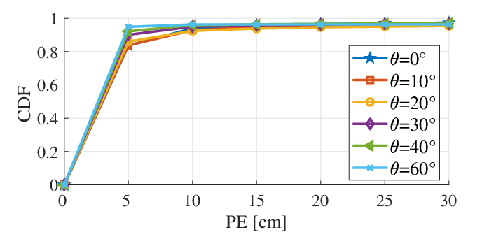
Then, we evaluate the 3D-positioning accuracy of R-P3P with varying tilt angles of LEDs. The performance is represented by the CDF of PEs, given $\theta=0{{}^{\circ}}$, $10{{}^{\circ}}$, $20{{}^{\circ}}$, $30{{}^{\circ}}$, $40{{}^{\circ}}$ and $60{{}^{\circ}}$. As shown in Fig. 5, R-P3P can achieve 80th percentile accuracies of less than 5 cm for all $\theta$. Therefore, R-P3P can be utilized widely in the scenarios where the LEDs are in any orientation. Besides, the accuracy of R-P3P increases slightly as the tilt angle of LEDs increases since the irradiance angles decrease which further improves the received signal power.

2) Effect of the image noise

Since R-P3P also exploits visual information, we then evaluate the effect of the image noise on the accuracy performance of R-P3P, CA-RSSR and the PnP algorithms for 3D positioning under the case where the LEDs tilt with a random angle perturbation $\theta\leq 5{{}^{\circ}}$. The image noise is modeled as a white Gaussian noise having an expectation of zero and a standard deviation ranging from 0 to $4$ pixels [20]. The mean of PEs that are affected by the image noise are shown in Fig. 6. As shown in Fig. 6, the accuracy performance of R-P3P closes to that of the PnP algorithm and is much better than that of CA-RSSR. For R-P3P, the means of PEs increase from 3 cm to 10 cm with the increasing of the image noise. For the PnP algorithm, the means of PEs increase from 0 to 9 cm. In contrast, for CA-RSSR, the means of PEs keeps at about 72 cm.

3) Effect of the distance between the PD and the camera

Since R-P3P exploits the PD and the camera simultaneously, we then evaluate the effect of the distance between the PD and the camera, $d_{\textrm{PC}}$, on the accuracy performance of R-P3P. We compare CA-RSSR and R-P3P on 3D-positioning performance with varying $d_{\textrm{PC}}$ under the case where the LEDs tilt with a random angle perturbation $\theta\leq 5{{}^{\circ}}$. This performance is represented by the CDF of the PEs with $d_{\textrm{PC}}=0\;\mathrm{cm}$, $1\;\mathrm{cm}$, $3\;\mathrm{cm}$, $6\;\mathrm{cm}$ and $10\;\mathrm{cm}$. In particular, $d_{\textrm{PC}}=0\;\mathrm{cm}$ indicates the ideal case that the PD and the camera overlap. As shown in Fig. 7, compared with CA-RSSR, R-P3P can achieve better performance. In specific, R-P3P can achieve 80th percentile accuracies of about 5 cm regardless of $d_{\textrm{PC}}$. In contrast, CA-RSSR can only achieve 40th percentile accuracies of about 30 cm for all $d_{\textrm{PC}}$. As we can observe from Fig. 7, $d_{\textrm{PC}}$ has little effect on positioning accuracy of R-P3P. This means that R-P3P can be widely used on devices with various $d_{\textrm{PC}}$.

In this subsection, we compare execution time of R-P3P, CA-RSSR and the PnP algorithm for 3D positioning to evaluate the computational cost performance [15][22]. To have a fair comparison, all algorithms have been implemented in Matlab on a $1.6\mathrm{GHz}\times 4$ Core laptop. The experiment consists of $10^{5}$ runs. The results are shown in Fig. 8. Since R-P3P estimates the position of the receiver by the LLS method, the computational cost of R-P3P is the lower than that of CA-RSSR, and the execution time of it is shorter than $0.001\>\mathrm{s}$ for almost 100% of the $10^{5}$ runs. Considering a typical indoor walking speed 1.3 m/s, the execution delay of R-P3P only causes 0.2 cm positioning error, which is acceptable for most applications. Besides, the computational cost of the PnP algorithm is over $0.002\>\mathrm{s}$ for about 90% of the $10^{5}$ runs, which means the computational cost of R-P3P is less than 50% of that of the PnP algorithm.

References

- [1] T.-H. Do and M. Yoo, “An in-depth survey of visible light communication based positioning systems,” Sensors 16, 678 (2016).
- [2] P. Pathak, X. Feng, P. Hu, and P. Mohapatra, “Visible light communication, networking and sensing: Potential and challenges,” IEEE Commun. Surveys Tuts. 17, 2047–2077 (2015).
- [3] K. Gligorić, M. Ajmani, D. Vukobratović, and S. Sinanović, “Visible light communications-based indoor positioning via compressed sensing,” IEEE Commun. Lett. 22, 1410–1413 (2018).
- [4] F. Alam, M. Chew, T. Wenge, and G. Gupta, “An accurate visible light positioning system using regenerated fingerprint database based on calibrated propagation model,” IEEE Trans. Instrum. Meas. 68, 2714–2723 (2018).
- [5] T. Q. Wang, Y. A. Sekercioglu, A. Neild, and J. Armstrong, “Position accuracy of time-of-arrival based ranging using visible light with application in indoor localization systems,” J. Lightw. Technol. 31, 3302–3308 (2013).
- [6] Y. S. Eroglu, I. Guvenc, N. Pala, and M. Yuksel, “AOA-based localization and tracking in multi-element VLC systems,” in Proc. IEEE 16th Annu. Wireless Microw. Technol. Conf. (WAMICON), (2015), pp. 1–5.
- [7] L. Wang, C. Guo, P. Luo, and Q. Li, “Indoor visible light localization algorithm based on received signal strength ratio with multi-directional LED array,” in Proc. IEEE Int. Conf. Commun. Workshops (ICC Wkshps), (2017), pp. 138–143.
- [8] L. Bai, Y. Yang, C. Guo, C. Feng, and X. Xu, “Camera assisted received signal strength ratio algorithm for indoor visible light positioning,” IEEE Commun. Lett. 23, 2022–2025 (2019).
- [9] Y. Li, Z. Ghassemlooy, X. Tang, B. Lin, and Y. Zhang, “A VLC smartphone camera based indoor positioning system,” IEEE Photon. Technol. Lett. 30, 1171–1174 (2018).
- [10] L. Wang and C. Guo, “Indoor visible light localization algorithm with multi-directional PD array,” in Proc. IEEE Glob. Commun. Conf. Workshops (GC Wkshps), (2017), pp. 1–6.
- [11] L. Li, P. Hu, C. Peng, G. Shen, and F. Zhao, “Epsilon: A visible light based positioning system,” in Proc. 11th USENIX Symp. Netw. Syst. Design Implement (NSDI’14), vol. 14 (2014), pp. 331–343.
- [12] Z. Yang, Z. Wang, J. Zhang, C. Huang, and Q. Zhang, “Wearables can afford: Light-weight indoor positioning with visible light,” in Proc. Annu. Int. Conf. Mobile Syst., Appl., Serv. (MobiSys ’15), (2015), pp. 317–330.
- [13] M. Rahman, M. Haque, and K. Kim, “High precision indoor positioning using lighting LED and image sensor,” in Proc. 14th Int. Conf. Comput. Inf. Technol. (ICCIT 2011), (2011), pp. 309–314.
- [14] V. Lepetit, F. Moreno-Noguer, and P. Fua, “EPnP: An accurate O(n) solution to the PnP problem,” Int. J. Comput. Vis. 81, 155 (2009).
- [15] L. Kneip, D. Scaramuzza, and R. Siegwart, “A novel parametrization of the perspective-three-point problem for a direct computation of absolute camera position and orientation,” in Proc. 24th IEEE Conf. Comput. Vis. and Pattern Recognit. (CVPR), (2011), pp. 2969–2976.
- [16] T. Komine and M. Nakagawa, “Fundamental analysis for visible-light communication system using LED lights,” IEEE Trans. Consum. Electron. 50, 100–107 (2004).
- [17] Y. Yang, Z. Zeng, J. Cheng, C. Guo, and C. Feng, “A relay-assisted OFDM system for VLC uplink transmission,” IEEE Trans. Commun. 67, 6268–6281 (2019).
- [18] X. Gao, X. Hou, J. Tang, and H. Cheng, “Complete solution classification for the perspective-three-point problem,” IEEE Trans. Pattern Anal. Machine Intell. 25, 930–943 (2003).
- [19] W. Wu, “Basic principles of mechanical theorem proving in geometries,” J. of Sys. Sci. and Math. Sci 4, 221–252 (1984).
- [20] L. Zhou, Y. Yang, M. Abello, and M. Kaess, “A robust and efficient algorithm for the pnl problem using algebraic distance to approximate the reprojection distance,” in Proc. AAAI Conf. Artif. Intell., vol. 33 (2019), pp. 9307–9315.
- [21] K. Cui, G. Chen, Z. Xu, and R. D. Roberts, “Line-of-sight visible light communication system design and demonstration,” in Proc. 7th Int. Symp. Commun. Syst. Networks Digital Signal Processing (CSNDSP), (2010), pp. 621–625.
- [22] J. Lim, “Ubiquitous 3D positioning systems by LED-based visible light communications,” IEEE Wireless Commun. 22, 80–85 (2015).