Non-minimally coupled curvaton
Lei-Hua Liua 11 1 liuleihua8899@hotmail.com and Tomislav Prokopecb 22 2 t.prokopec@uu.nl
a Department of Physics, College of Physics, Mechanical and Electrical Engineering
,
Jishou University, Jishou 416000, China
bInstitute for Theoretical Physics, Spinoza Institute
and the Center for Extreme Matter and Emergent Phenomena (EMME),
Utrecht University, Buys Ballot Building, Princetonplein 5,
3584 CC Utrecht, the Netherlands
Abstract
We investigate two-field inflationary models in which scalar cosmological pertubations are generated via a spectator field nonminimally coupled to gravity, with the particular emphasis on curvaton scenarios. The principal advantage of these models is in the possibility to tune the spectator spectral index via the nonminimal coupling. Our models naturally yield red spectrum of the adiabatic perturbation demanded by observations. We study how the nonminimal coupling affects the spectrum of the curvature perturbation generated in the curvaton scenarios. In particular we find that for small, negative nonminimal couplings the spectral index gets a contribution that is negative and linear in the nonminimal coupling. Since in this way the curvature spectrum becomes redder, some of curvaton scenarios can be saved, which would otherwise be ruled out. In the power law inflation we find that a large nonminimal coupling is excluded since it gives the principal slow-roll parameter that is of the order of unity. Finally, we point out that nonminimal coupling can affect the postinflationary growth of the spectator perturbation, and in this way the effectiveness of the curvaton mechanism.
1 Introduction
In most of inflationary models the inflaton (which drives inflation) is the origin of the curvature perturbation that sources the principal part of the CMB temperature fluctuations. However, viable alternatives exist in which the curvature perturbation is predominantly generated by another scalar field, whose energy density is subdominant during inflation. These models are known as multifield inflationary models with spectator fields, an important class of which was dubbed curvaton scenarios [1, 3, 2].
In curvaton scenarios, the standard relation for the curvaton spectral index, , where is the principal slow-roll parameter, the curvaton mass and the Hubble parameter, yields via its post-inflationary decay a curvature perturbation with a spectral index given by, . Here we consider a simple modified spectator field model in which the spectator condensate couples nonminimally to gravity and observe that the spectator spectral index acquires an additional contribution from its nonminimal coupling of the form, , where is the nonminimal coupling. Since that contribution is , it can be used to tune the spectral index of the spectator field – and thus also via the curvaton mechanism that of the curvature perturbation – which be of the crucial importance for viability of the curvaton model. This simple observation is the principal result of this work.
The nonminimal coupling is not only important during inflation [4, 5, 6], but it can also play an important role for the post-inflationary curvaton decay, which we investigate as well. In most of curvaton scenarios the curvaton decays predominantly perturbatively [7] significantly after the end of inflation. Roughly speaking the decay occurs when the curvaton decay rate becomes comparable to the expansion rate of the Universe , i.e. when . When the assumption that the curvaton condensate dominates over its perturbations is relaxed, the decay process can produce large local non-Gaussianities [8]. Current observations [9] severely constrain these models however, as (local) non-Gaussianity cannot be too large (), thereby ruling out curvaton models that produce large non-Gaussianities.
There are situations where the inflaton does not decay perturbatively, but instead non-perturbative decay channels, such as parametric resonant or tachyonic decay channels [10, 11, 12, 13, 14, 15, 16] are more efficient. The possibility that the curvaton may decay non-perturbatively has also been envisaged [17, 18]. Furthermore, it is known that one can produce a significant amount of gravitational waves during preheating [19]. If the curvaton lives longer, it can couple to the Higgs field in which case the mass of the curvaton can vary significantly [21, 20]. In this work we provide a preliminary analysis of post-inflationary dynamics of two fields after and leave a more complete account of it for future work.
The paper is organized as follows. In section 2 we introduce our inflationary model with two scalar fields, one being the inflaton and the other the spectator nonminimally coupled to gravity. In section 3 we make use of the gauge-invariant two-field formalism to calculate the spectra of the curvature perturbation and entropy perturbation by making use of the general slow-roll analysis. We pay a particular attention to the role of the nonminimal coupling. In section 4 and in appendix B we study how nonminimal coupling influences post-inflationary dynamics and the corresponding spectra of the curvature and entropy perturbations. In section 5 we summarize our main results and discuss some possible future lines of research.
We work in natural units in which , but retain the Newton constant .
2 The model
In this section we consider an inflationary model consisting of two scalar fields, in which one scalar () is the inflaton and the other () is the spectator field nonminimally coupled to gravity. 33 3 Even though we are mainly interested here in a class of two field models of inflation, one of which is the inflaton and the other the non-minimally coupled curvaton field, the formalism we develop applies to the more general situations in which the second field is a spectator field. This more general approach is dictated by the nonminimal coupling, as many of the standard formulas developed in the context of curvaton scenarios do not apply in this more general setting. The action in Jordan frame (denoted by subscript ) is,
| (1) |
where in this work and potential are given by,
| (2) | |||||
| (3) |
where is the reduced Planck mass, is the inflaton potential, is the spectator mass, is its nonminimal coupling and, unless stated otherwise, we take the spectator self-coupling . Next, for simplicity we assume no direct coupling between the inflaton and the spectator. That significantly simplifies our analysis but – unless the mutual coupling is quite strong – in no essential way affects the main results of this work. Furthermore, in this work we work with a simple potential for the inflaton,
| (4) |
even though the precise form of the potential is not important for the purposes of this paper. The exponential potential in (4) is particularly useful since the single field inflationary model in its attractor mode leads to particularly simple slow-roll parameters, , and all other slow-roll parameters are exactly zero (in the attractor mode of the theory), (). Of course, it is important to study other types of inflaton potentials and its interactions with other matter fields, and we leave that for future work. Namely, our main interest here is to study the effects of the nonminimal coupling of the spectator field , and therefore in this work we shall not complicate that by including more complex interactions and further couplings to gravity such as the inflaton nonminimal coupling or the kinetic coupling to the Einstein tensor.
It turns out that a particularly useful frame is the one in which gravity is transformed into Einstein frame, while the inflaton and curvaton are kept in Jordan frame,
| (5) | |||||
| (6) | |||||
| (7) |
After the above transformations are exacted, the action (1) becomes,
| (8) | |||||
where the transformed potential equals,
| (9) |
Note that in the limit of the minimal coupling, , we have and the two fields in (8–9) decouple, implying that this two-field inflationary model reduces to a single field inflation driven by the inflaton which can be treated within the standard slow-roll inflationary framework. For small curvaton condensates the curvaton part of the potential in (9) can be expanded as,
| (10) |
In order to facilitate the analysis, it is convenient to introduce the covariant multifield formalism [22, 23, 26], in which (8) can be recast as,
| (11) |
where is the configuration (field) space metric in (8) which, in the field space coordinates , reads
| (12) |
Note that the field space metric is diagonal. Since the corresponding configuration space curvature tensor does not vanish,
| (13) |
the kinetic terms in the action (11) cannot be brought into the canonical form. It is in this sense that the Einstein frame for the fields does not exist. The dependence of on and the field is illustrated in figure 1, from which we see that, in the limit of large and negative , the configuration space curvature asymptotes to a negative constant , and thus belongs to the class of models with a negative configuration space curvature. These models have gained in popularity, and notable examples are the super-gravity inspired -attractors [27, 28, 29] and the Weyl symmetric models [30, 31].
In the following section we discuss how to calculate the curvature power spectrum under the assumption that the inflaton contribution dominates. While the small field expansion (10) often suffices for rough estimates, it is in general not enough to provide accurate answers for the curvaton dynamics and the respective spectrum of its quantum fluctuations during inflation. For this reason, in what follows we present the analysis by using the full potential (9).
3 Power spectrum
We work in spatially flat cosmological space-times whose background metric is of the form,
| (14) |
where denotes the scale factor and is the lapse function. The expansion of the Universe is driven by field condensates, and , and it is governed by Friedmann equations,
| (15) | |||||
| (16) |
where is the Hubble rate and and denotes the time reparametrization invariant time derivative and are the background fields, which obey [23] 44 4 One can easily show that Eq. (17) is not independent, as it can be derived from covariant conservation of the background stress-energy tensor, and the Friedmann equation (15).
| (17) |
where is the covariant derivative on the field space. Since the background fields are coordinates on the configuration space manifold, the covariant derivative acts simply on the background fields,
| (18) |
where are the Christoffel symbols of the field space. We therefore see that the background fields obey a geodesic equation (17) in presence of a time dependent (Hubble) friction and an external force . 55 5 If one understands , and as , the background equations (15–16) and (17) become time reparametrization invariant, and thus can be easily converted to any other definition of time, e.g. conformal time for which and .
In order to obtain the curvature power spectrum, one ought to solve the operator equation of motion for the curvaton and inflaton, which can be obtained by varying the action (8). When gravitational constraints are solved the linearized equations for field perturbations in the zero curvature gauge 66 6 Since this is a fully fixed gauge, the equations (19) are identical to the equations of motion for the corresponding gauge invariant variables in the zero curvature gauge, in which reduces to the field perturbations . For a more detailed discussion of this issue see, for example, Refs. [24, 25]. are [23],
| (19) | |||
where , , the Riemann tensor is given in (13) and
| (20) | |||||
| (21) |
such that
| (22) | |||||
where we made use of Eq. (17) and of,
| (23) |
The nonvanishing Christoffel symbols are,
| (24) |
The next natural step is canonical quantisation, according to which the fields and their canonical momenta
| (25) |
satisfy canonical commutation relations,
| (26) |
while the fields and their canonical momenta mutually commute. Perturbations around the field condensates satisfy identical commutation relations as in (26). This can be seen by expanding the action (8) to the quadratic order in perturbations, including the effect of coupling to the gravitational perturbations. The resulting action can be found e.g. in Ref. [32] (see Eq. (4.19)) (for a discussion of more general multifield Lagrangians see Ref. [33]), from where it is clear that coupling to gravity does not change the structure of the canonical kinetic term, such that the canonical quantization relation (26) holds also for the perturbations,
| (27) |
where .
Since the procedure for studying the dynamics of quantized linear curvature perturbations is standard [34], here we outline just its main steps. The quantum fields that exhibit kinetic and potential mixing (which are both evident from (8–9) and (19)) can be decomposed into spatial momentum modes as,
| (28) |
where are matrix valued mode functions, and are the creation and annihilation operators in the instantaneously diagonal basis denoted by the intex , which obey,
| (29) |
The spectra of different field components can be then defined as,
| (30) |
where the normalization of the modes can be determined from the Wronskian,
| (31) |
where are the canonical momenta associated with the mode functions .
These quantities are, however, not directly observable. In order to reach observable spectra, it is convenient to define the curvature and entropy directions in the field space as follows,
| (32) |
such that the norm of the entropy vector is unity, . In terms of these quantities the background Friedmann equations (15–16) simplify to,
| (33) | |||||
| (34) |
and the background field equation (17) for the adiabatic mode becomes identical to that of one field inflation,
| (35) |
where . Note that, just as in the one field case, Eq. (35) can be derived from Eqs. (33–34) by taking a time derivative of (33). Eqs. (34) suggest the following definition of the principal geometric slow-roll parameter,
| (36) |
By projecting Eq. (19) onto , one can then show that the equation of motion for reads,
| (37) |
where
| (38) |
is the mass term of the adiabatic perturbation and
| (39) |
defines the turning rate, which is by definition orthogonal to , , and can be used to define convenient orthonormal basis vectors for the perturbations. Indeed, we can define a unit turning vector as,
| (40) |
which can be used to project out the entropy perturbation,
| (41) |
Note that since are orthogonal, the adiabatic and entropy (or isocurvature) perturbations, , denote the two orthogonal perturbations (since we have only two fields, this completes the procedure of diagonalization of the perturbations).
Since the projection vectors and are orthonormal, from (27) one can infer that the nonvanishing canonical commutation relations for and are,
| (42) |
where and . Notice also that, as a consequence of orthogonality, , the remaning commutation relations vanish, e.g. , which is true in spite of the mixing of perturbations in (37).
The effective mass in the evolution equation (37) for the adiabatic perturbations does not depend on the configuration space curvature (which drops out due to a Bianchi identity), but it acquires a negative contribution from the turning rate . Note also that the source on the right hand side of (37) is entirely due to the entropy perturbation .
The entropy perturbation obeys, 77 7 Since we are considering here only the two fields case, our equation for the entropy perturbation (43) is simpler than the more general one presented in [23], which holds for general multifield case.
| (43) |
where the mass term and the curvature contributions read,
| (44) |
and is the Bardeen’s spatial (gauge invariant) potential. Note that – unlike in the case of the adiabatic perturbation – the turning rate contributes positively to the mass term of the entropy mode (see, however, Eq. (53) below). Furthermore, while in the adiabatic mode equation the configuration space curvature does not contribute, it does contribute to the mass of the entropy perturbations as, , which is positive (negative) for a negatively (positively) curved configuration space manifold.
The equations for the perturbations (37) and (43) can be closed by making use of the relation between the Bardeen potential and the curvature and entropy perturbations,
| (45) |
where, in the last step, we used the following relations between the curvature perturbation and the entropy perturbation and the variables and ,
| (46) | |||||
| (47) |
and we have introduced the second geometric slow-roll parameter,
| (48) |
Next, it is convenient to introduce the directional curvature and entropy covariant derivatives as,
| (49) |
Of course, if and act on a scalar quantity once, they act as ordinary derivatives, and we shall denote them to indicate that, i.e. and . Armed with these, one can show that in (38) can be rewritten as,
| (50) |
where we made use of (39–40) and of
| (51) |
This equality follows from (39) and can be used to determine the sign of .
Upon making use of (44–45) and (50) in (37) and (43) we obtain the following equations,
| (52) | |||||
| (53) |
where we made use of,
| (54) |
and its directional derivative, , 88 8 Since is a scalar quantity, we then have .
and we have converted, when possible, to slow-roll parameters. Notice that the form of the equation for the curvature perturbation (52) is such that the only difference between the corresponding one field equation and (52) is that, in the multi-field case, the curvature perturbation is sourced by the entropy perturbation, whose precise form is shown on the right hand side of (52). The structure of Eqs. (52–53) reveals that and decouple when the turning rate . From Eq. (54) we see that this will be the case if the directional dervative of along vanishes. Alternatively, will vanish if is time independent, which will be approxuimately the case if is dominated by the inflaton kinetic energy, i.e. if . In practice that will be the case if and if the curvaton condensate is small enough, .
In view of (46–47), equations (52–53) can be easily converted into equations for and ,
| (55) | |||||
| (56) |
where
| (57) |
As one could have expected, the mass term () has completely disappeared from the equation for the curvature perturbation , which must be so also in the multifield case. What is also interesting is that the same operator as it acts on , acts in the source on . Upon rewriting (55) as,
| (58) |
we see that, on super-Hubble scales, on which , the following quantity is conserved,
| (59) |
where we introduced the number of e-foldings, (). This means that the (rate of change of the) curvature perturbation on super-Hubble scales is given by,
| (60) |
where is chosen such that the gradient term on the right hand side of Eq. (58) can be neglected, which is the case when evaluated at is sufficiently small when compared with unity. Hence, in order to calculate the spectrum of the curvature perturbation, we need to know how the entropy perturbation evolves in time. Since Eq. (56) cannot be solved in general, we shall solve it in slow-roll approximation, which is what we do next.
3.1 Slow-roll analysis
Equations (55–56) are easy enough such that they can be analyzed in slow-roll approximation. We shall perform our analysis in two steps. In step 1 we determine the spectra at a scale close to the Hubble scale. This analysis can be done at the leading (zeroth) order in slow-roll parameters, but the gradient operators must be kept. In step 2 we shall study the evolution of the curvature perturbation on super-Hubble scales induced by the entropy perturbation, again to the leading order in slow-roll approximation. While this analysis is guaranteed to correctly reproduce the spectra and spectral indices to the leading order in slow-roll parameters, because of the coupling between the fields, potentially interesting features may be hidden in the subleading results for the spectra. For that reason in Appendix A we analyze the spectra at the subleading order in the slow-roll parameters and find that the curvature-entropy spectrum is generated at the next-to-leading order in the slow-roll parameters (its amplitude being proportional to the turning rate ), even if at the beginning of inflation this correlator was set to zero.
Step 1. Observe firstly that at the zeroth order in slow-roll, Eqs. (55–56) simplify to,
| (61) | |||||
| (62) |
where we made use of the fact that the coupling between the perturbations is suppressed by the turning rate, , which we assume to be suppressed in slow-roll approximation, i.e. .
Since the perturbations decouple, it is easy to solve Eqs. (61–62). When written in terms of (conformal) time, , Eqs. (61–62) become,
| (63) | |||||
| (64) |
where and is the conformal expansion rate, which in this approximation is simply, (). In order to obtain the spectra on the sub-Hubble scales, one ought to solve the quantum version of (63–64), i.e. one ought to promote and to operators, , , which satisfy the following canonical commutation relations (),
| (65) |
and all other commutators vanish. Here we have introduced canonical momenta,
| (66) |
where these relations follow from the canonical momenta and in Eq. (42). Upon transforming into the spatial momentum space (cf. Eq. (28)), from (62) we obtained the mode equations and (),
| (67) |
which can be solved in terms of the Hankel functions with the index, . The normalization can be determined (up to Bogolyubov transformations) from the Wronskian conditions (cf. Eq. (31)),
| (68) |
Notice that here the mode functions are ordinary functions, which is to be contrasted with the general case (28), in which they are matrix valued. Here we make the simplest – positive frequency – choice of the vacuum (also known as the Bunch-Davies or Chernikov-Tagirov vacuum), and we obtain,
| (69) |
These short-wavelength solutions can be inserted into the standard formulas for the spectra,
| (70) | |||
| (71) |
which are valid up to mildly super-Hubble scales (on which with and ). Upon inserting (69) into (70–71) we obtain,
| (72) |
where we neglected the conformal parts, which come as a multiplicative factor in (72), which is justified on super-Hubble scales. The solutions (72) are correct up to the leading order in slow-roll parameters. One can construct slow-roll corrections to these solutions by solving the full equations (55–56) iteratively in powers of slow-roll parameters, e.g. by using the method of Green’s functions. The resulting corrections are slow-roll suppressed when compared with the leading results (72). The details of such an analysis can be found in Appendix A. The spectral indices in (70–71) are then obtained in the standard manner, by taking a derivative with respect to and setting it to the Hubble crossing scale, . The result is, to leading order in slow-roll,
| (73) |
where all quantities are evaluated at a fiducial scale , with . This completes our analysis of short scales.
Step 2. As we have shown in Eq. (60) above, in the two field case the curvature perturbation is not constant on super-Hubble scales, but it is sourced by the entropy perturbation, which in turn can modify its spectrum. In order to make progress, in what follows we shall solve the evolution equations (55–56) on super-Hubble scales, but now keeping the linear slow-roll corrections.
Indeed, when the entropy field mass 99 9 The opposite limit, when is rather easy, since in this case one can use adiabatic approximation to solve for the mode functions of the entropy perturbation. Since in this case the effect of the entropy perturbation on the curvature perturbation is expected to be small on super-Hubble scales, this case is trivial and we do not consider it any further. and the turning rate are small, i.e. when,
| (74) |
both satisfied, then the source on the right hand side of (56) can be approximated by, , such that, on super-Hubble scales, Eq. (56) simplifies to,
| (75) |
Since the last term on the left hand side is suppressed by , and is typically of the order unity or smaller, all terms contributing to the effective mass of the entropy perturbation are suppressed (at least linearly) by slow-roll parameters. Notice next that the form (75) of the equation for the entropy perturbation follows immediately from Eq. (43), in which the source on the right hand side is suppressed by the Laplacian of the Bardeen potential, and hence can be neglected on super-Hubble scales. Equation (75) tells us that on super-Hubble scales approximately decouples from , implying that one can first solve (75) for the entropy perturbation, and then insert the solution into the equation for the curvature perturbation (60) to get the desired spectrum.
To the leading order in slow-roll parameters and on super-Hubble scales Eq. (56) simplifies to,
| (76) | |||||
where is a derivative with respect to the number of e-foldings (defined by ) and we kept only the leading (linear) order terms in slow-roll ( is of higher (second) order in slow-roll). Eq. (76) can be easily solved,
| (77) |
which tells us how evolves on very large scales, where . This evolution results in an additional contribution to the spectral index (cf. Eq. (73)) 1010 10 One can show that the spectral index of the entropy perturbation is twice the derivative with respect to the Hubble crossing time, of the exponent of the solution given in (77) which is, to leading order in slow-roll, equal to the derivative with respect to . of the form,
| (78) |
where all parameters in (78) are evaluated at . In fact, evaluating these quantities at a different time is permitted, since that would lead to a result that differs at higher order in slow-roll, and thus is immaterial for the present analysis.
We are now ready to consider the adiabatic perturbation. Integrating Eq. (60) and neglecting the first term (which amounts to neglecting the decaying mode), we obtain,
| (79) | |||||
where, to get the last result, we made use of and we have introduced the transfer function for the entropy perturbation (see (77)) ,
| (80) |
Now upon taking derivative of the logarithm of (79) with respect to , multiplying by 2 and making use of (80), we get the following contribution to the spectral index of the adiabatic perturbation due to its coupling to the entropy perturbation,
| (81) |
Several remarks are now in order. The entropy perturbation can through Eq. (80) contribute to the curvature perturbation. Unless the transfer function is quite sizable, the contribution in the denominator of (81) can be neglected as it is suppressed by the slow-roll parameter . Notice also that, even though the exponent of the transfer function in (80) is suppressed by slow-roll parameters, it is not necessarily small because of the integral, which produces an enhancement by a factor . For sufficiently late times , such that it can compensate the smallness of the slow-roll parameters. For that reason it is important to keep that term in Eq. (81) even though naîvely one would be tempted to conclude that it contributes at a higher order in slow-roll parameters. Furthermore, the sign of the exponent in (80) is important. Namely, if the sign of the integrand is positive (negative), the transfer function decreases (increases) in time, which in turn implies that the contribution of the entropy perturbation to the spectral index decreases (grows) in time, rendering the curvature spectrum bluer (redder).
To conclude, the principal results of this section are formulas (72) and (70) for the spectrum of of the adiabatic and entropy perturbation, with the spectral indices given in Eqs. (73), (78) and (81) which, when summed, yield,
| (82) | |||||
| (83) |
There is also the mixed correlator, , whose amplitude is suppressed by the turning rate , see Eq. (197), and since the turning rate is typically small (it is suppressed by the slow-roll parameter ) its amplitude is suppressed when compared with that of the curvature and entropy correlators. Its spectral index is simply, . Unless either the turning rate or the transfer function is rather large, the contribution of the ratio in (82) can be approximated by unity. In this case the adiabatic spectral index simplifies to,
| (84) |
such that the principal contribution of the entropy perturbation to the spectral index of the curvature perturbation, , comes from the turning rate (expressed in units of ). When () the coupling to the entropy perturbation reduces (enhances) the spectral index in (84), such that the corresponding spectrum becomes redder (bluer). While the curvature spectrum gets a correction from the entropy perturbation through the transfer function in (79), this correction is typically small and can be neglected, unless either the turning rate or the transfer function is quite large. More precisely, when and and change adiabatically slowly in time, then the spectrum of the curvature perturbation (82) can be approximated by,
| (85) |
which in the limit approaches that of the single field inflation. What is also interesting in Eqs. (84) and (83) is that, while the configuration space curvature contributes to the spectral index of the entropy perturbation, it does not contribute to the spectral index of the curvature perturbation.
3.2 Explicit form for slow-roll parameters
In this subsection we give explicit forms for the slow-roll parameters. The Hubble parameter and the principal slow-roll parameter are given by (to leading order in derivatives),
| (86) |
The higher order slow-roll parameters are,
| (87) | |||||
| (88) | |||||
where the last term in (88) equals to .
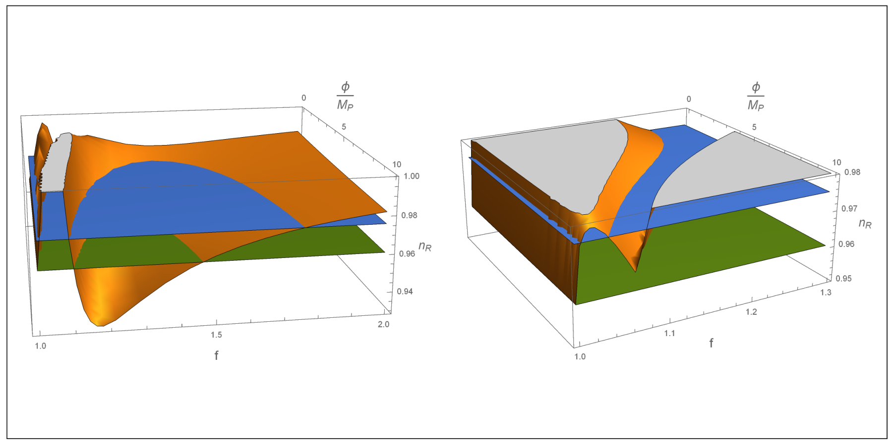
Based on the above expressions in figure (2) we plot the spectral index of the curvature perturbation (red surface) which, in the limit of a small transfer function (i.e. a small turning rate ), can be well approximated by (84). The lower and upper Planck collaboration limits on the scalar spectral index, , are also shown (green and blue horizontal planes, respectively). The spectral index is shown as a function of (horizontal axis) and (the axis pointing into the paper) and the noniminimal coupling. We see that the values which are consistent with the observations typically corresponds to in the range from 1 to 2 and rather small, negative nonminimal couplings. The value of is not very relevant, since for the exponential inflaton potential we consider in this work (4), a shift in can be always compensated by a multiplicative change in .
Next we need is the unit vectors and and the turning rate (39). From (32) we know that , which in slow-roll approximation becomes,
| (89) |
To get the turning rate , one inserts the slow-roll result (89) into the definition (39) to obtain,
| (90) |
where we made use of and . Eq. (90) then immediately implies,
| (91) |
In figure 3 we illustrate how defined in (91) and (90) depends on the curvaton field condensate and on the nonminimal coupling . The generic trend is that the turning rate peaks at a rather small field value, (), and then decays as increases. Furthermore, the peak value of increases as increases, which means that the coupling between the curvature and entropy perturbations becomes stronger, as can be seen from e.g. Eq. (55).
The unit turning vector is formally,
| (92) |
where . While this expression is formally correct and can be used to construct , there is an easier way to proceed, namely to use and , which uniquely fix it to,
| (93) |
Even though this expression looks noncovariant, it is in fact covariant, as its covariant form is given by (92). It is nevertheless simple, and thereby convenient to use in practical calculations.
Next, we need a slow-roll expression for defined in (44), or equivalently the corresponding slow-roll parameter . Making use of (92) and (90), after some algebra, one gets,
| (94) | |||||
where the denominator comes from multiplying by .
Next, from equation (83) we also need contribution from the configuration space curvature,
| (95) |
where we made use of (86) and (13). When (for which ), the curvature term (95) contributes positively to the spectral index of the entropy perturbation.
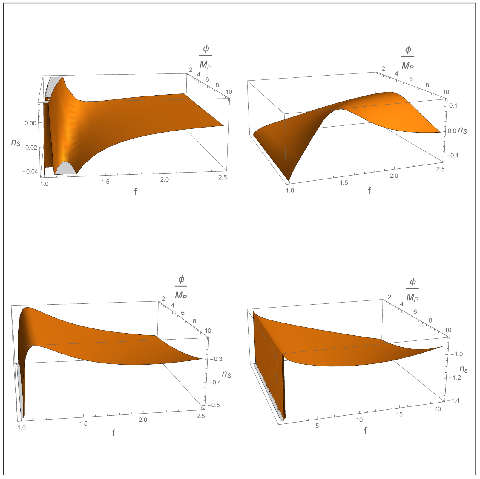
Figure 4 shows four panels illustrating the spectral index of the entropy perturbation defined in Eq. (83) as a function of the curvaton and inflaton condensates. The four panels illustrate the dependence of the spectral index on the nonminimal coupling . The general trend is that the spectral index becomes more negative as becomes more negative, indicating that the spectrum of the entropy perturbation grows faster on very large scales, which means that the entropy perturbation dominates over the curvatre spectrum of the single field adiabatic model. When combined with the observation that also the turning rate (90) grows with increasing (see figure 3), this suggests that, as becomes more and more negative, the energy between the entropy and the curvature perturbations gets more efficiently transferred. However, there are limitations on how large can be since – as we argue below – cannot be much larger than unity. A detailed study of the precise consequences of these crude observations we leave for future work.
Finally, in order to evaluate the transfer function (80) (see also (81)), we need to integrate slow-roll suppressed terms over the number of e-foldings . The number of e-foldings can be expressed in slow-roll as,
| (96) |
where is used as the clock during inflation. Inflation ends at a point when,
| (97) |
However, these formulas are not useful as long as we do not have an explicit expression on how the fields depend on the number of e-foldings, . In what follows we use the slow-roll relation, , to obtain,
| (98) |
This expression can be, at least in principle, used to obtain the functional dependence of how depends on the fields . For completeness, we shall also derive a relationship that allows to express . Starting with and , one can quite straightforwardly derive the desired expression,
| (99) |
which is rather complicated. Together with (98), this equation allows for construction of the curvilinear coordinates from the original field coordinates . The advantage of using (or equivalently ()) is that these coordinates have a direct physical interpretation: the number of e-foldings can be used to measure time in inflation and (from ) to signal the end of inflation, while can be used to measures the distance between neighboring inflaton trajectories. Finally, in the context of formalism, can be used to study the spectrum of cosmological perturbations.
The expression (98) defines the metric along which the fields move with the number of e-foldings chosen as proper time, i.e. it defines in slow-roll approximation. In general, it is hard to integrate (98), as mixes and ,
| (100) |
where is the potential in Einstein frame (9) and we made use of
| (101) |
To make progress, it is useful to expand (100) for small and for large . First recall that we are interested in the curvaton model, in which , such that upon making use of,
| (102) |
we get the following simplified expression for (100),
| (103) |
This expression can be further simplified by taking the limit and assuming ,
| (104) |
When in addition, is satisfied, further simplifies to . When combined with the constraint on the tensor-to-scalar ratio, and assuming that the one-field inflation relationship holds, , this gives an upper limit on the coupling, (valid if ). Inserting (104) into (98) gives,
| (105) |
where we used the expanded configuration space metric (12),
| (106) |
One can think of the problem of finding as being equivalent to a curved space-time with a configuration space metric,
| (107) |
We shall refer to as a slow-roll metric. Since (107) does not depend on , is a Killing vector, implying a conserved configuration space momentum in the direction, 1111 11 Notice that the naîve configuration space momentum, is not conserved due to the nonvanishing gradient of the potential and the configuration space curvature.
| (108) |
where the sign of is chosen such that when is positive. This is a convenient choice when early in inflation both of the field condensates are positive. For definiteness, here we assume that to be the case. Since the potential and the nonminimal coupling function are symmetric under the exchange of the field sign, the results for the other three cases can be easily obtained from the case studied here. This conserved momentum can be used to convert (105) into an ordinary differential equation for ,
| (109) |
where the sign is chosen such that, as decreases, increases. Since during inflation decreases, will increase. From Eq. (105) we see that the opposite sign choice is allowed, and it corresponds to measuring the time lapse from the end of inflation backwards in time. Since Eq. (109) is hard to integrate in general, we shall make simplifying assumptions, namely that is sufficiently small to satisfy,
| (110) |
and that the conserved momentum is small, i.e.
| (111) |
To estimate , recall first that in the limit when and , the principal slow-roll parameter (104) can be well approximated by, and . When this is inserted into (108) one obtains,
| (112) |
where we neglected the factor . This tells us that inequality (111) is marginally satisfied. At a first sight it seems strange that our estimate (112) of depends on and therefore it does not seem conserved. The explanation is in our inexact (slow-roll) estimate of .
When keeping only the linear quantities in the perturbations and , the integral of (109) simplifies to,
| (113) | |||||
where we neglected the terms that are quadratic and higher order in the perturbations (110–111). This then implies the following expression for ,
| (114) | |||||
where is the same function of as given in the square brackets in (114) with .
In what follows, for simplicity we give expressions to the leading (zeroth) order in the perturbations and . If needed, one can always go back to (114) to iteratively include the linear (and if desired higher) order corrections in the perturbations. Eq, (114) can be inverted to yield 1212 12 By making use of , can be pulled out of the tangent in Eq. (116) to arrive at, (115)
| (116) |
Since , , as it should be. From (108) we can get ,
| (117) | |||||
| (118) | |||||
Notice that, if , then is constant, implying that is the principal cause for to roll. It is interesting to observe that such a trajectory exists. In order to get a better idea on understanding of what the solutions (116) and (118) convey, it is useful to consider the following two limits, early times when , and late times (close to the end of inflation) when which, in the limit when , reduces to . In the former case the following approximation can be used for the tangents in (116) and (118),
| (119) |
with the help of which one obtains,
| (120) | |||||
| (121) |
In the latter limit (when ) one gets,
| (122) | |||||
| (123) | |||||
This suggests that inflation ends when , at which point the number of e-folds reaches, and reaches the value given by the first line in Eq. (123). The more accurate statement is that this two field slow-roll inflation ends e-foldings earlier than that, at which point the field enters a fast roll regime and oscillates around (). The two field inflation ends there and one enters an approximately one field inflation, during which the slow-roll parameters approach, and all higher ones vanish, (), such that inflation never ends. One way to terminate inflation is to add a small mass term for , which creates a local minimum in the potential of , such that the field starts oscillating around that minimum, thus ending inflation.
The solutions (116) and (117) (or their improved versions that include corrections to some order in the perturbations and ) can be used in (80) and (79) to obtain the transfer function for the entropy perturbation as well as the evolution of the adiabatic perturbation on super-Hubble scales due to its coupling to the entropy perturbation. Furthermore, one can obtain the spectral index for the curvature perturbation (81). Since in general such evaluations involve complicated integrals that cannot be dealt with analytically, we leave these for future study.
Let us now consider large limit. In this case Eq. (103) reduces to,
| (124) |
where we again assumed the inflaton dominance, . Note also that, in this limit the Ricci curvature scalar of the configuration space (13) is negative and constant, 1313 13 One can easily show that the configuration space metric in the limit of can be reduced to that of the Poincaré plane, where . The corresponding Ricci scalar is equal to , and thus constant and negative.
| (125) |
This means that negative configuration space curvature prevents inflation from happening (it makes the inflaton potential too steep). This can be rigorously shown by transforming to the frame in which the configuration space metric is of the form, (see Ref. [31] for details). The leading order behavior in the potential for large field values is then , which corresponds to a coupling , and the corresponding . It is interesting that the same asymptotically late time is reached in inflationary models in Einstein frame driven by a cosmological constant and studied in [43].
To summarize, we have analyzed the two-field inflationary model with a nonminimally coupled spectator field and found that, a large nonminimal coupling induces a large negative curvature of the configuration space manifold, such that the principal slow-roll parameter , which is too large to be of interest for inflationary model building. On the other hand, the model is viable when the nonminimal coupling is small. In what follows we analyze this model in a post-inflationary setting. In particular we discuss how cosmological perturbations evolve in radiation and matter era.
4 Post-inflationary dynamics
Here we consider several plausible scenarios for the evolution of scalar cosmological perturbations after inflation, with the principal goal to clarify the role of the nonminimal coupling. Not all of the scenarios correspond to the traditional curvaton scenario, but instead some belong to the more general class of two-field inflationary models. Recall that post-inflationary dynamics is very weakly constrained by the current data, leaving us with numerous theoretical possibilities. For simplicity, here we shall keep track of post-inflationary evolution of the scalar cosmological perturbations on super-Hubble scales only. At linear order the graviton and scalar pertubations decouple, such that tensor cosmological perturbations obey the usual post-inflationary dynamics (their amplitude remains frozen on super-Hubble scales), and we shall not discuss them any further here.
In the former section we analyzed slow-roll dynamics of scalar cosmological perturbations in a two-field inflationary model. We transformed to the more natural basis spanned by the comoving curvature perturbation and the isocurvature (entropy) perturbation . Our principal results are given in Eqs. (70–72) and (82–83). Assuming that the fields (and the corresponding spectra) at the end of inflation (more precisely, at the end of the slow-roll regime) are known and given by , (, with ), in what follows we discuss how to evolve them through post-inflationary epochs. Before we begin our analysis, we note that, at the end of inflation, one of the two different possibilities can be realized:
-
Weak coupling regime. In this regime, the curvature and entropy perturbation couple weakly during inflation (in the sense that the turning rate is small), such that during inflation there is no significant power transfer between the entropy and curvature perturbations, resulting in the usual one-field estimate for the spectra, , , see Eqs. (82–83). The last term in comes from non-canonical structure of the kinetic terms, and can be conveniently expressed by making use of the configuration space curvature .
-
Strong coupling regime. The entropy perturbation couples strongly to the curvature perturbation, such that power transfer between the two spectra is efficient during inflation, resulting in a modified spectrum of the curvature perturbation given in Eq. (82).
Precisely these two regimes can be identified also during preheating and the subsequent radiation and matter epochs, the only difference being that the power transfer between the entropy and curvature perturbations continues after inflation, and thus ought to be taken into account in the final estimate of the curvature spectrum. The latter scenario – the one in which a significant power gets transferred from onto after inflation – corresponds to the usual curvaton scenario, in which the late time comoving curvature perturbation inherits the spectrum of the entropy perturbation. We emphasize that our analysis goes beyond that of the standard curvaton scenario, and since in the multi-field scenario considered in this work the curvature perturbation is not generally conserved on super-Hubble scales, the effects of the coupling between the fields must be carefully studied in order to get a reliable prediction for the spectrum of scalar cosmological perturbations observed in the late time Universe. While the general problem is beyond the scope of this work, in what follows we make a crude analysis of the postinflationary evolution in this model.
Since the perturbation spectra are frozen on super-Hubble scales, the spectral indices of both entropy and curvature perturbations are inherited from the end of inflation. The relevant equations of motion in the postinflationary regime are therefore (58) and (75), which after inflation simplify to,
| (126) | |||||
| (127) |
with initial conditions given by,
| (128) |
When writing Eqs. (126) and (127) we assumed that , which is approximately true during preheating (during which or ) and in radiation era, in which , after preheating is completed. In this work we shall not take into account the time dependence in , which can be significant during preheating after inflation. To see that, recall that during preheating, , where the kinetic energy in the adiabatic mode can exhibit a relatively strong dependence on time.
For the modes of physical interest the decaying mode of has decayed by the end of inflation, such that (126) can be easily solved (cf. Eq. (60)),
| (129) |
Even though Eq. (127) cannot be solved exactly, one can make progress assuming that and that the parameters , and evolve adiabatically in time (in the sense that they do not change much during one expansion time). In this case Eq. (127) is approximately solved by,
| (130) |
where
| (131) |
where we ignored corrections of the order , which are of a higher adiabatic order. When writing (131) we have assumed that is small at the end of inflation (), such that its contribution to the postinflationary can be neglected.
In order to see whether there can be an appreciable transfer of power between and , we need the conditions for not to decay (significantly) after inflation. From (131) we see that that is the case when , or equivalently when ; in other words when , or , or both. For example, if , then and Eq. (130) reduces to, , which is valid both when is positive or negative. When , and and can grow very fast. Finally, when , is complex and there are two oscillatory solutions with the frequency and their enveloping amplitude decays as, , such that rapidly decouples from .
Configuration space curvature. The contribution to in (131), which is simplest to estimate, is that from the configuration space curvature,
| (132) |
where we assumed that after inflation the condensate is small when compared with the Planck scale, such that is a good expansion parameter. This contribution is negative, and in radiation (matter) era it equals four (three) times . If this contribution dominates will grow, thus providing an efficient mechanism for the transfer of power between and , underlying the importance of nonminimal coupling for the curvaton mechanism. There are two other potentially important contributions to in (131), and before we reach any conclusion regarding effectiveness of the curvaton mechanism after inflation, we ought to estimate them.
The turning rate is defined in (51) in terms of the directional derivative of , , where
| (133) |
To make our analysis simpler, in what follows we assume that after inflation the field condensates are sub-Planckian,
| (134) |
Our analysis in appendix B shows that after inflation the fields oscillate with a decaying envelope such that, if (134) is met at the end of inflation, it will be satisfied throughout the postinflationary epochs. The approximate solutions to the equations of motion are given in Eqs. (211–212) and (213–214). From these, one can easily obtain the two basis vectors (cf. Eqs. (32) and (39)),
| (135) |
where . These then imply the following expression for the turning rate
| (136) |
To get a better idea on how large is, we shall calculate it in two limits: (a) when and (b) when . In the former case, provided there is no large hierarchy between the masses of the two fields, , , such that and
| (137) |
where is defined in (209) and
| (138) |
where is assumed. From these expressions we see that oscillates around zero with a typical amplitude,
| (139) |
such that it is suppressed by . Even though it is suppressed, the turning rate may be significant if in (139) is larger than the expansion rate . From (138) we also see that blows up when , which is when is an integer. This is however an artifact of the approximations we used to get to (137). Indeed, by using the more accurate formula (136) one sees that at these special points grows at most to a value, , which is large, but (at least it is) finite. During the short intervals when is relatively large, the coupling between the two fields becomes strong, and may lead to an efficient transfer of power between the entropy and curvature perturbation. We intend to explore the physical ramifications of this interesting effect in the future. For now we just note that the typical turning rate after inflation (139) is small, and thus the transfer of power between the two fields will typically be not inefficient.
Before continuing our analysis, note that there is a simple approximation for , which acquires a particularly simple form when or . However, a constant value of is attained only when the condensates have decayed sufficiently such that is dominated by the plasma contribution, in which case, , where and are the pressure and energy density. But as long as the condensates dominate the energy density and pressure, the pressure (and therefore also ) oscillates, which in turn causes short periods of strong coupling between the curvature and entropy perturbation.
The mass parameter for the entropy perturbation (44) can be approximated by,
| (140) |
where we used the fact that the condensate amplitudes are much smaller than the Planck scale. If in addition , one easily gets,
| (141) |
Upon combining (132), (136–138) and (141) we get for the mass parameter (131) of the entropy perturbation (cf. Eq. (127)),
| (142) |
where we kept unspecified. We did that because, even though is typically small (139), it can vary a lot with time, as can be seen from Eqs. (137–138). From Eqs. (130–131) we know that the entropy perturbation can grow after inflation only if , which implies the following condition on ,
| (143) |
Since oscillates, at some instances when it goes through zero, the condition (142) becomes weaker,
| (144) |
When the condition (143) is satisfied, will grow, 1414 14 The entropy perturbation will likely grow also when the milder condition (144) is satisfied, but to establish that rigorously one would have to analyze Eq. (127) with varying non-adiabatically in time, in which case may exhibit a resonant growth. A complete analysis of this case is beyond the scope of this work. such that, when it later decays, it can imprint its power onto the curvature spectrum with the spectral index given by (83). If that contribution dominates its amplitude, the curvaton mechanism will be effective, and the observed scalar spectrum will be of the form (83). In the simple case when the amplitude of is small enough, i.e. , the spectral index of can be approximated by,
| (145) |
such that when (143) is satisfied, which is what is required by the observations. One can see this by recalling the observational bound on the tensor-to-scalar ratio , which in the case when the one-field inflation consistency relation approximately applies, , from which one sees that the contribution in (145) is not large enough to explain the spectral index in the observed scalar spectrum, whose deviation from scale invariance is approximately, . However, in many curvaton models the tensor-to-scalar ratio is suppressed due to the additional curvaton contribution to the curvature perturbation, such that the observed limit represents a weaker constraint on , which can also help to make the curvaton perturbation (145) redder, underlining yet another advantage of curvaton models. Notice further that adding a large enough negative nonminimal coupling which satisfies (144) can make the spectrum of the entropy perturbation red enough to be consistent with the observed value of . When this is combined with condition (143), one sees that, the same condition which reddens the spectrum of the entropy perturbation, induces its postinflationary growth. When combined with an efficient transfer of power (which can be facilitated either by a strong enough linear coupling or by the decay of entropy perturbations typically mediated by some quantum loop process), one can activate the curvaton mechanism.
Since the analysis performed in this section concerns the deep infrared, super-Hubble modes, they will all be amplified by an equal factor (with the caveat that each of the two fields can get amplified by a different factor). That means that the spectra inherited from the end of inflation will not change by the postinflationary evolution. What can happen is that, as the result of the coupling between the perturbations, the spectrum of the entropy perturbations gets imprinted onto the curvature perturbation, such that its spectral index becomes that of the curvature perturbation from the end of inflation. Therefore, this scenario constitutes the two-field variant of the curvaton scenario.
In the above analysis we did not invoke any formulas from the standard curvaton scenario, since they assume that the formalism applies, in which the coupling between the curvaton and inflaton is small and plays no role such that not significant coupling between the two fields is allowed. However, nonminimal couplings induce a coupling between the field perturbations, which in turn can induce a non-negligible transfer of power between the perturbations, invalidating the formalism.
To conclude, the analysis performed in this section shows that a nonminiml coupling of the curvaton field can have a profound impact on the validity of curvaton scenarios. In particular, it can make viable those curvaton models which in their minimal coupling incarnation would be ruled out.
5 Conclusion
In this paper we investigate in some detail a two-field model of inflation in which one of the fields is nonminimally coupled. A particular attention is devoted to the case when the nonminimally coupled field is the curvaton. Models with nonminimally coupled fields are important to study, especially when one recalls that nonminimally coupled scalars are ubiquitous. This is so because, even if nonminimal couplings are set to zero at the classical level, they will be generated by quantum effects, as they induce a running of the nonminimal coupling as long as it is different from its conformal value, .
The principal finding of this work is the observation that a nonminimal coupling can help to keep alive a class of curvaton models that otherwise would be ruled out by observations. Namely, a small negative (positive) nonminimal coupling makes the spectral index of scalar cosmological perturbations redder (bluer), thus counteracting a positive mass term that alone would make the curvaton mass term positive.
In this work we adapt the two field formalism of references [22, 23] (there are earlier references as well), in which one studies scalar cosmological perturbations by rotating into the frame of curvature and entropy perturbation, where the curvature perturbation is the one that directly (at the linear level) couples to gravitational perturbations. The two fields couple by the parameter known as the turning rate defined in (39) and (51). In section 3 we perform the general analysis of our two field model in slow-roll regime. Our results for the spectral indices for the curvature and entropy perturbations are given in Eqs. (82) and (83), from where one sees that the spectral index of the curvature perturbation is influenced by the turning rate and by the transfer function (defined as the ratio of the entropy and curvature perturbation), such that for positive (negative) the spectral index becomes bluer (redder). The spectral index of the entropy perturbation is determined not just by its mass term, but also by the turning rate squared, but also by the curvature of the field configuration space (generated due to the noncanonical form of the kinetic terms), such that a negative (positive) curvature implies a bluer (redder) spectral index of the entropy pertubation.
For the analysis particularly useful is the slow-roll metric (98), which tells us how the number of e-foldings depends on the two fields and (or equivalently ). For our simple two-field model and in the limit when the inflaton potential dominates, the slow-roll metric reduces to (105), which admits a conserved quantity (108), which we named the configuration space momentum (not to be confused with the canonical momentum of ). Consequently, becomes a function of only one field and the trajectory in the field space becomes unique, signifying an attractor regime of the two-field model. We then analyze the model by expanding in powers of the conserved momentum. This expansion is valid only when is small enough (), and a more general (presumably numerial) analysis ought to be performed for larger momenta .
When the nonminimal coupling is large () and the field rolls down along the inflaton direction, then the principal slow-roll parameter , which is not compatible with inflation (in which ). This result resonates with the late (postinflationary) behavior of inflation driven by a cosmological constant studied in Ref. [43].
In section 4 and in Appendix B we present a simple analysis of post-inflationary dynamics of deep infrared modes of the curvature and entropy perturbation in the two field model under consideration. In order to make analytical progress, we assume that both condensate fields are massive and oscillate with sub-Planckian amplitudes. Then the dynamics of the field condensates and the corresponding perturbations simplifies, and the only way the non-trivial structure of the kinetic terms affects evolution of the linear perturbations is through a negative contribution to the mass of the entropy perturbation (132). The two perturbations couple via the turning rate , which is typically small and oscillates around zero, but has large short spikes. These spikes can induce brief periods of strong couplings between the perturbations, whose implications are beyond the scope of this paper. Our post-inflationary analysis of the entropy perturbation shows that its noninimal coupling can play an essential role in determining whether grows or decays after inflation. More specifically, if condition (143) is satisfies, will grow; otherwise it will decay. Strictly speaking this conclusion is valid if varies adiabatically in time. Consequently, a more refined analysis is required to establish when grows/decays if varies nonadiabatically. The principal results of section 4 are as follows. If the entropy perturbation decays after inflation, then there will not be any important transfer of power between the entropy and curvature perturbation. In this case the cuvaton mechanism is inoperative, and the observed scalar spectrum will be that from the end of inflation. If, on the other hand, the entropy perturbation grows and if it couples significantly to the curvature perturbation (either through or through quantum loop decays), then the post-inflationary transfer of power between the perturbations will be efficient and the curvaton mechanism operative such that the observed scalar power spectrum will be dominated by that of the inflationary entropy perturbation.
The importance of nonminimal coupling of the curvaton field is twofold. Firstly, it can determine whether the curvaton mechanism is operative after inflation. Secondly, it can make the spectrum of the entropy perturbation redder, thus making the spectrum of the entropy perturbation consistent with observations. For these reasons, a nonminimal curvaton coupling presents a window of opportunity for a large class of curvaton models.
In this work we present a preliminary analysis of nonminimally coupled curvaton models. Our analysis is encouraging and it invites for a more thorough investigation of this class of models. In particular a better understanding is needed of questions such as in precisely what ways the inflaton and curvaton mix in the curvature and entropy perturbation. The question of what is the effect of the nonminimal coupling on non-Guassianities in the curvaton scenario is particularly intriguing, since many curvaton scenarios produce too large non-Gaussianties to be compatible with observations. Furthermore, it would be worthwhile investigating how the form of the inflaton and curvaton potentials, as well as their interactions with matter fields, influence the results presented in this work.
Acknowledgments
The authors acknowledge Tomo Takahashi and Anja Marunović for their contributions to the early stages of this project and Tomo Takahashi for a critical reading of the manuscript and for many useful comments. Furthermore, we would like to thank Marieke Postma and Diederick Roest for a critical reading of the manuscript and for suggestions on how to improve it. This work is part of the research program of the Foundation for Fundamental Research on Matter (FOM), which is part of the Netherlands Organization for Scientific Research (NWO). This work is in part supported by the D-ITP consortium, a program of the Netherlands Organization for Scientific Research (NWO) that is funded by the Dutch Ministry of Education, Culture and Science (OCW). Lei-Hua Liu was funded by the Chinese Scholarschip Council (CSC) and by the Funding of Hunan Provincial Department of Education, no 19B464.
Appendix A: The amplitude of the curvature and entropy perturbation
In this appendix we evaluate the amplitude of the curvature and entropy perturbation at near super-Hubble scales at the leading and subleading order in slow-roll parameters. These amplitudes are important as they determine the subsequent inflationary and postinflationary evolution of cosmological perturbations. Our analysis in the main text is based on the asumption that one can match to the leading order evolution equations in slow-roll parameters (63–64), whose solutions are given in Eqs. (69). Here we go one step further, and solve Eqs. (55–56) to the next-to-leading order in slow-roll parameters. Let us begin our analysis by rewriting Eqs. (55–56) in conformal time, ,
| (146) | |||||
| (147) |
Because the field perturbations mix, it is convenient to introduce vector perturbations, and , where
| (148) |
which obey the following canonical commutation relations,
| (149) |
and the other two commutators vanish. This commutator should be understood as a direct product of two vectors, so the result is a tensor, i.e. a matrix. The symbol in (149) denotes the dimensional unity matrix. The following step is to Fourier decompose the fields,
| (150) |
where and are the annihilation and creation operators of the instantaneous diagonal basis ( annihilate the vacuum , ), with
| (151) |
and the other commutators vanish. It is not hard to show that consistency of (149) and (151) implies the following normalization condition, which in a matrix form,
| (152) |
The diagonal basis is different from the curvature-entropy basis due to the coupling between the two fields introduced by the turning rate . It is still convenient to work in the basis, because it is singled out by gravity as the interaction basis of gravity (not unlike the flavour basis of neutrinos), and therefore it is the basis in which we make observations.
Perturbing the fields in powers of slow-roll parameters,
| (153) |
the zeroth order equations are solved in the main text and from (146–147) we get the first order equations for the mode matrices,
where
| (159) |
where we expanded to first order in , and for completeness we kept the mass term of the entropy perturbation. Let us now check that the normalization condition (Wronskian) (152) is satisfied by the leading order solution (159).
| (160) |
where we made use of (148). To see that this equality is satisfied, note first that the terms cancel out (as both terms contribute as and therefore are real, such that they cancel out when summed) and the normalization of was chosen such to yield the correct Wronskian normalization at the leading order in slow roll.
We shall solve Eq. (Appendix A: The amplitude of the curvature and entropy perturbation) by the method of Green’s functions. The retarded Green’s function of the operator,
| (161) |
can be written as,
| (162) |
where and are the two fundamental solutions of the problem,
| (163) |
i.e.
| (164) |
which satisfy the Wronskian,
| (165) |
With the Green’s function in our hand, we can write the formal solution of Eq. (Appendix A: The amplitude of the curvature and entropy perturbation) as,
| (166) |
To make progress, note that the source can be conveniently broken into two parts,
| (167) |
where
where we took account of the fact that when acts on and one generates higher order (quadratic) corrections in slow-roll parameters, which are suppressed when compared with the terms we keep.
Upon a careful look at the structure of the integrals in (166), one finds that the solution can be constructed in terms of two classes of integrals,
| (176) | |||||
| (177) |
Inserting (Appendix A: The amplitude of the curvature and entropy perturbation–Appendix A: The amplitude of the curvature and entropy perturbation) into (166) gives,
| (178) | |||||
| (179) |
The integrals (176–177) are either elementary, or can be expressed in terms of the exponential integral (or equivalently integral since and cosine functions),
| (180) | |||||
| (181) | |||||
| (182) | |||||
| (183) | |||||
| (184) |
and
| (185) | |||||
| (186) | |||||
| (187) | |||||
| (188) | |||||
| (189) |
where (), is the exponential integral and and are defined as,
| (190) |
where the latter equalities can be used for getting the small argument expansion of , and . Upon inserting (180–189) into Eqs. (178–179) and evaluating in the near super-Hubble limit , one obtains,
| (191) | |||||
| (192) | |||||
such that the perturbed solution is of the form,
| (193) |
where and are complex dependent constants (whose precise form can be read off from the curly brackets in Eqs. (191–192)), which in general depend on the choice of the initial state at , but do not depend on time.
Several comments are in order concerning the result (193). Firstly, the answer in (191–192) was obtained by assuming a near super-Hubble limit, which means that, while , is still of the order of unity, such that when multiplied with a slow-roll parameter it is still much smaller than unity, i.e. , and the expansion in slow-roll parameters we have used still applies. Secondly, the initial state deep in inflation (when ) has been chosen such that, at , no mixing between the curvature and entropy modes was present. This can be easily seen by noticing that vanishes at , which immediately follows from the observation that all integrals (180–189) vanish at the initial time. Of course, this assumption can be relaxed, and that will modify the solutions, but the fundamental structure of the correction in (191–192) will not change. Thirdly, a non-trivial check of the validity of our approach can be made by checking that the next-to-leading corrections (191–192) do not modify the normalization relation (152), i.e. the canonical commutation relation (149) is still satisfied. This is indeed so because the contributes with a real coefficient , such that it does not modify the Wronskian. The constant part is complex, but it is constant and thus does not contribute to the canonical momentum (at the next-to-leading order in slow-roll parameters).
From Eqs. (192–192) we see that the structure of the next-to-leading solution is,
| (194) |
The scalar spectra are then,
| (195) |
which is matrix valued, whose individual entries (11), (12), (21) and (22) correspond to the spectra of the correlators, , , , and , respectively. Thus we have,
| (196) | |||||
| (197) | |||||
| (198) |
where all quantities are evaluated at a near super-Hubble scale, , with and . Eqs. (196–198) are the main results of this Appendix, and can be summarized as follows.
- 1.
- 2.
The cross-correlated spectrum between the curvature and entropy perturbation (197) is dynamically created even if it was not there initially in inflation. Its amplitude is however slow-roll suppressed when compared with that of the curvature and entropy perturbations.
- 3.
There are also higher order corrections, but – without an explicit calculation – their precise form remains unclear. Nevertheless, one may be tempted to resum the first order corrections. For example, resuming the correction (192), one obtains a contribution to the entropy spectrum of the type , with . The other part may come from the logrithmic correction of in (191), and amounts to . Summing the two contributions yields, , where we took account of, . This correctly captures a part of the spectral index in Eq. (83), which was obtained by solving the equations to the leading order in spatial gradients, but it does not capture the contribution from the mixing between the curvature and entropy modes. While this is encouraging, as far as we know this resummation – also known as the dynamical renormalization group – is not guaranteed to give correct answers and therefore ought to be used with a caution.
With these remarks in mind, the principal result of this Appendix is that – as long as one is interested in the leading order results in slow-roll parameters – it is legitimate to work with the leading order spectra (72) used in the main text. If one were interested in subleading results, one can quite easily employ the results of this appendix to incorporate the subleading corrections (196–198) into the spectra both during inflation as well as after inflation.
Appendix B: Postinflationary evolution of field condensates
In this appendix we model the evolution of the condensates and in a simple model in which inflation is terminated by an inflaton mass term and for simplicity we consider the case where after inflation,
| (199) |
The potential in the transformed frame is then (cf. Eq. (9)),
| (200) |
where we set . This potential exhibits a minimum given by , where is the solution of the equation, , and it can be expressed in terms of the Lambert function,
| (201) |
which simplifies in the two limits, when its argument is large and small,
| (202) |
where .
Now taking account of Eqs. (12) and (24), the field condensate equations (17), reduce to,
| (203) | |||||
| (204) |
where we moved back to the variable , which is now more convenient. These equations are hard to solve and moreover do not properly reflect the physics of preheating since they do not capture the field fluctuations dynamics, which can be created after inflation at a fast rate, thereby inducing a significant backreaction which is not captured by (203–204).
Inflation ends in this model when is sufficiently close to , which will be typically the case when , after which starts oscillating and decaying around . Analogously, will oscillate around its minimum with an amplitude and , such that all complicated terms in the denominators of (203–204) can be dropped. For notational convenience, we shift the inflaton field by ,
| (205) |
such that after inflation both and oscillate around their minimum at zero. Since the amplitude of fluctuations is small when compared with the Planck scale, one can linearize (203–204). This is obviously true for all the terms, except for those which potentially contain resonant decay. Since the amplitude of these terms is small, only narrow parametric resonance is possible, and this resonance will occur only if the ratio of the amplitude and frequency of the oscillations is to a good approximation an integer squared (see e.g. Ref. [12]). For simplicity, we leave a more complete analysis of preheating for future, and here assume that parametric resonance is absent and study the linearized version of Eqs. (203–204), 1515 15 Somewhat more general equations from (208–209) can be obtained if one works with energy densities, and , (206) (207) where and denote the equilibrium densities for and , respectively. Note that Hubble damping for the two fields can be different if the equation of state parameters differ, . In this case the damping rates are determined by, and . Equations (206–207) are more general from (208–209) as they also include the transfer of energy between the two fields and indicate that – due to the backreaction from the created field fluctuations – the decays stop when the fields get thermalized. We do not attempt to solve these equations here, but instead work with the simpler ones (208–209).
| (208) | |||||
| (209) |
where is defined in (201) and and denote the decay rates of and , respectively. To keep our discussion as general as possible, we shall not discuss here in great length the precise microscopic origin of the decay rates. 1616 16 Tree-level perturbative decay rates can be found e.g. in Ref. [47, 12, 53]. Consider, for example, the following interaction Lagrangian, (210) where and are some light fermionic and scalar fields, i.e. their masses satisfy, and . The corresponding tree level decay rates are then given by, , , , , , , respectively. To make a connection with the model studied here, note that one can read off the coupling from Eqs. (203–204), . Inserting this into the above rate results in, , where is the Hubble rate at the end of inflation, , and for definiteness we have assumed . This rate is at most, , and since cannot be much larger than unity, this perturbative decay channel is very slow and will be most likely dominated by resonant decay channels, which are the subject of a forthcoming publication. More generally, the perturbative decay rate is given by , where denotes the self-energy and is the frequency of the zero mode, see e.g. Refs. [47] and [53]. Since the main goal of our analysis of the postinflationary dynamics is to study how the non-minimal coupling of the inflaton affects postinflationary dynamics, keeping the decay rates phenomenological as in (208–209) suffices for that purpose. The decay rates may be of a perturbative origin or due to a parametric resonance. If tree level perturbative decay rates do not vanish, they will typically dominate the condensate decays, and their time dependence will be mild and therefore adiabatic. If quantum loops or parametric resonance dominates the decay rates, they will be generally time dependent and may or may not be changing adiabatically in time. We postpone a more detailed analysis of the microscopic origin of the decay rates in the postinflationary epochs, and how that can affect postinflationary dynamics for a later publication.
Since in the approximation used to get (208–209) the field condensates and decouple, Eqs. (208–209) are relatively easily solved under the assumptions that is approximately constant and equal to either (matter era) or (radiation era). The field masses and decay rates can be either larger on smaller than the expansion rate. Since the expansion rate is dropping as , they may be larger only for a (brief) period after inflation. In that case we have for rescaled fields, , ,
| (211) | |||||
| (212) |
where , , and . These solutions are approximately correct only for a relatively short period of time, for which and . When (one of) these conditions are violated, the fields will start oscillating.
After the expansion rate has sufficiently dropped, the conditions in (211) and (212) will get violated and the field condensates will begin oscillating around their minima. To study that case, the equations of motion for the rescaled fields, and become those of harmonic oscillators with frequencies that adiabatically vary in time (they do not change much in one expansion time), implying that the approximate solutions can be written in the form,
| (213) | |||||
| (214) |
where , and and are unimportant phases that can be set to zero and for notational simplicity we choose the time at the end of inflation, . If and vary (adiabatically) with time, then one should exact replacements, and in (213–214). On the other hand, if , then the integrals in the oscillatory functions simplify to, and , where in the last relations, and .
References
References
- [1] K. Enqvist and M. S. Sloth, “Adiabatic CMB perturbations in pre - big bang string cosmology,” Nucl. Phys. B 626 (2002) 395 doi:10.1016/S0550-3213(02)00043-3 [hep-ph/0109214].
- [2] D. H. Lyth and D. Wands, “Generating the curvature perturbation without an inflaton,” Phys. Lett. B 524 (2002) 5 doi:10.1016/S0370-2693(01)01366-1 [hep-ph/0110002].
- [3] T. Moroi and T. Takahashi, “Effects of cosmological moduli fields on cosmic microwave background,” Phys. Lett. B 522 (2001) 215 Erratum: [Phys. Lett. B 539 (2002) 303] doi:10.1016/S0370-2693(02)02070-1, 10.1016/S0370-2693(01)01295-3 [hep-ph/0110096].
- [4] A. D. Linde and V. F. Mukhanov, “Nongaussian isocurvature perturbations from inflation,” Phys. Rev. D 56 (1997), 535-539 doi:10.1103/PhysRevD.56.R535 [arXiv:astro-ph/9610219 [astro-ph]].
- [5] T. Takahashi, T. Tenkanen and S. Yokoyama, “Violation of slow-roll in non-minimal inflation,” [arXiv:2003.10203 [astro-ph.CO]].
- [6] K. Feng, T. Qiu and Y. S. Piao, “Curvaton with nonminimal derivative coupling to gravity,” Phys. Lett. B 729 (2014), 99-107 doi:10.1016/j.physletb.2014.01.008 [arXiv:1307.7864 [hep-th]].
- [7] N. Bartolo and A. R. Liddle, “The Simplest curvaton model,” Phys. Rev. D 65 (2002) 121301 doi:10.1103/PhysRevD.65.121301 [astro-ph/0203076].
- [8] D. H. Lyth, C. Ungarelli and D. Wands, “The Primordial density perturbation in the curvaton scenario,” Phys. Rev. D 67 (2003) 023503 doi:10.1103/PhysRevD.67.023503 [astro-ph/0208055].
- [9] P. A. R. Ade et al. [Planck Collaboration], “Planck 2015 results. XVII. Constraints on primordial non-Gaussianity,” Astron. Astrophys. 594 (2016) A17 doi:10.1051/0004-6361/201525836 [arXiv:1502.01592 [astro-ph.CO]].
- [10] J. H. Traschen and R. H. Brandenberger, “Particle Production During Out-of-equilibrium Phase Transitions,” Phys. Rev. D 42 (1990) 2491. doi:10.1103/PhysRevD.42.2491
- [11] L. Kofman, A. D. Linde and A. A. Starobinsky, “Reheating after inflation,” Phys. Rev. Lett. 73 (1994) 3195 doi:10.1103/PhysRevLett.73.3195 [hep-th/9405187].
- [12] Y. Shtanov, J. H. Traschen and R. H. Brandenberger, “Universe reheating after inflation,” Phys. Rev. D 51 (1995) 5438 doi:10.1103/PhysRevD.51.5438 [hep-ph/9407247].
- [13] T. Prokopec and T. G. Roos, “Lattice study of classical inflaton decay,” Phys. Rev. D 55 (1997) 3768 doi:10.1103/PhysRevD.55.3768 [hep-ph/9610400].
- [14] B. R. Greene, T. Prokopec and T. G. Roos, “Inflaton decay and heavy particle production with negative coupling,” Phys. Rev. D 56 (1997) 6484 doi:10.1103/PhysRevD.56.6484 [hep-ph/9705357].
- [15] L. Kofman, A. D. Linde and A. A. Starobinsky, “Towards the theory of reheating after inflation,” Phys. Rev. D 56 (1997) 3258 doi:10.1103/PhysRevD.56.3258 [hep-ph/9704452].
- [16] P. B. Greene, L. Kofman, A. D. Linde and A. A. Starobinsky, “Structure of resonance in preheating after inflation,” Phys. Rev. D 56 (1997) 6175 doi:10.1103/PhysRevD.56.6175 [hep-ph/9705347].
- [17] L. H. Liu and W. L. Xu, “The running curvaton,” [arXiv:1911.10542 [astro-ph.CO]].
- [18] K. Enqvist, S. Nurmi and G. I. Rigopoulos, “Parametric Decay of the Curvaton,” JCAP 0810 (2008) 013 doi:10.1088/1475-7516/2008/10/013 [arXiv:0807.0382 [astro-ph]].
- [19] D. G. Figueroa and F. Torrenti, “Gravitational wave production from preheating: parameter dependence,” JCAP 1710 (2017) no.10, 057 doi:10.1088/1475-7516/2017/10/057 [arXiv:1707.04533 [astro-ph.CO]].
- [20] K. Enqvist, R. N. Lerner and T. Takahashi, “The minimal curvaton-higgs model,” JCAP 1401 (2014) 006 doi:10.1088/1475-7516/2014/01/006 [arXiv:1310.1374 [astro-ph.CO]].
- [21] K. Enqvist, D. G. Figueroa and R. N. Lerner, “Curvaton Decay by Resonant Production of the Standard Model Higgs,” JCAP 1301 (2013) 040 doi:10.1088/1475-7516/2013/01/040 [arXiv:1211.5028 [astro-ph.CO]].
- [22] J. O. Gong and T. Tanaka, “A covariant approach to general field space metric in multi-field inflation,” JCAP 1103 (2011) 015 Erratum: [JCAP 1202 (2012) E01] doi:10.1088/1475-7516/2012/02/E01, 10.1088/1475-7516/2011/03/015 [arXiv:1101.4809 [astro-ph.CO]].
- [23] D. I. Kaiser, E. A. Mazenc and E. I. Sfakianakis, “Primordial Bispectrum from Multifield Inflation with Nonminimal Couplings,” Phys. Rev. D 87 (2013) 064004 doi:10.1103/PhysRevD.87.064004 [arXiv:1210.7487 [astro-ph.CO]].
- [24] T. Prokopec and J. Weenink, “Uniqueness of the gauge invariant action for cosmological perturbations,” JCAP 12 (2012), 031 doi:10.1088/1475-7516/2012/12/031 [arXiv:1209.1701 [gr-qc]].
- [25] T. Prokopec and J. Weenink, “Frame independent cosmological perturbations,” JCAP 09 (2013), 027 doi:10.1088/1475-7516/2013/09/027 [arXiv:1304.6737 [gr-qc]].
- [26] J. Elliston, D. Seery and R. Tavakol, “The inflationary birum with curved field-space,” JCAP 1211 (2012) 060 doi:10.1088/1475-7516/2012/11/060 [arXiv:1208.6011 [astro-ph.CO]].
- [27] R. Kallosh, A. Linde and D. Roest, “Superconformal Inflationary -Attractors,” JHEP 11 (2013), 198 doi:10.1007/JHEP11(2013)198 [arXiv:1311.0472 [hep-th]].
- [28] M. Galante, R. Kallosh, A. Linde and D. Roest, “Unity of Cosmological Inflation Attractors,” Phys. Rev. Lett. 114 (2015) no.14, 141302 doi:10.1103/PhysRevLett.114.141302 [arXiv:1412.3797 [hep-th]].
- [29] J. J. M. Carrasco, R. Kallosh, A. Linde and D. Roest, “Hyperbolic geometry of cosmological attractors,” Phys. Rev. D 92 (2015) no.4, 041301 doi:10.1103/PhysRevD.92.041301 [arXiv:1504.05557 [hep-th]].
- [30] R. Kallosh and A. Linde, “Universality Class in Conformal Inflation,” JCAP 07 (2013), 002 doi:10.1088/1475-7516/2013/07/002 [arXiv:1306.5220 [hep-th]].
- [31] A. Barnaveli, S. Lucat and T. Prokopec, “Inflation as a spontaneous symmetry breaking of Weyl symmetry,” JCAP 01 (2019), 022 doi:10.1088/1475-7516/2019/01/022 [arXiv:1809.10586 [gr-qc]].
- [32] J. O. Gong, “Multi-field inflation and cosmological perturbations,” Int. J. Mod. Phys. D 26 (2016) no.01, 1740003 doi:10.1142/S021827181740003X [arXiv:1606.06971 [gr-qc]].
- [33] D. Langlois and S. Renaux-Petel, “Perturbations in generalized multi-field inflation,” JCAP 04 (2008), 017 doi:10.1088/1475-7516/2008/04/017 [arXiv:0801.1085 [hep-th]].
- [34] M. Sasaki and E. D. Stewart, “A General analytic formula for the spectral index of the density perturbations produced during inflation,” Prog. Theor. Phys. 95 (1996) 71 doi:10.1143/PTP.95.71 [astro-ph/9507001].
- [35] A. A. Starobinsky, “Multicomponent de Sitter (Inflationary) Stages and the Generation of Perturbations,” JETP Lett. 42, 152 (1985) [Pisma Zh. Eksp. Teor. Fiz. 42, 124 (1985)].
- [36] D. Wands, K. A. Malik, D. H. Lyth and A. R. Liddle, “A New approach to the evolution of cosmological perturbations on large scales,” Phys. Rev. D 62, 043527 (2000) doi:10.1103/PhysRevD.62.043527 [astro-ph/0003278].
- [37] D. H. Lyth, K. A. Malik and M. Sasaki, “A General proof of the conservation of the curvature perturbation,” JCAP 0505, 004 (2005) doi:10.1088/1475-7516/2005/05/004 [astro-ph/0411220].
- [38] M. Kawasaki, T. Kobayashi and F. Takahashi, “Non-Gaussianity from Curvatons Revisited,” Phys. Rev. D 84, 123506 (2011) doi:10.1103/PhysRevD.84.123506, 10.1103/PhysRevD.85.029905 [arXiv:1107.6011 [astro-ph.CO]].
- [39] T. Kobayashi and T. Takahashi, “Runnings in the Curvaton,” JCAP 1206, 004 (2012) doi:10.1088/1475-7516/2012/06/004 [arXiv:1203.3011 [astro-ph.CO]].
- [40] M. Sasaki, J. Valiviita and D. Wands, “Non-Gaussianity of the primordial perturbation in the curvaton model,” Phys. Rev. D 74 (2006) 103003 doi:10.1103/PhysRevD.74.103003 [astro-ph/0607627].
- [41] L. H. Liu, T. Prokopec and A. A. Starobinsky, “Inflation in an effective gravitational model and asymptotic safety,” Phys. Rev. D 98 (2018) no.4, 043505 doi:10.1103/PhysRevD.98.043505 [arXiv:1806.05407 [gr-qc]].
- [42] D. Glavan, T. Prokopec and A. A. Starobinsky, “Stochastic dark energy from inflationary quantum fluctuations,” arXiv:1710.07824 [astro-ph.CO].
- [43] D. Glavan, A. Marunović and T. Prokopec, “Inflation from cosmological constant and nonminimally coupled scalar,” Phys. Rev. D 92 (2015) no.4, 044008 doi:10.1103/PhysRevD.92.044008 [arXiv:1504.07782 [gr-qc]].
- [44] Y. Akrami et al. [Planck Collaboration], “Planck 2018 results. I. Overview and the cosmological legacy of Planck,” arXiv:1807.06205 [astro-ph.CO].
- [45] Y. Akrami et al. [Planck Collaboration], “Planck 2018 results. X. Constraints on inflation,” arXiv:1807.06211 [astro-ph.CO].
- [46] N. Aghanim et al. [Planck Collaboration], “Planck 2018 results. VI. Cosmological parameters,” arXiv:1807.06209 [astro-ph.CO].
- [47] L. F. Abbott, E. Farhi and M. B. Wise, “Particle Production in the New Inflationary Cosmology,” Phys. Lett. 117B (1982) 29. doi:10.1016/0370-2693(82)90867-X
- [48] A. D. Dolgov and A. D. Linde, “Baryon Asymmetry in Inflationary Universe,” Phys. Lett. 116B (1982) 329. doi:10.1016/0370-2693(82)90292-1
- [49] A. Albrecht, P. J. Steinhardt, M. S. Turner and F. Wilczek, “Reheating an Inflationary Universe,” Phys. Rev. Lett. 48 (1982) 1437. doi:10.1103/PhysRevLett.48.1437
- [50] S. Y. Khlebnikov and I. I. Tkachev, “Classical decay of inflaton,” Phys. Rev. Lett. 77 (1996) 219 doi:10.1103/PhysRevLett.77.219 [hep-ph/9603378].
- [51] P. B. Greene and L. Kofman, “Preheating of fermions,” Phys. Lett. B 448 (1999) 6 doi:10.1016/S0370-2693(99)00020-9 [hep-ph/9807339].
- [52] J. T. Deskins, J. T. Giblin and R. R. Caldwell, “Gauge Field Preheating at the End of Inflation,” Phys. Rev. D 88 (2013) no.6, 063530 doi:10.1103/PhysRevD.88.063530 [arXiv:1305.7226 [astro-ph.CO]].
- [53] A. D. Linde, “Particle physics and inflationary cosmology,” Contemp. Concepts Phys. 5 (1990), 1-362 [arXiv:hep-th/0503203 [hep-th]].