Neon Abundances of B-stars in the Solar NeighborhoodDETAIL (Butler & Giddings 1985), SynthV_NLTE (Ryabchikova et al. 2016), BINMAG (Kochukhov 2018)
Abstract
We constructed a comprehensive model atom for Ne i – Ne ii using the most up-to-date atomic data available and evaluated the non-local thermodynamic equilibrium (NLTE) line formation for Ne i and Ne ii in classical 1D models representing the atmospheres of B-type stars. We find that the large NLTE strengthening of the Ne i lines corresponding to the 2p53p 2p53s transitions array occurs due to extremely small photoionization cross-sections of 2p53s levels that leads to strong overpopulation of these levels relative to their LTE populations. The deviations from LTE for the most Ne ii lines are small and do not exceed 0.11 dex in the absolute value. We analysed 20 lines of Ne i and 13 lines of Ne ii for twenty-four B-type stars in the temperature range of 10 400 33 400 K. For five stars, the NLTE leads to consistent abundances of Ne i and Ne ii, while the difference in LTE abundance can reach up to 0.50 dex. The using of the experimental oscillator strengths recently measured by Piracha et al. (2015) leads to smaller line-by-line scatter for the most investigated stars. The averaged neon abundance in twenty-four B-type stars in solar neighborhood is 8.020.05. This value may provide indirect constraints on solar photospheric neon abundance.
Keywords:
non LTE line formation, chemical abundance, starsI Introduction
The Sun is the closest star and its chemical composition serves as a zero point in the frame of abundance references for most astronomical objects. The abundance of neon in the solar atmosphere is highly important for our understanding of the solar structure, however it is still not well constrained. Meteoritic studies cannot provide the actual neon abundance in the solar system, because neon is a noble gas and it is not retained in CI chondrite meteorites. The solar abundance of neon also cannot be directly estimated from the analysis of photospheric Ne i lines, which are absent in the solar spectrum due to their high excitation energies. What is the neon abundance of the Sun? The solar abundances of neon and oxygen have been a subject of debate during the last decade, after Asplund et al. 2005 summarized the chemical composition of the Sun with improved photospheric models. Their revision of the solar abundances resulted in 0.20.3 dex decrease of CNO abundances and hence the overall solar metallicity, that put the predictions of the depth of the convection zone, helium abundance, density, and sound speed to the serious disagreement with helioseismological constraints (Bahcall et al. 2005a; Basu & Antia 2008). This problem was named as ’Solar Model Problem’ by Bahcall et al. 2005a and it still remains unsolved (Vagnozzi et al. 2017), although, asteroseismology has been established as a standard approach to study solar-type stars. One of the ways to bring the solar model into agreement with the helioseismology is to increase the neon abundance. Solar model calculations by Bahcall et al. 2005b showed that log = 8.290.05 (or Ne/O = 0.42) would be enough for this purpose. However, more careful investigations of helioseismology models suggest that only an increase of the neon abundance cannot fully remove the conflict between helioseismic data and the predictions of solar interiors models (Delahaye & Pinsonneault 2006).
The solar Ne/O abundance ratio is commonly estimated indirectly on the basis of X ray and UV spectroscopy of the solar corona, solar flares, and solar wind. However, solar plasma can be affected by such processes as first ionization potential (FIP) effect (Hovestadt et al. 1973; Bochsler 2000), gravitational settling (Geiss et al. 1970), Coulomb drag associated with the outgoing proton flux (Bodmer & Bochsler 2000) and ion-neutral separation. All of these factors make interpretations more complicated. The model of fractionation is still needed to be constrained for obtaining the solar abundances from those measured in the corona and the solar wind (Shearer et al. 2014). For example, the FIP fractionation can lead to systematic differences between the composition of the corona and the photosphere, and there is evidence for spatial and time variability in the composition of various coronal features (Feldman & Widing 2003). Landi & Testa 2015 measured the absolute abundance in the corona for both oxygen and neon, and found that both elements are affected by the FIP effect. They concluded that the Ne/O ratio is not constant in the solar atmosphere, both in time and at different heights, and that it cannot be reliably used to infer the neon abundance in the photosphere.
A large number of measurements of Ne/O ratio were presented in the literature, and the highest ratio value exceeds the lowest one by six times. The lowest value, Ne/O = 0.070.01, was obtained from the measurements of the fast solar wind in polar coronal holes (Gloeckler & Geiss 2007). The highest ratio Ne/O = 0.41, was derived by Drake & Testa 2005, who measured Ne/O ratio in a sample of nearby solar-type stars from their X-ray spectra. They suggested that the same ratio might also be appropriate for the Sun, and in this case the solar interior models could be brought back into agreement with the helioseismology measurements. Robrade et al. 2008 found an evidence for a trend of higher Ne/O ratios with increasing stellar activity level in the sense that stars with the higher activity level show the higher Ne/O ratio. Since the solar behavior appears to be rather typical for low activity stars, Robrade et al. 2008 suggested the Ne/O 0.2. According to Drake 2011, neon saturation may increase the underlying stellar photospheric compositions, so the low activity coronae, including that of the Sun, are generally depleted in neon. Another solar wind ratio value of Ne/O=0.14, lying between the highest and the lowest values, was derived by Bochsler 2007, where the solar neon abundance was calculated as log = 7.960.13, if the oxygen abundance log = 8.870.11 is adopted.
Young 2005a demonstrated that the average quiet Sun does not show any FIP effect, and found a Ne/O ratio of 0.1750.031 for the quiet Sun (Young 2005b). This ratio was adopted by Asplund et al. 2009 to convert their photospheric O abundance to a Ne content, and the value log = 7.930.10 was recommended. Recently, Young 2018 revised the previous analyses of Young 2005a; Young 2005b using updated atomic data and concluded that if the Ne/O ratio is interpreted as reflecting the photospheric ratio, then the photospheric neon abundance is 8.080.09 or 8.150.10, according to whether the oxygen abundances of Asplund et al. 2009 or Caffau et al. 2011 are used. Absolute abundances of neon are generally calculated relative to a reference element such as oxygen, but it also can be obtained directly. Landi et al. 2007 measured the absolute abundance of neon in the solar atmosphere, log = 8.110.12, from UV spectrum of a solar flare.
An alternative way to get constraints on photospheric solar neon abundance is to assume that it is comparable to the average neon abundance derived from other objects in the local solar environment, for example, B-type stars, planetary nebulae, H ii regions, and protoplanetary disks. In our study we focus on normal B-type stars in the solar neighborhood. They are good indicators for neon abundance since they preserve their pristine abundances and allow to measure the neon composition directly from the observed spectra due to their high effective temperatures.
The Ne i lines can be observed in B-type stars with effective temperatures higher than 10 000 K, since the energy of the lowest excited state of neutral Ne atom is quite high (16.6 eV). If the is higher than 21 000 K, the lines of both ionization stages, Ne i and Ne ii appear in stellar spectrum. However, neon lines, which are available for neon abundance determination, are known to subject to NLTE effects. There are several studies in the past, where the NLTE neon abundances were derived from B-type stars in the solar neighborhood: Sigut 1999; Dworetsky & Budaj 2000; Hempel & Holweger 2003; Cunha et al. 2006; Przybilla et al. 2008; Morel & Butler 2008; Takeda et al. 2010. The neon abundance ranges from the lowest 7.970.07 (Morel & Butler 2008) to the highest value 8.160.14 (Hempel & Holweger 2003). It should be noticed that such relatively low neon abundances in these studies exclude the possibility of a considerably high Ne/O ratio once proposed as a solution to the confronted solar model problem.
The abundance of neon is an important ingredient not only for ’Solar Model Problem’, but it also can help to reconstruct the nucleosynthesis history of our Galaxy by sampling neon abundances at a range of the positions in the Galactic disk. Neon is one of the most important contributors to the opacity at the base of the convective zone, after oxygen and iron. The nucleosynthesis of neon proceeds through the sequence of nuclear reactions, and as such the abundance of neon in a variety of astrophysical objects is an important test of the theory of stellar evolution. Here, we construct a model atom for Ne i Ne ii using the most up-to-date atomic data available so far and analyse all observed lines of Ne i and Ne ii in high resolution spectra of reference B-type stars. Motivated by the ’Solar Model Problem’, we collected the sample stars from the solar neighborhood with well known stellar parameters in order to revise neon abundances using actual atomic data.
The paper is organized as follows. Section II describes an updated model atom of Ne i Ne ii and discusses the departures from LTE in the model atmospheres of B-type stars. In Section III, we analyse the neon lines observed in B-type stars, determine the neon abundance of the selected stars, make some discussions and compare our results with other studies from the literature. Our conclusions are summarized in Section IV.
II NLTE line formation for Ne i – Ne ii
II.1 Model atom and atomic data
Neon is a noble gas with the ground configuration 22 and its higher levels are formed by the combination of the 22 2P core with an excited valence electron. The energy levels of Ne i are poorly described by the LS coupling and are generally described as [K], where is the parity of level, is the total angular momentum of the core, K is the coupling of with , and is the total angular momentum (Sobelman 1992). Neon has three stable isotopes, 20Ne, 21Ne, and 22Ne, whose abundances in the naturally occurring element are 90.48, 0.27, and 9.25, respectively (Rosman & Taylor 1998).
Energy levels. We included the ground state and energy levels of Ne i up to =5 and =, belonging to configurations of the type 2-; Ne ii levels belonging to configurations of the type 2s22p5, 2s2p6, and 2s22p4- (=3 to 5, =); the lowest seven levels of Ne iii without fine structure and the ground state of Ne iv. For Ne i, the different states of the atomic core with the total angular momentum, =1/2, 3/2, were taken into account for all considered levels. The splitting as a result of spin-orbit interaction was included only for the levels with plus levels with 2-4s configuration (the lowest 31 fine-structure levels). As for Ne ii, the fine structure splitting was included for all levels with .
Energy levels were taken from the NIST database 11 1 https://physics.nist.gov/PhysRefData/ASD/levels_form.html version 5.7 (Kramida et al. 2019). The term diagrams for Ne i and Ne ii are shown in Fig. 1 and Fig. 2, respectively.
Radiative and collisional data. Our model atom includes 446 allowed bound-bound () transitions between Ne i levels, 1348 transitions between Ne ii levels, and 5 transitions between Ne iii levels. The transition probabilities for Ne i were adopted from Zatsarinny & Bartschat 2009 for transitions between the lowest 31 fine structure levels and from Seaton 1998a for the remaining ones. The oscillator strengths for Ne ii and Ne iii were taken from the NIST database ver. 5.7 (where available) and from the Kurucz’s website22 2 http://kurucz.harvard.edu/atoms/1001/gfemq1001.pos. These data were extracted via the facilities of the VALD333 3 http://vald.astro.uu.se/~vald3/php/vald.php database (Ryabchikova et al. 2015).
We used the effective collision strengths from Zatsarinny & Bartschat 2012a; Zatsarinny & Bartschat 2012b for the transitions connecting the 31 lowest fine structure levels of Ne i and R-matrix electron impact excitation calculations from Witthoeft et al. 2007 for the transitions connecting the 80 lowest fine structure levels of Ne ii. For the remaining transitions, for which the R-matrix electron impact excitation calculations are not available and for transitions between Ne iii levels, the formula of van Regemorter 1962 was applied for allowed transitions and the effective collision strength = 1 for the forbidden ones. The data for Ne i were provided by Oleg Zatsarinny in an electronic format, while the data for Ne ii were taken from the archives of APAP (Atomic Processes for Astrophysical Plasmas) Network 44 4 http://www.apapnetwork.org/.
The photo ionization cross sections for the levels of Ne i, Ne ii, and Ne iii were adopted from the Opacity Project (OP) data base TOPbase (TOPbase) 55 5 http://cdsweb.ustrasbg.fr/topbase/topbase.html (Cunto et al. 1993; Luo et al. 1989; Hibbert et al. 1993). The levels of Ne i with =3 and 4 originally treated in LS coupling were re-coupled to the -coupling terms with weights from Seaton 1998b.
Ionization by electronic collisions was everywhere treated by using the Seaton 1962 classical path approximation with threshold photoionization cross sections from TOPbase.


II.2 Method of calculations
We used the code detail (Butler & Giddings 1985) based on the method of accelerated iteration (Rybicki & Hummer 1991). The detail opacity package was updated by Przybilla et al. 2011 by including bound free opacities of neutral and ionized species. The calculated departure coefficients, = / , were used by the code synthV_NLTE (Ryabchikova et al. 2016) to calculate the synthetic NLTE line profiles. Here, and are the statistical equilibrium and thermal (Saha Boltzmann) number densities, respectively. The binmag code66 6 http://www.astro.uu.se/~oleg/binmag.html (Kochukhov 2018) was used for automatic spectral line fitting and comparison with the observed spectrum. The typical uncertainties in the fitting procedure with observed profile are less than 0.02 dex for weak lines and 0.03 dex for strong lines. For consistency with our NLTE studies of C i – C ii (Alexeeva et al. 2016), Ti i – Ti ii (Sitnova et al. 2016), and Ca i – Ca ii (Sitnova et al. 2018), here we use exactly the same model atmospheres for 21 Peg, HD 22136, Cet, and Her, calculated with the code LLmodels (Shulyak et al. 2004), as in the earlier papers. For the remaining stars, the calculations were performed using plane parallel (1D), chemically homogeneous model atmospheres from the Kurucz’s grid77 7 http://www.oact.inaf.it/castelli/castelli/grids.html (Castelli & Kurucz 2003). Table 1 lists the atomic data for Ne i and Ne ii lines used in the present line formation analysis. For Ne i lines belonging to the 2p53p 2p53s transitions array, we adopted data of atomic oscillator strengths from the experimental measurements deduced using a neon-filled hollow cathode lamp in conjunction with two spectrographs (Piracha et al. 2015). For 2p53d 2p53p transitions at 8377 Å and 8495 Å we also used experimental transition probabilities measured with the shock tube (Doherty 1962) and renormalized by NIST group (Wiese et al. 1966). These values of transition probabilities are supported by the accurate theoretical calculations of Seaton 1998a. For the remaining Ne i and for Ne ii lines, the oscillator strengths were taken from the NIST Handbook of Chemistry and Physics (Fuhr & Wiese 1998, - Ne i) and from Kurucz’s website. Kurucz’s theoretical calculations agree very well with the theoretical calculations by Breit-Pauli R-matrix method used in the earlier papers on neon abundance analyses (see Section III.4). Stark collisional data were adopted from the Kurucz’s website.
In the Table 2, we present a comparison of the oscillator strengths taken from three sources: Piracha15 – experimental measurements from Piracha et al. 2015; NIST – the oscillator strengths from the NIST database (ver 5.7); and FF04 – Breit-Pauli calculations from Froese Fischer & Tachiev 2004. This Table demonstrates that the new experimental oscillator strengths agree well with the theoretical calculations used in the previous works for neon abundance determinations. It may guarantee the correct comparison of our results with the previous determinations in Sect. III.4.
| Transition | log | Ref. | Transition | log | Ref. | ||||
|---|---|---|---|---|---|---|---|---|---|
| Å | eV | Å | eV | ||||||
| Ne i | Ne ii | ||||||||
| 5852.480 | (2P)3s [1/2] (2P)3p [1/2]0 | 16.84 | 0.455 | Piracha et al. 2015 | 4150.690 | 3d 4D1/2 4f 2[2] | 34.64 | 0.060 | Kurucz |
| 6029.996 | (2P)3s [3/2] (2P)3p [1/2]1 | 16.67 | 0.967 | Piracha et al. 2015 | 4219.367 | 3d 4D7/2 4f 2[4] | 34.60 | 0.490 | Kurucz |
| 6074.337 | (2P)3s [3/2] (2P)3p [1/2]0 | 16.67 | 0.502 | Piracha et al. 2015 | 4219.745 | 3d 4D7/2 4f 2[4] | 34.60 | 0.714 | Kurucz |
| 6096.163 | (2P)3s [3/2] (2P)3p [3/2]2 | 16.67 | 0.327 | Piracha et al. 2015 | 4220.894 | 3d 4D5/2 4f 2[2] | 34.61 | 0.106 | Kurucz |
| 6143.062 | (2P)3s [3/2] (2P)3p [3/2]2 | 16.61 | 0.105 | Piracha et al. 2015 | 4221.086 | 3d 4D5/2 4f 2[2] | 34.61 | 0.778 | Kurucz |
| 6163.593 | (2P)3s [1/2] (2P)3p [1/2]1 | 16.71 | 0.625 | Piracha et al. 2015 | 4231.533 | 3d 4D5/2 4f 2[3] | 34.61 | 0.115 | Kurucz |
| 6217.281 | (2P)3s [3/2] (2P)3p [3/2]1 | 16.61 | 0.921 | Piracha et al. 2015 | 4231.636 | 3d 4D5/2 4f 2[3] | 34.61 | 0.200 | Kurucz |
| 6266.495 | (2P)3s [1/2] (2P)3p [3/2]1 | 16.71 | 0.375 | Piracha et al. 2015 | 4239.919 | 3d 4D3/2 4f 2[2] | 34.63 | 0.564 | Kurucz |
| 6304.789 | (2P)3s [3/2] (2P)3p [3/2]2 | 16.67 | 0.759 | Piracha et al. 2015 | 4240.105 | 3d 4D3/2 4f 2[2] | 34.63 | 0.054 | Kurucz |
| 6334.427 | (2P)3s [3/2] (2P)3p [5/2]2 | 16.61 | 0.272 | Piracha et al. 2015 | 4250.646 | 3d 4D3/2 4f 2[3] | 34.63 | 0.132 | Kurucz |
| 6382.991 | (2P)3s [3/2] (2P)3p [3/2]1 | 16.67 | 0.249 | Piracha et al. 2015 | 4391.991 | 3d 4F9/2 4f 2[5] | 34.73 | 0.918 | Kurucz |
| 6402.248 | (2P)3s [3/2] (2P)3p [5/2]3 | 16.61 | 0.341 | Piracha et al. 2015 | 4391.994 | 3d 4F9/2 4f 2[5] | 34.73 | 0.821 | Kurucz |
| 6506.527 | (2P)3s [3/2] (2P)3p [5/2]2 | 16.67 | 0.023 | Piracha et al. 2015 | 4412.591 | 3d 4F9/2 4f 2[4] | 34.73 | 0.050 | Kurucz |
| 6598.952 | (2P)3s [1/2] (2P)3p [1/2]1 | 16.84 | 0.365 | Piracha et al. 2015 | |||||
| 6717.043 | (2P)3s [1/2] (2P)3p [3/2]1 | 16.84 | 0.371 | Piracha et al. 2015 | |||||
| 7032.412 | (2P)3s [3/2] (2P)3p [1/2]1 | 16.61 | 0.248 | Piracha et al. 2015 | |||||
| 7245.166 | (2P)3s [3/2] (2P)3p [1/2]1 | 16.67 | 0.545 | Piracha et al. 2015 | |||||
| 7535.774 | (2P)3p [1/2]1 (2P)3d [1/2] | 18.38 | 0.040 | Fuhr & Wiese 1998 | |||||
| 8377.607 | (2P)3p [5/2]3 (2P)3d [7/2] | 18.55 | 0.680 | Doherty 1962 | |||||
| 8495.359 | (2P)3p [5/2]2 (2P)3d [7/2] | 18.57 | 0.432 | Doherty 1962 | |||||
| (Å) | Piracha15 | NIST | FF04 |
|---|---|---|---|
| 5852.480 | 0.455 | 0.500 | – |
| 6029.996 | 0.967 | 1.037 | 1.026 |
| 6074.337 | 0.502 | 0.477 | 0.473 |
| 6096.163 | 0.327 | 0.297 | 0.272 |
| 6143.062 | 0.105 | 0.098 | 0.070 |
| 6163.593 | 0.625 | 0.603 | 0.598 |
| 6217.281 | 0.921 | 0.955 | 0.943 |
| 6266.495 | 0.375 | 0.357 | 0.331 |
| 6304.789 | 0.759 | 0.906 | 0.873 |
| 6334.427 | 0.272 | 0.315 | 0.277 |
| 6382.991 | 0.249 | 0.230 | 0.205 |
| 6402.248 | 0.341 | 0.3456 | 0.365 |
| 6506.527 | 0.023 | 0.021 | 0.002 |
| 6598.952 | 0.365 | 0.342 | 0.316 |
| 6717.043 | 0.371 | 0.356 | 0.346 |
| 7032.412 | 0.248 | 0.228 | 0.222 |
| 7245.166 | 0.545 | 0.622 | 0.620 |
Note. — Notes. Piracha15 – experimental measurements from Piracha et al. 2015; NIST – the oscillator strengths from NIST database (ver. 5.7); FF04 – Breit-Pauli calculations from Froese Fischer & Tachiev 2004
II.3 Departures from LTE for Ne i and Ne ii lines in B-type star


Figure 3 displays the fraction of different ions Ne i, Ne ii, Ne iii and Ne iv in the model atmospheres with /log = 17 000 / 4.0 and 26 100 / 4.25. In the model 17 000 / 4.0, neon is predominantly in two ionization stages, Ne i and Ne ii, outwards log -2.5. In deeper layers, where log -2.5, Ne i is ionized and the fraction of Ne i decreases relative to Ne ii. In the atmospheres with 26 100 / 4.25, Ne ii is still the dominant stage in the line formation region, with small admixtures of Ne i and Ne iii (several thousandths). In deeper layers, where log , Ne ii is ionized and its fraction decreases relative to Ne iii. In the atmospheres of the stars with 25 000 K, higher ionization stages than Ne iii, namely Ne iv and Ne v, become the dominant species in the deeper atmospheric layers (Lanz & Hubeny 2007).
Ne i: Figure 4 (left panel) and Figure 5 (left panel) show the departure coefficients for the selected levels of Ne i in the models 17 000 / 4.0 and 26 100 / 4.25, respectively. As expected, the departure coefficients are equal to unity deep in the atmosphere, where the gas density is large and collisional processes dominate, enforcing the LTE. The ground state (2p6), 3s, and 3p levels of Ne i are overpopulated in the line formation region due to the recombinations from Ne ii reservoir to highly excited states followed by the cascade transitions to lower levels. The appreciable overpopulation of 3s levels occurs mainly due to the small photoionization cross-sections of these levels. For example, for 3s[3/2]o for = 2507 Å ionization threshold, the photoionization cross-section = 0.0910-18 cm-2.
Most of the Ne i lines observed in B star spectra (presented in Table 1) belong to the 3s3p transition array, so the NLTE effects are similar for all of them. The NLTE effects for any spectral line can be understood from analysis of the departure coefficients of the lower (bl) and upper (bu) levels at the line formation depths. A NLTE strengthening of lines occurs, if b 1 and/or the line source function is smaller than the Planck function, that is, b bu. In the model 17 000 / 4.0, all lines from the 3s3p transition array (5852, 6029, 6074, 6096, 6143, 6163, 6217, 6266, 6304, 6334, 6382, 6402, 6506, 6598, 6717, 7032, 7245 Å) have b bu and b 1 in their formation region 1.3 log 0.3, which means that for each line from the array the line source function drops below the Planck function, and the line opacity is amplified. Both factors lead to significant strengthening of these lines. For example, for the Ne i 6402 Å line in the models 17 000 / 4.0 and 26 100 / 4.25, the NLTE abundance corrections ( = log log ) are 0.55 dex and 0.70 dex, respectively. What is the critical factor in so large NLTE corrections? Auer & Mihalas 1973 attributed the strong NLTE strengthening of the 3s3p transitions to amplification of the small NLTE departures by the stimulated emission correction to the line source function. However, Sigut 1999 showed that the significant NLTE strengthening of the line (6402 Å) would result even if the stimulated emission correction to the line source function was ignored. He suggested that the lines of the 3s3p transition array are dominated by the classical NLTE effect of photon losses in the lines leading to an overpopulation of the lower levels.
The NLTE effects in Ne i lines become stronger due to collisions with electrons. Figure 4 presents the departure coefficients for the selected levels of Ne i in the model atmospheres with 17 000 / 4.0 with two model atoms: Model 1 as described in Sect. II.1 with collisional data from Zatsarinny & Bartschat 2012a; Zatsarinny & Bartschat 2012b (left panel) and Model 2, where the electron impact excitation was not considered (middle panel). The inclusion of the electron collisions leads to increasing the NLTE effects, since 3s levels tend to be more populated relative to the case, where electron collisions are excluded (Model 2). For example, the Ne i 6402 Å line (3s [3/2]o 3p [5/2]) is strong and its core forms around , where b 1 and b bu. Both factors lead to the line source function to be smaller than the Planck function, but in Model 1, Bν, and in Model 2, Bν. The effect is estimated as log log = 0.12 dex (Figure 4, right panel).
Ne ii: The departure coefficients for the selected levels of Ne ii in the model 26 100 / 4.25 are shown on Figure 5 (right panel). Since Ne ii dominates over all atmospheric depths, the Ne ii ground state keeps its LTE populations. However, we noticed small departures from the equilibrium value at . This behavior is highly unusual since the inner boundary condition should give bi = 1 at log . Our test calculations show that it is explained by strong photo ionization of Ne ii from its ground state. It is reinforced by Fig. 3 (right panel), where the fraction of Ne ii drops below at . The excited levels of Ne ii are underpopulated relative to their LTE populations, outward log , due to spontaneous transitions. The Ne ii 4391 Å line forms in the layers around , where b 1 and b bu. The first factor leads to the line weakening, but the second one leads to the line strengthening. As a result, the NLTE abundance correction is quite small 0.01 dex.
III Neon lines in the selected stars
III.1 Stellar sample, Observations, and stellar parameters
Our sample includes 24 bright B-type stars with well known atmospheric parameters (Table 3). We collected B-type stars in a wide range of spectral types from B0 to B9.5, where neon lines are available for measurements. All of these stars show relatively sharp spectral lines (slowly rotating). Atmospheric parameters of 21 B-type stars were adopted from Fossati et al. 2009, Nieva & Simón Díaz 2011, and Nieva & Przybilla 2012. For HD 22136, the parameters were adopted from Bailey & Landstreet 2013, and, for 134 Tau and Her, from Smith & Dworetsky 1993.
All the sample stars are from solar neighborhood with the distances from the Sun are no more than 640 pc. The distances for them were calculated from the Gaia parallaxes (Gaia DR2, Gaia Collaboration et al. 2018). Figure 6 presents the positions of the stars in the Galaxy in two projections, (x;y) and (y;z), where x = Cos()Cos(), y = Cos()Sin(), z = Sin().
High resolution ( = 65 000) spectral data from the visible to the near IR ranges of our target stars were obtained with the Echelle Spectro Polarimetric Device for the Observation of Stars (ESPaDOnS) (Donati et al. 2006a) attached to the 3.6 m telescope of the Canada France Hawaii Telescope (CFHT) observatory located on the summit of Mauna Kea, Hawaii88 8 http://www.cfht.hawaii.edu/Instruments/Spectroscopy/Espadons/. Observations with this spectrograph cover the wavelength region from 3690 Å to 10480 Å, and we use data from 3855 Å to 9980 Å in the present study. Calibrated intensity spectral data were extracted from the ESPaDOnS archive through Canadian Astronomical Data Centre (CADC). After averaging downloaded individual spectral data of each star, we converted the wavelength scale of spectral data of each star into the laboratory scale using measured wavelengths of five He i lines (4471.48, 4713.15, 4921.93, 5015.68, and 5875.62 Å). Errors in the wavelength measurements are around 3 km s-1 or smaller. Continuum fitting of each spectral order was carried out using polynomial functions. The signal-to-noise ratios (S/N) measured at the continuum near 5550 Å range from 380 to 1800.
| Number | Star | Name | V | Sp. T. | log | sin | Ref. | S/N | |||||
|---|---|---|---|---|---|---|---|---|---|---|---|---|---|
| K | CGS | km s-1 | km s-1 | pc | |||||||||
| 1 | HD 209459 | 21 Peg | 70.65 | 33.92 | 5.8 | B9.5 V C | 10 400 | 3.50 | 0.5 | 4 | 3 | 227 | 600 |
| 2 | HD 38899 | 134 Tau | 194.49 | 7.57 | 4.9 | B9 IV | 10 850 | 4.10 | 1.6 | 30 | 5 | 84 | 490 |
| 3 | HD 22136 | 149.75 | 7.03 | 6.8 | B8 V C | 12 700 | 4.20 | 1.1 | 15 | 4 | 183 | 500 | |
| 4 | HD 17081 | Cet | 191.80 | 60.56 | 4.2 | B7 IV E | 12 800 | 3.80 | 1.0 | 20 | 3 | 107 | 600 |
| 5 | HD 147394 | Her | 72.48 | 45.03 | 3.9 | B5 IV C | 15 000 | 3.95 | 0.0 | 32 | 5 | 97 | 550 |
| 6 | HD 160762 | Her | 72.32 | +31.26 | 3.8 | B3 IV | 17 500 | 3.80 | 1.0 | 6 | 1 | 132 | 1820 |
| 7 | HD 35912 | HR 1820 | 201.88 | 17.84 | 6.3 | B2 3 V | 19 000 | 4.00 | 2.0 | 15 | 2 | 381 | 650 |
| 8 | HD 36629 | HIP 26000 | 207.95 | 19.52 | 7.6 | B2 V | 20 300 | 4.15 | 2.0 | 10 | 2 | 476 | 630 |
| 9 | HD 35708 | Tau | 183.75 | 7.17 | 4.8 | B2.5 IV | 20 700 | 4.15 | 2.0 | 25 | 1 | 172 | 820 |
| 10 | HD 3360 | Cas | 120.77 | 8.91 | 3.6 | B2 IV | 20 750 | 3.80 | 2.0 | 20 | 1 | 109 | 1570 |
| 11 | HD 122980 | Cen | 317.73 | +19.53 | 4.3 | B2 V | 20 800 | 4.22 | 3.0 | 18 | 1 | 129 | 520 |
| 12 | HD 16582 | Cet | 170.76 | 52.21 | 4.0 | B2 IV | 21 250 | 3.80 | 2.0 | 15 | 1 | 213 | 1050 |
| 13 | HD 29248 | Eri | 199.31 | 31.37 | 3.9 | B2 II | 22 000 | 3.85 | 6.0 | 26 | 1 | 212 | 550 |
| 14 | HD 886 | Peg | 109.43 | 46.68 | 2.8 | B2 IV | 22 000 | 3.95 | 2.0 | 9 | 1 | 255 | 1110 |
| 15 | HD 74575 | Pix | 254.99 | +5.76 | 3.6 | B1.5 III | 22 900 | 3.60 | 5.0 | 11 | 1 | 235 | 800 |
| 16 | HD 35299 | HR 1781 | 202.67 | 19.49 | 5.7 | B2 III | 23 500 | 4.20 | 0.0 | 8 | 1 | 425 | 380 |
| 17 | HD 36959 | HR 1886 | 209.56 | 19.72 | 5.5 | B1 V Ic | 26 100 | 4.25 | 0.0 | 12 | 2 | 321 | 860 |
| 18 | HD 61068 | HR 2928 | 235.53 | +0.60 | 5.6 | B2 II | 26 300 | 4.15 | 3.0 | 14 | 1 | 638 | 560 |
| 19 | HD 36591 | HR 1861 | 205.13 | 18.20 | 5.3 | B2 III | 27 000 | 4.12 | 3.0 | 12 | 1 | 377 | 720 |
| 20 | HD 37042 | Ori B | 209.05 | 19.35 | 6.3 | B0.5 V | 29 300 | 4.30 | 2.0 | 30 | 2 | 409 | 690 |
| 21 | HD 36822 | Ori | 195.40 | 12.28 | 4.4 | B0.5 III | 30 000 | 4.05 | 8.0 | 28 | 1 | 348 | 570 |
| 22 | HD 34816 | Lep | 214.82 | 26.23 | 4.2 | B0.5 V | 30 400 | 4.30 | 4.0 | 30 | 1 | 270 | 550 |
| 23 | HD 149438 | Sco | 351.53 | +12.80 | 2.8 | B0.2 V | 32 000 | 4.30 | 5.0 | 4 | 1 | 195 | 1730 |
| 24 | HD 36512 | Ori | 210.43 | 20.98 | 4.6 | B0 V | 33 400 | 4.30 | 4.0 | 20 | 1 | 298 | 700 |
Note. — Note. References: 1 Nieva & Przybilla 2012; 2 Nieva & Simón Díaz 2011; 3 Fossati et al. 2009; 4 Bailey & Landstreet 2013; 5 Smith & Dworetsky 1993 Visual magnitudes (V) and spectral types (Sp. T.) are extracted from the SIMBAD database. (14) Signal to noise rations (S/N) were measured near 5550 Å.


III.2 Testing of the model atom for Ne i and Ne ii
We selected three stars HD 36959, HD 61068, and HD 36591, in which the neon lines of both ionization stages, Ne i and Ne ii, are available. For the lines listed in Table 4, we determined the element abundance under various line-formation assumptions: LTE, and NLTE with three model atoms: Model 1 – current model atom as described in Sect. II.1 with electron collisional data for Ne i from Zatsarinny & Bartschat 2012a; Zatsarinny & Bartschat 2012b for 461 transitions and collisional data for Ne ii from Witthoeft et al. 2007 for 3078 transitions and formula of van Regemorter 1962 and =1 for the remaining allowed and forbidden transitions; Model 2, where the electron impact excitation was not included for both Ne i or Ne ii; and Model 3, where for allowed and forbidden transitions of the Ne i and Ne ii the only formula of van Regemorter 1962 and =1 were employed.
For Ne i, the inclusion of the R-matrix electron impact excitation calculations (Model 1) leads to systematically lower abundances compared to the cases in which the electron collisions were not included (Model 2) or the formula of van Regemorter 1962 was used only (Model 3). For Ne ii lines the NLTE effects are quite small, since the Ne ii is the dominant stage and the lines form deeper in atmosphere in these stars. The use of the R-matrix electron impact excitation calculations for Ne ii (Model 1) leads to lower abundances compared to LTE case. In LTE, the abundance difference between the Ne i and Ne ii lines, Ne i Ne ii, amounts to 0.45, 0.50, 0.38 dex, for HD 36959, HD 61068, and HD 36591, respectively. The best agreement between Ne i and Ne ii lines is achieved for all stars in the case of the NLTE Model 1, where the abundances from the Ne i and Ne ii lines are consistent within 0.03 dex for three stars.
Our uncertainties are only limited to the line-to-line scatter, and we did not take into account the uncertainties in atomic data. The real uncertainties of the abundances can be larger than the values deduced from the line-to-line scatter. For example, Sigut 1999 presented the error bounds on the equivalent widths arising from uncertainties in the atomic data evaluated through Monte Carlo simulation. He obtained that the limiting accuracy of neon abundance determinations based on Ne i is 0.10 dex adopting his currently available atomic data. For systematic uncertainties due to uncertainties in stellar parameters, we also refer to Sigut 1999.
| NLTE | NLTE | NLTE | LTE | NLTE | NLTE | NLTE | LTE | NLTE | NLTE | NLTE | LTE | |
|---|---|---|---|---|---|---|---|---|---|---|---|---|
| Å | Model 1 | Model 2 | Model 3 | Model 1 | Model 2 | Model 3 | Model 1 | Model 2 | Model 3 | |||
| HD 36959 (HR 1886) | HD 61068 (HR 2928) | HD 36591 (HR 1861) | ||||||||||
| Ne i | ||||||||||||
| 5852. | 7.87 | 7.93 | 8.00 | 8.23 | ||||||||
| 6096. | 8.12 | 8.13 | 8.21 | 8.43 | 8.05 | 8.07 | 8.14 | 8.36 | 8.14 | 8.17 | 8.24 | 8.44 |
| 6143. | 7.97 | 8.06 | 8.20 | 8.53 | 7.94 | 8.00 | 8.12 | 8.47 | 7.99 | 8.07 | 8.19 | 8.55 |
| 6266. | 8.18 | 8.18 | 8.22 | 8.34 | ||||||||
| 6334. | 7.96 | 8.04 | 8.17 | 8.50 | 8.03 | 8.10 | 8.23 | 8.58 | 7.96 | 8.03 | 8.15 | 8.50 |
| 6382. | 7.93 | 8.03 | 8.13 | 8.46 | 8.02 | 8.12 | 8.22 | 8.56 | 7.97 | 8.03 | 8.19 | 8.51 |
| 6402. | 7.94 | 8.02 | 8.18 | 8.64 | 7.92 | 7.99 | 8.13 | 8.57 | 7.98 | 8.05 | 8.18 | 8.63 |
| 6506. | 7.92 | 8.01 | 8.11 | 8.46 | 7.96 | 8.04 | 8.15 | 8.51 | 7.93 | 8.01 | 8.12 | 8.47 |
| 6598. | 8.04 | 8.09 | 8.17 | 8.44 | ||||||||
| 6717. | 8.01 | 8.08 | 8.17 | 8.46 | ||||||||
| 7032. | 7.99 | 8.08 | 8.23 | 8.58 | 7.96 | 8.03 | 8.17 | 8.54 | 7.94 | 8.01 | 8.15 | 8.52 |
| Mean Ne i | 7.99 | 8.06 | 8.17 | 8.50 | 7.98 | 8.05 | 8.17 | 8.51 | 8.00 | 8.05 | 8.16 | 8.47 |
| 0.06 | 0.04 | 0.04 | 0.07 | 0.05 | 0.05 | 0.04 | 0.08 | 0.10 | 0.08 | 0.07 | 0.12 | |
| Ne ii | ||||||||||||
| 4150. | 7.99 | 8.00 | 8.09 | 8.06 | ||||||||
| 4219. | 7.97 | 7.96 | 8.04 | 8.03 | 7.94 | 7.93 | 8.01 | 8.00 | 8.01 | 7.99 | 8.09 | 8.07 |
| 4220. | 8.10 | 8.09 | 8.17 | 8.16 | ||||||||
| 4231. | 8.08 | 8.07 | 8.17 | 8.15 | ||||||||
| 4239. | 8.05 | 8.04 | 8.11 | 8.10 | 8.02 | 8.01 | 8.09 | 8.08 | 8.06 | 8.05 | 8.14 | 8.12 |
| 4250. | 7.99 | 7.98 | 8.07 | 8.05 | ||||||||
| 4391. | 8.04 | 7.98 | 8.07 | 8.05 | 7.95 | 7.89 | 7.99 | 7.97 | 8.08 | 8.01 | 8.12 | 8.08 |
| 4412. | 7.99 | 7.98 | 8.07 | 8.08 | ||||||||
| Mean Ne ii | 8.02 | 7.99 | 8.07 | 8.06 | 7.97 | 7.94 | 8.03 | 8.02 | 8.04 | 8.02 | 8.12 | 8.10 |
| 0.04 | 0.04 | 0.04 | 0.04 | 0.04 | 0.06 | 0.05 | 0.06 | 0.05 | 0.04 | 0.04 | 0.04 | |
| Ne i Ne ii | -0.03 | 0.07 | 0.10 | 0.44 | 0.01 | 0.11 | 0.14 | 0.49 | -0.04 | 0.03 | 0.04 | 0.37 |
Note. — Note. Model 1: the model atom as described in Sect. II.1 with electron collisional data for Ne i from Zatsarinny & Bartschat 2012a; Zatsarinny & Bartschat 2012b for 461 transitions and collisional data for Ne ii from Witthoeft et al. 2007 for 3078 transitions and formula of van Regemorter 1962 and =1 for the remaining allowed and forbidden transitions. Model 2: model atom, where electron impact excitation was included neither for Ne i nor for Ne ii. Model 3: model atom, where for allowed and forbidden transitions of the Ne i and Ne ii the only formula of van Regemorter 1962 and =1 were employed.
III.3 Neon abundances in B-stars
In this section, we derive the neon abundance of the sample stars with effective temperatures from 10 250 K to 33 400 K using lines of Ne i and Ne ii in the visible and near-IR spectral ranges. Everywhere, the Model 1 was used for the NLTE neon abundance determinations. The abundance results are presented in Table 5 for individual lines. Summarizing for NLTE neon abundances in the sample stars is presented in Table 6. The mean abundances from Ne i + Ne ii lines (column 10) were calculated from all lines of both ionization stages. Mean NLTE and LTE neon abundances with the standard deviations for each star are shown in Fig. 7. For five stars, where lines of both ionization stages are available, the NLTE abundances derived from the Ne i and the Ne ii lines agree within the error bars, while, in LTE, the abundance differences can reach up to 0.53 dex. The NLTE corrections for Ne i lines are negative for all considered lines and can reach up to 1.10 dex. The deviations from LTE for the most Ne ii lines are small and do not exceed 0.11 dex in absolute value.
Below we briefly comment on some individual lines.
Ne i 6402 Å is the strongest line and it is observed in the spectra of the stars in the wide temperature range of from 10 250 K to 30 400 K. The NLTE effect is strongest for this line compared to other lines. for this line ranges from 0.24 dex (10 400/3.50) to 1.10 dex (17 500/3.8). This line appears in relatively cool stars with = 10 400 K, where other lines are not available yet, and it also appears in the hotter stars with = 30 400 K, where other lines of Ne i are not visible any more.
Ne i 6143 Å line is possible to measure in the range of from 10 400 K to 27 000 K. The largest NLTE effect of this line is found in Her (17 500/3.8) with = 0.71 dex, and the effect becomes to be smaller in cooler or hotter atmospheres. In 21 Peg (10 400/3.8), = 0.17 dex; and in HD 36591 (27 000/4.12), = 0.56 dex.
Below we briefly comment on some representative stars.
21 Peg. This is the coolest star of our sample, and the neon abundance, log = 8.000.05, was derived from the Ne i lines only. Hereafter, the statistical abundance error is the dispersion in the single line measurements about the mean: , where N is the total number of lines used, x is their mean abundance, xi is the abundance derived from each individual line.
HD 22136. This star is a SPB-type variable (Molenda-Zakowicz & Polubek 2005), and its line profiles are asymmetric. The asymmetry causes uncertainties in the line fitting procedure, depending on the line intensity. Nevertheless, the neon NLTE abundances based on 8 Ne i lines are consistent within 0.09 dex.
Cet. Fifteen Ne i lines were measured in this star giving log = 8.060.06. The NLTE effects for the Ne i lines are similar to those for HD 22136, although they are slightly stronger.
Her. The largest number of Ne i lines are measured in this star. From eighteen Ne i lines we obtain log = 8.040.04 (Fig. 8). The NLTE corrections are negative for all Ne i lines and they reach maximum in absolute value in the atmosphere of this star. The smallest NLTE correction is = 0.41 dex for the Ne i 6074 Å line and the largest one is = 1.10 dex for the Ne i 6402 Å line.
Sco. This star (HD 149438) is the third hottest magnetic star known (Donati et al. 2006b) and its magnetic structure is unusually complex for a hot star. Sco is a member of the Upper Sco association, however, it is a very young star with age 2 Myr compared with the association age of 11 Myr (Pecaut et al. 2012). The unusual characteristics of Sco could point to a blue straggler nature, due to a binary merger (Nieva & Przybilla 2014). The blue straggler nature may explain the rejuvenating via a merger, the origin of its magnetic field according to the mechanism suggested by Ferrario et al. 2009, and the slow rotation of this star is explained as a result of angular-momentum loss. The merger scenario for Sco has been elaborated in detail recently by Schneider et al. 2019. Due to its slow rotation, plenty of Ne ii lines can be found in its spectrum. From six Ne ii lines we got log = 8.080.04.
Ori. This star (HD 36512) is the hottest star in our sample and it is an outlier (Fig. 7). The neon abundance was derived from three Ne ii lines only, giving log = 8.160.04. This value is by 0.14 dex larger compared to homogeneous neon abundance for the entire sample of stars, for which the mean abundance is 8.020.04. The NLTE corrections are 0.05, 0.02, and 0.08 for Ne ii 4219, 4231, and 4391 Å lines, respectively. HD 36512 is a Cephei-type pulsator (Stankov & Handler 2005), and its line profiles are asymmetric. Nevertheless, the obtained neon abundances are consistent within 0.04 dex for three lines.
Nine stars of our sample (HD 34816, HD 35299, HD 35912, HD 36512, HD 36591, HD 36629, HD 36822, HD 36959, HD 37042) are the B main-sequence star members of the Orion OB1 (Ori OB1) association. Orion molecular cloud and the Ori OB1 association are one of the most massive active star-forming regions within the 1 kpc centered on the Sun. Our derived neon abundances for these stars in this association are found to be homogeneous with averaged log = 8.030.06.

| (Å ) | NLTE | LTE | NLTE | LTE | NLTE | LTE | NLTE | LTE | NLTE | LTE | NLTE | LTE | NLTE | LTE |
|---|---|---|---|---|---|---|---|---|---|---|---|---|---|---|
| 21 Peg | 134 Tau | HD 22136 | Cet | Her | Her | HR 1820 | ||||||||
| Ne i | ||||||||||||||
| 5852. | 8.06 | 8.24 | 8.04 | 8.25 | 8.06 | 8.48 | 7.97 | 8.34 | ||||||
| 6029. | 8.04 | 8.23 | 8.01 | 8.58 | 7.99 | 8.34 | ||||||||
| 6074. | 8.09 | 8.30 | 8.13 | 8.45 | 8.07 | 8.48 | 8.03 | 8.42 | ||||||
| 6096. | 7.95 | 8.08 | 7.99 | 8.17 | 8.09 | 8.32 | 8.07 | 8.43 | 8.07 | 8.54 | 8.01 | 8.40 | ||
| 6143. | 8.01 | 8.18 | 7.94 | 8.23 | 8.00 | 8.36 | 8.05 | 8.62 | 8.00 | 8.71 | 7.95 | 8.56 | ||
| 6163. | 8.07 | 8.30 | 8.07 | 8.39 | 8.10 | 8.54 | 8.06 | 8.46 | ||||||
| 6217. | 8.00 | 8.25 | 8.06 | 8.40 | 7.98 | 8.44 | ||||||||
| 6266. | 8.10 | 8.38 | 8.16 | 8.58 | 8.07 | 8.59 | 8.04 | 8.51 | ||||||
| 6334. | 7.97 | 8.15 | 7.92 | 8.20 | 8.03 | 8.39 | 8.07 | 8.58 | 7.98 | 8.63 | 7.96 | 8.54 | ||
| 6382. | 8.08 | 8.18 | 8.07 | 8.29 | 8.06 | 8.33 | 8.09 | 8.66 | 8.01 | 8.50 | ||||
| 6402. | 7.97 | 8.21 | 8.06 | 8.29 | 7.81 | 8.18 | 7.95 | 8.46 | 7.99 | 8.85 | 7.95 | 9.05 | 7.88 | 8.78 |
| 6506. | 8.03 | 8.18 | 8.09 | 8.37 | 8.12 | 8.44 | 8.05 | 8.60 | 8.05 | 8.75 | 7.98 | 8.56 | ||
| 6598. | 8.15 | 8.40 | 8.05 | 8.53 | 8.01 | 8.45 | ||||||||
| 6717. | 8.05 | 8.46 | 8.02 | 8.54 | 7.99 | 8.45 | ||||||||
| 7032. | 7.98 | 8.14 | 7.97 | 8.27 | 8.05 | 8.42 | 8.04 | 8.79 | 7.96 | 8.61 | ||||
| 7245. | 8.07 | 8.59 | ||||||||||||
| 7535. | 8.16 | 8.35 | 7.97 | 8.36 | ||||||||||
| 8377. | 8.05 | 8.68 | 8.03 | 8.59 | ||||||||||
| 8495. | 8.10 | 8.58 | ||||||||||||
| Mean | 8.00 | 8.16 | 8.06 | 8.29 | 7.98 | 8.24 | 8.06 | 8.35 | 8.07 | 8.54 | 8.04 | 8.62 | 7.99 | 8.49 |
| 0.05 | 0.04 | 0.09 | 0.07 | 0.06 | 0.07 | 0.05 | 0.14 | 0.04 | 0.14 | 0.04 | 0.12 | |||
| HIP 26000 | Tau | Cas | Cen | Cet | Eri | Peg | ||||||||
| Ne i | ||||||||||||||
| 5852. | 7.99 | 8.36 | 8.04 | 8.42 | 8.01 | 8.40 | 7.98 | 8.34 | 7.99 | 8.37 | 8.01 | 8.38 | ||
| 6029. | 8.04 | 8.40 | 8.05 | 8.43 | ||||||||||
| 6074. | 8.00 | 8.33 | 8.12 | 8.48 | 8.11 | 8.48 | 8.08 | 8.43 | 8.03 | 8.39 | 8.08 | 8.42 | ||
| 6096. | 8.01 | 8.39 | 8.06 | 8.46 | 8.07 | 8.43 | 7.97 | 8.34 | 8.05 | 8.41 | ||||
| 6143. | 7.88 | 8.45 | 7.99 | 8.60 | 7.98 | 8.61 | 7.95 | 8.53 | 7.91 | 8.48 | 7.89 | 8.42 | 7.99 | 8.58 |
| 6163. | 8.03 | 8.42 | 8.07 | 8.47 | 8.04 | 8.51 | 8.05 | 8.44 | 7.94 | 8.36 | 8.03 | 8.45 | ||
| 6266. | 7.98 | 8.43 | 7.92 | 8.40 | 7.99 | 8.46 | ||||||||
| 6334. | 7.89 | 8.45 | 8.00 | 8.59 | 8.01 | 8.62 | 7.97 | 8.52 | 7.92 | 8.49 | 7.94 | 8.51 | ||
| 6382. | 8.00 | 8.47 | 8.08 | 8.56 | 8.04 | 8.52 | 8.02 | 8.47 | 7.97 | 8.43 | 8.00 | 8.42 | 8.06 | 8.52 |
| 6402. | 7.85 | 8.69 | 7.95 | 8.83 | 7.96 | 8.89 | 7.89 | 8.69 | 7.88 | 8.72 | 7.84 | 8.48 | 7.93 | 8.76 |
| 6506. | 7.94 | 8.48 | 8.04 | 8.60 | 8.00 | 8.56 | 8.02 | 8.55 | 7.94 | 8.47 | 7.85 | 8.29 | 8.00 | 8.53 |
| 6598. | 8.03 | 8.45 | 8.07 | 8.51 | 8.06 | 8.49 | 8.06 | 8.47 | 8.05 | 8.48 | ||||
| 7032. | 7.94 | 8.56 | 8.04 | 8.69 | 8.04 | 8.71 | 7.96 | 8.57 | 7.97 | 8.61 | 7.96 | 8.54 | 8.01 | 8.63 |
| 7535. | 7.90 | 8.28 | 7.89 | 8.27 | 7.96 | 8.37 | 7.99 | 8.40 | ||||||
| 8377. | 7.99 | 8.55 | 8.01 | 8.56 | 7.95 | 8.51 | 8.02 | 8.59 | ||||||
| 8495. | 8.06 | 8.53 | 8.00 | 8.41 | 8.02 | 8.47 | 8.15 | 8.63 | ||||||
| Mean | 7.97 | 8.45 | 8.03 | 8.55 | 8.03 | 8.57 | 8.00 | 8.49 | 7.97 | 8.46 | 7.91 | 8.43 | 8.02 | 8.52 |
| 0.06 | 0.10 | 0.06 | 0.14 | 0.04 | 0.14 | 0.06 | 0.09 | 0.05 | 0.10 | 0.07 | 0.09 | 0.06 | 0.11 | |
| Pix | HR 1781 | Ori B | Ori | Lep | Sco | Ori | ||||||||
| Ne i | ||||||||||||||
| 5852. | 7.94 | 8.30 | 8.04 | 8.39 | ||||||||||
| 6074. | 8.09 | 8.41 | 8.04 | 8.36 | ||||||||||
| 6096. | 8.06 | 8.39 | ||||||||||||
| 6143. | 7.99 | 8.56 | 7.94 | 8.51 | ||||||||||
| 6163. | 8.06 | 8.52 | 7.99 | 8.39 | ||||||||||
| 6266. | 8.06 | 8.55 | 8.05 | 8.50 | ||||||||||
| 6334. | 8.00 | 8.58 | 7.97 | 8.53 | ||||||||||
| 6382. | 8.04 | 8.48 | 8.02 | 8.45 | ||||||||||
| 6402. | 7.96 | 8.68 | 7.92 | 8.69 | 7.99 | 8.57 | 7.96 | 8.52 | ||||||
| 6506. | 8.02 | 8.50 | 8.02 | 8.52 | 8.13 | 8.56 | 8.03 | 8.36 | ||||||
| 6598. | 8.02 | 8.39 | ||||||||||||
| 7032. | 8.07 | 8.69 | 7.99 | 8.59 | ||||||||||
| 7535. | 8.02 | 8.42 | ||||||||||||
| 8377. | 7.95 | 8.47 | ||||||||||||
| 8495. | 8.15 | 8.59 | ||||||||||||
| Mean | 8.02 | 8.53 | 8.01 | 8.48 | 8.06 | 8.57 | 8.00 | 8.44 | ||||||
| 0.05 | 0.12 | 0.06 | 0.10 | 0.10 | 0.01 | 0.05 | 0.11 | |||||||
| Ne ii | ||||||||||||||
| 4150. | 8.03 | 8.09 | ||||||||||||
| 4219. | 8.04 | 8.07 | 8.07 | 8.10 | 8.05 | 8.07 | 8.06 | 8.13 | 8.12 | 8.17 | ||||
| 4220. | 8.08 | 8.11 | 8.05 | 8.07 | 8.08 | 8.10 | ||||||||
| 4231. | 8.09 | 8.15 | 7.97 | 8.02 | 8.04 | 8.08 | 8.12 | 8.18 | 8.18 | 8.20 | ||||
| 4239. | 7.91 | 8.00 | 8.08 | 8.14 | ||||||||||
| 4391. | 8.12 | 8.10 | 8.11 | 8.10 | 8.18 | 8.26 | ||||||||
| 4412. | 8.13 | 8.15 | ||||||||||||
| Mean | 8.08 | 8.11 | 8.03 | 8.07 | 8.05 | 8.07 | 8.08 | 8.13 | 8.16 | 8.21 | ||||
| 0.04 | 0.04 | 0.08 | 0.05 | 0.01 | 0.01 | 0.04 | 0.03 | 0.04 | 0.05 | |||||
| Number | Star | Name | Ne i | N | Ne ii | N | Ne i+Ne ii | |||
|---|---|---|---|---|---|---|---|---|---|---|
| 1 | HD 209459 | 21 Peg | 8.00 | 0.05 | 7 | – | 8.00 | 0.05 | ||
| 2 | HD 38899 | 134 Tau | 8.06 | 1 | – | 8.06 | ||||
| 3 | HD 22136 | 7.98 | 0.09 | 8 | – | 7.98 | 0.09 | |||
| 4 | HD 17081 | Cet | 8.06 | 0.06 | 15 | – | 8.06 | 0.06 | ||
| 5 | HD 147394 | Her | 8.07 | 0.05 | 10 | – | 8.07 | 0.05 | ||
| 6 | HD 160762 | Her | 8.04 | 0.04 | 18 | – | 8.04 | 0.04 | ||
| 7 | HD 35912 | HR 1820 | 7.99 | 0.04 | 16 | – | 7.99 | 0.04 | ||
| 8 | HD 36629 | HIP 26000 | 7.97 | 0.06 | 16 | – | 7.97 | 0.06 | ||
| 9 | HD 35708 | Tau | 8.03 | 0.06 | 12 | – | 8.03 | 0.06 | ||
| 10 | HD 3360 | Cas | 8.03 | 0.04 | 11 | – | 8.03 | 0.04 | ||
| 11 | HD 122980 | Cen | 8.00 | 0.06 | 12 | – | 8.00 | 0.06 | ||
| 12 | HD 16582 | Cet | 7.97 | 0.05 | 16 | – | 7.97 | 0.05 | ||
| 13 | HD 29248 | Eri | 7.91 | 0.07 | 5 | – | 7.91 | 0.07 | ||
| 14 | HD 886 | Peg | 8.02 | 0.06 | 14 | – | 8.02 | 0.06 | ||
| 15 | HD 74575 | Pix | 8.02 | 0.05 | 10 | – | 8.02 | 0.05 | ||
| 16 | HD 35299 | HR 1781 | 8.01 | 0.06 | 15 | – | 8.02 | 0.06 | ||
| 17 | HD 36959 | HR 1886 | 7.99 | 0.06 | 9 | 8.02 | 0.04 | 3 | 8.00 | 0.06 |
| 18 | HD 61068 | HR 2928 | 7.98 | 0.05 | 7 | 7.97 | 0.04 | 3 | 7.98 | 0.04 |
| 19 | HD 36591 | HR 1861 | 8.00 | 0.10 | 9 | 8.04 | 0.05 | 8 | 8.02 | 0.08 |
| 20 | HD 37042 | Ori B | 8.06 | 0.10 | 2 | 8.08 | 0.04 | 3 | 8.07 | 0.06 |
| 21 | HD 36822 | Ori | – | 8.03 | 0.08 | 5 | 8.03 | 0.08 | ||
| 22 | HD 34816 | Lep | 8.00 | 0.05 | 2 | 8.05 | 0.01 | 3 | 8.03 | 0.05 |
| 23 | HD 149438 | Sco | – | 8.08 | 0.04 | 6 | 8.08 | 0.04 | ||
| 24 | HD 36512 | Ori | – | 8.16 | 0.04 | 3 | 8.16 | 0.04 | ||
| Mean | 8.01 | 8.05 | 8.02 | |||||||
| 0.04 | 0.06 | 0.05 | ||||||||


III.4 Comparison with previous studies of B-type stars
Table 7 presents comparisons of the Neon abundances obtained in the present study with previous studies. Our NLTE abundance analyses of the Ne i and Ne ii lines in 24 B-type stars indicates a mean neon abundance log = 8.020.05, which is in line with other studies from the literature.
Our mean neon abundance is in good agreement with the results from Nieva & Przybilla 2012, who established a present-day cosmic abundance standard from a sample of 29 early B-type stars and got neon abundance log = 8.090.05. They used the DETAIL code and model atom of Ne i/Ne ii by Morel & Butler 2008 that was updated with gf-values for Ne i lines from Froese Fischer & Tachiev 2004.
Our calculations are in good agreements with the remaining results from earlier studies. Takeda et al. 2010 carried out neon abundance determinations for 64 mid- through late-B stars using two Ne i lines at 6143 Å and at 6163 Å, taking the NLTE effects into account. Their model atom includes 94 terms of Ne i and 1034 radiative transitions taken from Kurucz & Bell 1995 atomic data. The calculated collisional rates are largely based on a treatment by Auer & Mihalas 1973. They derived log = 8.020.09.
Morel & Butler 2008 presented a homogeneous NLTE abundance study of the optical Ne i and Ne ii lines in a sample of 18 nearby, early B-type stars. Their analysis gives log = 7.970.07 that is by 0.05 dex lower than our result. They developed an extensive model atom consisted of 153, 78 and 5 levels for Ne i Ne ii and Ne iii, respectively. Oscillator strengths for Ne i and Ne ii were adopted from Breit-Pauli R-matrix (BPRM) calculations (Hummer et al. 1993). Collisional data for the levels up to 5f states of Ne i were taken from BPRM calculation as described by (Butler 2008), and for Ne ii – from Intermediate-Coupling Frame-Transformation (ICFT) R-matrix calculations by Griffin et al. 2001.
Cunha et al. 2006 obtained NLTE neon abundances for a sample of 11 B-type stellar members of the Orion association and found an average log = 8.110.04 using an extensive TLUSTY model atom and NLTE model atmospheres (Hubeny & Lanz 1995). The constructed Ne model atom consists of 79 levels of Ne i, 138 levels of Ne ii, 38 levels of Ne iii, 12 levels of Ne iv, and ground state of Ne v. The collisional excitation rates were considered using the formula of van Regemorter 1962, including a modification for the neutral atoms proposed by Auer & Mihalas 1973.
Hempel & Holweger 2003 presented NLTE neon abundance studies of 9 bright B5–B9 stars, and obtained log = 8.160.14 dex using the Ne i 6402 and 6506 Å lines and model atom consisted of 45 Ne i levels, 47 Ne ii levels, and 120 transitions, for which the oscillator strengths were adopted from Seaton 1998a and Kurucz & Peytremann 1975.
Dworetsky & Budaj 2000 obtained log = 8.100.09 dex for 7 early A and late B stars based on one strong Ne i line at 6402 Å using 31 level Ne i model atom and TLUSTY NLTE model atmospheres.
Sigut 1999 performed the NLTE calculations for Ne i 6402 and 6506 Å lines. The new model atom developed by him consisted of 37 Ne i and 11 Ne ii levels. Sigut adopted R-matrix calculations by Taylor et al. 1985 and Zeman & Bartschat 1997 for electron impact excitation of the 2p53s and 2p53p configurations from the ground state and for the collisional excitation of a few transitions between the 2p53s and 2p53p configurations, and employed the impact parameter approximation by Seaton 1962 for the remaining allowed transitions. Sigut 1999 recomputed the NLTE abundances in the atmospheres of 14 early B-type stars from the sample of Gies & Lambert 1992 based on their own equivalent widths for the Ne i 6506 Å line and adopted their atmospheric parameters. Sigut 1999 does not present an average neon abundance for the sample stars he investigated. We extracted the data for 15 stars from Fig. 7 of Sigut 1999 and obtained the mean value log = 8.140.24 dex. The departure coefficients computed by Sigut 1999 (Figure 2 in his paper) are very similar to ours (Figure 4, left panel).
Kilian 1994 derived neon abundance of 12 nearby, early B-type stars using a set of Ne ii lines and found a mean value: log(Ne) = 8.100.06 dex. It was an LTE analysis, but taking into account that NLTE effects for Ne ii lines are quite small, the result can be considered for comparison as well.
| Source | Result | Number of Stars | |
|---|---|---|---|
| log | |||
| This Work | 8.02 | 0.05 | 24 |
| Nieva Przybilla (2012) | 8.09 | 0.05 | 29 |
| Takeda et al. (2010) | 8.02 | 0.09 | 64 |
| Morel Butler (2008) | 7.97 | 0.07 | 18 |
| Cunha et al. (2006) | 8.11 | 0.04 | 11 |
| Hempel Holweger (2003) | 8.16 | 0.14 | 9 |
| Dworetsky Budaj (2000) | 8.10 | 0.09 | 7 |
| Sigut (1999) | 8.14 | 0.24 | 15 |
| Kilian (1994–LTE)) | 8.10 | 0.06 | 12 |
III.5 Comparison with the Sun and other objects in the Galaxy
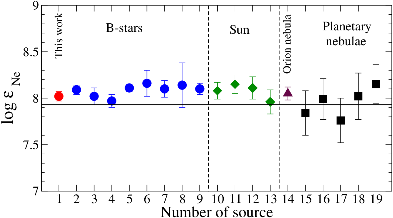
We compiled several neon abundance results recently obtained for B-stars, the Sun and the planetary nebulae (PNe) in the solar vicinity (Figure 9).
Our mean neon abundance from B-stars, log = 8.020.05, is in a good agreement with the solar photospheric neon abundance (8.080.09), calculated from recently revised ratio of neon to oxygen (Ne/O = 0.240.05) in the transition region of the quiet Sun (Young 2018), where the oxygen abundance, log = 8.690.05 dex, from Asplund et al. 2009 was adopted. The average quiet Sun does not show any FIP effect (Young 2005a), so these measurements are the most representative for the Sun. On the other hand, these measurements depend on the adopted oxygen solar abundance. For comparison, we took Ne abundance, log = 8.110.12 dex, derived from UV spectrum of a solar flare (Landi et al. 2007) as the absolute abundance of Ne in the solar atmosphere. Our result is by 0.09 dex lower than that, although still consistent within the error bars. Figure 9 also presents the comparison with the solar neon abundance from solar wind observations, log = 7.960.13 dex, (Bochsler 2007), that is by 0.06 dex lower that our result.
The H ii regions are relatively young objects. The nearest Galactic H ii region is the Orion nebula. Its chemical composition has been traditionally considered as the standard reference for the ionized gas in the solar neighborhood. Esteban et al. 2004 derived abundance in the Orion nebula gas for a large number of ions of different elements, including neon. They noticed that the abundances obtained from recombination lines are larger than those derived from collisionally excited lines. For example, the difference can reach 0.3 dex for neon assuming the temperature fluctuations ( = 0.0320.014). We adopted the value of neon abundance in the Orion nebula gas 8.050.07 dex obtained from collisionally excited lines and assuming the temperature fluctuations ( = 0.0220.002), as recommended by Esteban et al. 2004. Their value is only by 0.03 dex higher than the neon abundance in our B-stars (Fig. 9).
Planetary nebulae (PNe) are expanding shells of the luminous gas expelled by dying stars of low and intermediate masses (LIMS). They stem from objects that have lifetimes up to Gyrs. The ionized gas surrounding the central star shows emission lines of highly ionized species from which the abundances can be derived. The neon abundance can be compared and related to the results from stellar abundance analysis, since neon (and oxygen) originates from primary nucleosynthesis in massive stars (10 M⊙), and is therefore nearly independent on the evolution of LIMS, the progenitor stars of PNe (Henry 1989; Henry et al. 2004). For comparison, we collected several studies, where the neon abundances were obtained in PNe. We would not say that the abundances from PNe are very accurate, because the differences between abundances from collisionally excited lines and optical recombination lines can be much higher in PNe compared to those of H ii regions. For example, according to Wang & Liu 2007, in four Galactic disc PNe (He 2-118, H 1-35, NGC 6567, and M 1-61) the mean neon abundance calculated from collisionally excited lines is 7.780.23, while it is 8.720.60 from optical recombination lines. Figure 9 presents neon abundances from different sources, including five studies focused on PNe. In those studies, where it was mentioned, we adopted neon abundances obtained from collisionally excited lines, e.g. Tsamis et al. 2003; Wang & Liu 2007. The mean value of log = 7.840.24 was calculated on the basis of neon abundances in six Galactic disc PNe Wang & Liu 2007. The mean value of the neon abundance log = 7.990.22 dex was calculated from six PNe (Hu 1-2, IC 418, NGC 40, NGC 2440, NGC 6543, NGC 7662) with Galactocentric distances from 7.9 kpc to 8.9 kpc from summary of Pottasch & Bernard-Salas 2006. The value of log = 7.760.24 dex was derived from 16 Galactic planetary nebulae located at the Galactocentric distances from 8.0 to 8.9 kpc in Stanghellini et al. 2006. The log = 8.020.25 dex was obtained from Marigo et al. 2003 from three PNe (NGC 6543, NGC 7027, NGC 7662) which are located at the distances no more than 1.0 kpc. We adopted the mean value log = 8.150.21 dex, which was calculated from 16 Galactic PNe from Tsamis et al. 2003.
Our neon abundance from B-stars is consistent within the error bars with the all above-mentioned measurements of neon in PNe. However, the scatter is quite large for neon abundance obtained from PNe.
IV Conclusions
We present a neon model atom based on improved atomic data, the NLTE analysis for Ne i and Ne ii lines in the models representing the atmospheres of B-stars, and the consecutive determination of neon abundances in a sample of twenty-four B-stars in the solar neighborhood. The motivation of this work is to contribute to the solution of the ’Solar Model Problem’. Of course, only solar indicators can ever be a probe for the solar photospheric neon abundance. However, the counting all the physical effects makes the determination of solar neon abundance directly from solar indicators complicated. We believe that the indirect indicators, for example, B-stars from solar neighborhood could provide some indirect constraints on solar neon abundance. We obtained the mean neon abundance from twenty-four B-stars in solar neighborhood is log = 8.020.05. According to this result and considering Galactochemical evolution and radial stellar migration, it seems unlikely that the solar neon abundance is 8.29 (Bahcall et al. 2005b) that would be required to diminish the ’Solar Model Problem’ in helioseismology.
The model atom for Ne i – Ne ii has been constructed by using the most up-to-date atomic data and the non-local thermodynamic equilibrium (NLTE) line formation analysis was performed in classical 1D atmospheric models of B-type stars with the code detail. The use of the experimental oscillator strengths recently measured by Piracha et al. (2015) leads to smaller line-by-line scatter for the most investigated stars.
Our modeling predicts strong deviations from LTE for all considered Ne i lines and negative abundance corrections in the atmospheres with 10 400 30 400 K. For example, for Ne i 6402 Å line in the atmosphere with the parameters 17 500 / 3.8, corresponding to Her, the difference between NLTE and LTE abundances, , can reach up to 1.1 dex. We find that the main feature of Ne i is the extremely small photoionization cross-sections of the 3s levels, that leads to appreciable overpopulation of these levels. In contrast, the deviations from LTE for the most Ne ii lines are small and do not exceed 0.11 dex in the absolute value.
We perform chemical abundance analyses of 24 well studied B-type stars in the solar vicinity in the temperature range 10 400 33 400 K, using the the most recent data of experimental transition probabilities taken from Piracha et al. 2015. Our study is based on high-resolution and high S/N ratio stellar spectra, where S/N ratio is higher than 1000 for some of them. The abundances of neon are determined from Ne i and Ne ii lines in the optical and near-IR with LTE and NLTE line formation scenarios. We find that, for each star, NLTE leads to smaller line-to-line scatter. For five stars with both Ne i and Ne ii lines observed, NLTE provides ionization balance within 0.05 dex, while the LTE abundance difference can be as large as 0.50 dex in absolute value (e.g. HR 2928).
We find that the Ne i lines are quite sensitive to electron-collisional data variations. The using of R-matrix electron impact excitation calculations leads to strengthening of all Ne i lines by about 0.15 dex compared to the case, where the approximation formula by van Regemorter 1962 is applied for allowed transitions and the effective collision strength = 1 for the forbidden ones.
Our result is in accordance with previous neon estimations in B-stars (Kilian 1994; Sigut 1999; Dworetsky & Budaj 2000; Hempel & Holweger 2003; Cunha et al. 2006; Morel & Butler 2008; Takeda et al. 2010; Nieva & Przybilla 2012). The mean neon abundance from B-stars is also in agreement with the solar photospheric neon abundance, log = 8.080.09, calculated from the transition region of the quiet Sun (Young 2018), given that the oxygen abundance, log = 8.690.05 dex (Asplund et al. 2009) is adopted.
.
References
- Alexeeva et al. (2016) Alexeeva, S. A., Ryabchikova, T. A., & Mashonkina, L. I. 2016, MNRAS, 462, 1123, doi: 10.1093/mnras/stw1635
- Asplund et al. (2005) Asplund, M., Grevesse, N., & Sauval, A. J. 2005, in Astronomical Society of the Pacific Conference Series, Vol. 336, Cosmic Abundances as Records of Stellar Evolution and Nucleosynthesis, ed. I. Barnes, Thomas G. & F. N. Bash, 25
- Asplund et al. (2009) Asplund, M., Grevesse, N., Sauval, A. J., & Scott, P. 2009, ARA&A, 47, 481, doi: 10.1146/annurev.astro.46.060407.145222
- Auer & Mihalas (1973) Auer, L. H., & Mihalas, D. 1973, ApJ, 184, 151, doi: 10.1086/152313
- Bahcall et al. (2005a) Bahcall, J. N., Basu, S., Pinsonneault, M., & Serenelli, A. M. 2005a, ApJ, 618, 1049, doi: 10.1086/426070
- Bahcall et al. (2005b) Bahcall, J. N., Basu, S., & Serenelli, A. M. 2005b, ApJ, 631, 1281, doi: 10.1086/431926
- Bailey & Landstreet (2013) Bailey, J. D., & Landstreet, J. D. 2013, A&A, 551, A30, doi: 10.1051/0004-6361/201220671
- Basu & Antia (2008) Basu, S., & Antia, H. M. 2008, Phys. Rep., 457, 217, doi: 10.1016/j.physrep.2007.12.002
- Bochsler (2000) Bochsler, P. 2000, Reviews of Geophysics, 38, 247, doi: 10.1029/1999RG000063
- Bochsler (2007) —. 2007, A&A, 471, 315, doi: 10.1051/0004-6361:20077772
- Bodmer & Bochsler (2000) Bodmer, R., & Bochsler, P. 2000, J. Geophys. Res., 105, 47, doi: 10.1029/1999JA900434
- Butler (2008) Butler, K. 2008, Astronomy and Geophysics, 49, 6.23, doi: 10.1111/j.1468-4004.2008.49623.x
- Butler & Giddings (1985) Butler, K., & Giddings, J. 1985, Newsletter on the analysis of astronomical spectra, No. 9, University of London
- Caffau et al. (2011) Caffau, E., Ludwig, H. G., Steffen, M., Freytag, B., & Bonifacio, P. 2011, Sol. Phys., 268, 255, doi: 10.1007/s11207-010-9541-4
- Castelli & Kurucz (2003) Castelli, F., & Kurucz, R. L. 2003, in IAU Symposium, Vol. 210, Modelling of Stellar Atmospheres. Uppsala, Sweden, 17-21 June, 2002. Published on behalf of the IAU by the Astronomical Society of the Pacific, ed. N. Piskunov, W. W. Weiss, & D. F. Gray, A20
- Cunha et al. (2006) Cunha, K., Hubeny, I., & Lanz, T. 2006, ApJ, 647, L143, doi: 10.1086/507301
- Cunto et al. (1993) Cunto, W., Mendoza, C., Ochsenbein, F., & Zeippen, C. J. 1993, Bulletin d’Information du Centre de Donnees Stellaires, 42, 39
- Delahaye & Pinsonneault (2006) Delahaye, F., & Pinsonneault, M. H. 2006, ApJ, 649, 529, doi: 10.1086/505260
- Doherty (1962) Doherty, L. R. 1962, PhD thesis, The University of Michigan.
- Donati et al. (2006a) Donati, J.-F., Catala, C., Landstreet, J. D., & Petit, P. 2006a, in Astronomical Society of the Pacific Conference Series, Vol. 358, Solar Polarization 4, ed. R. Casini & B. W. Lites, 362
- Donati et al. (2006b) Donati, J.-F., Howarth, I. D., Jardine, M. M., et al. 2006b, MNRAS, 370, 629, doi: 10.1111/j.1365-2966.2006.10558.x
- Drake (2011) Drake, J. J. 2011, ApJ, 743, 22, doi: 10.1088/0004-637X/743/1/22
- Drake & Testa (2005) Drake, J. J., & Testa, P. 2005, Nature, 436, 525, doi: 10.1038/nature03803
- Dworetsky & Budaj (2000) Dworetsky, M. M., & Budaj, J. 2000, MNRAS, 318, 1264, doi: 10.1046/j.1365-8711.2000.03929.x
- Esteban et al. (2004) Esteban, C., Peimbert, M., García Rojas, J., et al. 2004, MNRAS, 355, 229, doi: 10.1111/j.1365-2966.2004.08313.x
- Feldman & Widing (2003) Feldman, U., & Widing, K. G. 2003, Space Sci. Rev., 107, 665, doi: 10.1023/A:1026103726147
- Ferrario et al. (2009) Ferrario, L., Pringle, J. E., Tout, C. A., & Wickramasinghe, D. T. 2009, MNRAS, 400, L71, doi: 10.1111/j.1745-3933.2009.00765.x
- Fossati et al. (2009) Fossati, L., Ryabchikova, T., Bagnulo, S., et al. 2009, A&A, 503, 945, doi: 10.1051/0004-6361/200811561
- Froese Fischer & Tachiev (2004) Froese Fischer, C., & Tachiev, G. 2004, Atomic Data and Nuclear Data Tables, 87, 1, doi: 10.1016/j.adt.2004.02.001
- Fuhr & Wiese (1998) Fuhr, J. R., & Wiese, W. L. 1998, in CRC Handbook of Chemistry and Physics, 79th edn., ed. D. R. Lide (Boca Raton, FL: CRC Press)
- Gaia Collaboration et al. (2018) Gaia Collaboration, Brown, A. G. A., Vallenari, A., et al. 2018, A&A, 616, A1, doi: 10.1051/0004-6361/201833051
- Geiss et al. (1970) Geiss, J., Hirt, P., & Leutwyler, H. 1970, Sol. Phys., 12, 458, doi: 10.1007/BF00148028
- Gies & Lambert (1992) Gies, D. R., & Lambert, D. L. 1992, ApJ, 387, 673, doi: 10.1086/171116
- Gloeckler & Geiss (2007) Gloeckler, G., & Geiss, J. 2007, Space Sci. Rev., 130, 139, doi: 10.1007/s11214-007-9189-z
- Griffin et al. (2001) Griffin, D. C., Mitnik, D. M., & Badnell, N. R. 2001, Journal of Physics B: Atomic Molecular Physics, 34, 4401, doi: 10.1088/0953-4075/34/22/310
- Hempel & Holweger (2003) Hempel, M., & Holweger, H. 2003, A&A, 408, 1065, doi: 10.1051/0004-6361:20030889
- Henry (1989) Henry, R. B. C. 1989, MNRAS, 241, 453, doi: 10.1093/mnras/241.3.453
- Henry et al. (2004) Henry, R. B. C., Kwitter, K. B., & Balick, B. 2004, AJ, 127, 2284, doi: 10.1086/382242
- Hibbert et al. (1993) Hibbert, A., Biemont, E., Godefroid, M., & Vaeck, N. 1993, A&AS, 99, 179
- Hovestadt et al. (1973) Hovestadt, D., Vollmer, O., Gloeckler, G., & Fan, C. Y. 1973, Phys. Rev. Lett., 31, 650, doi: 10.1103/PhysRevLett.31.650
- Hubeny & Lanz (1995) Hubeny, I., & Lanz, T. 1995, ApJ, 439, 875, doi: 10.1086/175226
- Hummer et al. (1993) Hummer, D. G., Berrington, K. A., Eissner, W., et al. 1993, A&A, 279, 298
- Kilian (1994) Kilian, J. 1994, A&A, 282, 867
- Kochukhov (2018) Kochukhov, O. 2018, BinMag: Widget for comparing stellar observed with theoretical spectra, Astrophysics Source Code Library. http://ascl.net/1805.015
- Kramida et al. (2019) Kramida, A., Ralchenko, Yu., Reader, J., & NIST ASD Team. 2019, NIST Atomic Spectra Database (ver. 5.7), [Online]. Available: https://physics.nist.gov/asd [2019, October 8]. National Institute of Standards and Technology, Gaithersburg, MD.
- Kurucz & Bell (1995) Kurucz, R. L., & Bell, B. 1995, Atomic line list (Kurucz CD-ROM, Cambridge, MA: Smithsonian Astrophysical Observatory)
- Kurucz & Peytremann (1975) Kurucz, R. L., & Peytremann, E. 1975, SAO Special Report No. 362
- Landi et al. (2007) Landi, E., Feldman, U., & Doschek, G. A. 2007, ApJ, 659, 743, doi: 10.1086/512035
- Landi & Testa (2015) Landi, E., & Testa, P. 2015, ApJ, 800, 110, doi: 10.1088/0004-637X/800/2/110
- Lanz & Hubeny (2007) Lanz, T., & Hubeny, I. 2007, ApJS, 169, 83, doi: 10.1086/511270
- Luo et al. (1989) Luo, D., Pradhan, A. K., Saraph, H. E., Storey, P. J., & Yu, Y. 1989, Journal of Physics B: Atomic Molecular Physics, 22, 389, doi: 10.1088/0953-4075/22/3/006
- Marigo et al. (2003) Marigo, P., Bernard-Salas, J., Pottasch, S. R., Tielens, A. G. G. M., & Wesselius, P. R. 2003, A&A, 409, 619, doi: 10.1051/0004-6361:20030953
- Molenda-Zakowicz & Polubek (2005) Molenda-Zakowicz, J., & Polubek, G. 2005, Acta Astron., 55, 375
- Morel & Butler (2008) Morel, T., & Butler, K. 2008, A&A, 487, 307, doi: 10.1051/0004-6361:200809924
- Nieva & Przybilla (2012) Nieva, M.-F., & Przybilla, N. 2012, A&A, 539, A143, doi: 10.1051/0004-6361/201118158
- Nieva & Przybilla (2014) —. 2014, A&A, 566, A7, doi: 10.1051/0004-6361/201423373
- Nieva & Simón Díaz (2011) Nieva, M.-F., & Simón Díaz, S. 2011, A&A, 532, A2, doi: 10.1051/0004-6361/201116478
- Pecaut et al. (2012) Pecaut, M. J., Mamajek, E. E., & Bubar, E. J. 2012, ApJ, 746, 154, doi: 10.1088/0004-637X/746/2/154
- Piracha et al. (2015) Piracha, N. K., Delanis, D., Kaminsky, J., et al. 2015, Canadian Journal of Physics, 93, 80, doi: 10.1139/cjp-2014-0192
- Pottasch & Bernard-Salas (2006) Pottasch, S. R., & Bernard-Salas, J. 2006, A&A, 457, 189, doi: 10.1051/0004-6361:20065548
- Przybilla et al. (2008) Przybilla, N., Nieva, M. F., & Butler, K. 2008, ApJ, 688, L103, doi: 10.1086/595618
- Przybilla et al. (2011) Przybilla, N., Nieva, M.-F., & Butler, K. 2011, Journal of Physics: Conference Series, 328, 012015, doi: 10.1088/1742-6596/328/1/012015
- Robrade et al. (2008) Robrade, J., Schmitt, J. H. M. M., & Favata, F. 2008, A&A, 486, 995, doi: 10.1051/0004-6361:200809690
- Rosman & Taylor (1998) Rosman, K. J. R., & Taylor, P. D. P. 1998, Journal of Physical and Chemical Reference Data, 27, 1275, doi: 10.1063/1.556031
- Ryabchikova et al. (2015) Ryabchikova, T., Piskunov, N., Kurucz, R. L., et al. 2015, Phys. Scr, 90, 054005, doi: 10.1088/0031-8949/90/5/054005
- Ryabchikova et al. (2016) Ryabchikova, T., Piskunov, N., Pakhomov, Y., et al. 2016, MNRAS, 456, 1221, doi: 10.1093/mnras/stv2725
- Rybicki & Hummer (1991) Rybicki, G. B., & Hummer, D. G. 1991, A&A, 245, 171
- Schneider et al. (2019) Schneider, F. R. N., Ohlmann, S. T., Podsiadlowski, P., et al. 2019, Nature, 574, 211, doi: 10.1038/s41586-019-1621-5
- Seaton (1962) Seaton, M. J. 1962, in Atomic and Molecular Processes, Academic Press Inc., U.S., ed. D. R. Bates, 375
- Seaton (1998a) Seaton, M. J. 1998a, Journal of Physics B: Atomic Molecular Physics, 31, 5315, doi: 10.1088/0953-4075/31/24/013
- Seaton (1998b) —. 1998b, MNRAS, 300, L1, doi: 10.1046/j.1365-8711.1998.01996.x
- Shearer et al. (2014) Shearer, P., von Steiger, R., Raines, J. M., et al. 2014, ApJ, 789, 60, doi: 10.1088/0004-637X/789/1/60
- Shulyak et al. (2004) Shulyak, D., Tsymbal, V., Ryabchikova, T., Stütz, C., & Weiss, W. W. 2004, A&A, 428, 993, doi: 10.1051/0004-6361:20034169
- Sigut (1999) Sigut, T. A. A. 1999, ApJ, 519, 303, doi: 10.1086/307355
- Sitnova et al. (2016) Sitnova, T. M., Mashonkina, L. I., & Ryabchikova, T. A. 2016, MNRAS, 461, 1000, doi: 10.1093/mnras/stw1202
- Sitnova et al. (2018) —. 2018, MNRAS, 477, 3343, doi: 10.1093/mnras/sty810
- Smith & Dworetsky (1993) Smith, K. C., & Dworetsky, M. M. 1993, A&A, 274, 335
- Sobelman (1992) Sobelman, I. I. 1992, Atomic Spectra and Radiative Transitions (Springer Series on Atoms and Plasmas; 2nd edition 1992, corr. print. 1996. p. cm.), 356, doi: 10.1007/978-3-642-76907-8
- Stanghellini et al. (2006) Stanghellini, L., Guerrero, M. A., Cunha, K., Manchado, A., & Villaver, E. 2006, ApJ, 651, 898, doi: 10.1086/507840
- Stankov & Handler (2005) Stankov, A., & Handler, G. 2005, ApJS, 158, 193, doi: 10.1086/429408
- Takeda et al. (2010) Takeda, Y., Kambe, E., Sadakane, K., & Masada, S. 2010, PASJ, 62, 1239, doi: 10.1093/pasj/62.5.1239
- Taylor et al. (1985) Taylor, K. T., Clark, C. W., & Fon, W. C. 1985, Journal of Physics B: Atomic Molecular Physics, 18, 2967, doi: 10.1088/0022-3700/18/14/020
- Tsamis et al. (2003) Tsamis, Y. G., Barlow, M. J., Liu, X. W., Danziger, I. J., & Storey, P. J. 2003, MNRAS, 345, 186, doi: 10.1046/j.1365-8711.2003.06972.x
- Vagnozzi et al. (2017) Vagnozzi, S., Freese, K., & Zurbuchen, T. H. 2017, ApJ, 839, 55, doi: 10.3847/1538-4357/aa6931
- van Regemorter (1962) van Regemorter, H. 1962, ApJ, 136, 906, doi: 10.1086/147445
- Wang & Liu (2007) Wang, W., & Liu, X. W. 2007, MNRAS, 381, 669, doi: 10.1111/j.1365-2966.2007.12198.x
- Wiese et al. (1966) Wiese, W. L., Smith, M. W., & Glennon, B. M. 1966, Atomic transition probabilities. Vol.: Hydrogen through Neon. A critical data compilation, ed. Wiese, W. L., Smith, M. W., & Glennon, B. M. (US Government Printing Office)
- Witthoeft et al. (2007) Witthoeft, M. C., Whiteford, A. D., & Badnell, N. R. 2007, Journal of Physics B: Atomic Molecular Physics, 40, 2969, doi: 10.1088/0953-4075/40/15/001
- Young (2005a) Young, P. R. 2005a, A&A, 439, 361, doi: 10.1051/0004-6361:20052963
- Young (2005b) —. 2005b, A&A, 444, L45, doi: 10.1051/0004-6361:200500206
- Young (2018) —. 2018, ApJ, 855, 15, doi: 10.3847/1538-4357/aaab48
- Zatsarinny & Bartschat (2009) Zatsarinny, O., & Bartschat, K. 2009, Physica Scripta Volume T, 134, 014020, doi: 10.1088/0031-8949/2009/T134/014020
- Zatsarinny & Bartschat (2012a) —. 2012a, Phys. Rev. A, 86, 022717, doi: 10.1103/PhysRevA.86.022717
- Zatsarinny & Bartschat (2012b) —. 2012b, Phys. Rev. A, 85, 062710, doi: 10.1103/PhysRevA.85.062710
- Zeman & Bartschat (1997) Zeman, V., & Bartschat, K. 1997, Journal of Physics B: Atomic Molecular Physics, 30, 4609, doi: 10.1088/0953-4075/30/20/021