microPhantom: Playing microRTS
under uncertainty and chaos
Abstract
This competition paper presents microPhantom, a bot playing microRTS and participating in the 2020 microRTS AI competition. microPhantom is based on our previous bot POAdaptive which won the partially observable track of the 2018 and 2019 microRTS AI competitions. In this paper, we focus on decision-making under uncertainty, by tackling the Unit Production Problem with a method based on a combination of Constraint Programming and decision theory. We show that using our method to decide which units to train improves significantly the win rate against the second-best microRTS bot from the partially observable track. We also show that our method is resilient in chaotic environments, with a very small loss of efficiency only. To allow replicability and to facilitate further research, the source code of microPhantom is available, as well as the Constraint Programming toolkit it uses.
Index Terms:
RTS Games, Competition, Decision-making, Uncertainty, Constraint Programming, Resilience.I Introduction
Recently, the Game AI community has seen a strong increase in the number of available AI competitions and environments. Although competitions can be great tools to stimulate and accelerate the research in Game AI, they may also bring a major drawback: having scripted, hard-coded bots tailored to win a competition, rather than taking risks by creating new AI techniques and improving existing ones.
microRTS is a minimalist real-time strategy game developed to be a convenient environment to test and improve Game AI techniques, historically Monte Carlo Tree Search techniques to tackle the combinatorial multi-armed bandit problem [3]. Like more complex game environments such as StarCraft, microRTS contains an imperfect information environment with a fog of war masking enemy units and buildings. What microRTS offers besides is a non-deterministic environment and requires less engineering than StarCraft to make a bot. Thanks to partially observable and non-determinism tracks, microRTS AI competitions propose challenging environments that push participants to go beyond a simple but efficient scripted bot.
In this paper, we present microPhantom, our new microRTS bot based on POAdaptive. The later was our microRTS bot that participated in the 2018 and 2019 microRTS AI competitions. The decision-making methods used in POAdaptive has been described in our previous paper [1] published in CEC 2019 proceedings. Therefore, Section IV briefly introducing POAdaptive shows nothing new, except the competition results in Section IV-D.
Like POAdaptive, microPhantom focuses on a decision-making problem under uncertainty, the Unit Production Problem, implemented and solved in Constraint Programming within our GHOST toolkit11 1 Available at github.com/richoux/GHOST [8]. This is where the name microPhantom comes from. POAdaptive and microPhantom are developed in Java, like microRTS, but GHOST being a C++ toolkit, the decision-making problem is coded in C++ and the constraint solver executable is called within the Java code.
This paper is organized as follows: Section II gives a short presentation of microRTS and its AI competitions. Section III introduce our Unit Production Problem as well as Constraint Programming and the Rank Dependent Utility, necessary to understand how decision making works within our bots. In Section IV, we summarize a presentation of POAdaptive’s decision-making method from our previous paper [1], and Section V introduces microPhantom and what is new compared to POAdaptive. This section contains an analysis of experimental results to attest to the efficiency of our decision-making method in partially observable environments. Finally, the paper concludes with some perspectives.
II microRTS
In this section, we briefly present the game microRTS and its annual AI competition.
II-A The game
microRTS, or RTS, is an open-source, minimalist real-time strategy (RTS) game developed by Santiago Ontañón for research purposes [3].

microRTS provide to players and researchers the main mechanisms one can find in RTS games. The game is played on a map, here a discrete grid. Usually, a map contains several resource patches. Once collected, this resource allows players to make buildings and train units. In microRTS, there are two kinds of buildings: bases producing worker units and stocking resources, and barracks training military units. Four types of units are available: workers, and three military units: light, ranged, and heavy units. Workers are weak against all units but are the only ones able to gather resources and construct buildings. All units must be on an adjacent case of an enemy unit or building to attack it, except the ranged unit able to attack at distance. Units have different attributes such as unit costs, unit hit points, unit speed, the time required to move, train, harvest, etc.
A game is played between two players, in 1v1. The game is real-time, meaning that players are doing their moves simultaneously, rather than turn by turn as in most strategy games. To win, a player must destroy all enemy units and buildings. If no player reaches that goal before a fixed number of game ticks, the game ends in a draw.
microRTS supports complete and partially observable games, i.e., without or with a fog of war, respectively, hiding enemy units and building if they are not within the sight range of our units and buildings. microRTS also supports deterministic and non-deterministic games, i.e., where unit damages are either deterministic or randomly drawn within a fixed range. This paper focuses on partially observable deterministic games.
II-B The competitions
The first microRTS competition has been organized in 2017 and was hosted by the IEEE Computational Intelligence in Games (CIG) 2017 conference [4]. Since 2017, an annual microRTS competition is organized at CIG, and now at CoG since the conference changed its name in 2019.
The three competitions from 2017 till 2019 were divided into 3 tracks: the standard track (complete information deterministic games), the non-deterministic track (complete information non-deterministic games), and the partially observable track (partially observable deterministic games).
Our bot POAdaptive participated in the 2018 and 2019 competition in the partially observable track (also in the standard track in 2018, even if the bot was designed to deal with the fog of war). Results of our bots in the partially observable track are given in Section IV-D.
The 2020 competition will be hosted by CoG 2020 and will be composed of 2 tracks only: the classic track (previously named standard track) and the partial observability track. All games are thus deterministic. Our new bot microPhantom will compete in the partial observability track; POAdaptive being removed from competitions.
In each track of each competition, two different rankings of bots are published: the ranking with open maps, i.e., maps that were officially listed in the rules of the competition, and the ranking of games played on both open and hidden maps, i.e., unknown maps from competitors.
III Decision-making under uncertainty
RTS games are excellent environments to develop and improve decision-making methods under uncertainty. Indeed, such games are rich enough to contain both challenging short-term and long-term decision-making problems. Besides, the fog of war implies partial observability of the game state, so players must take both tactical and strategic decisions under uncertainty.
microPhantom is part of a research project aiming to solve combinatorial optimization problems under uncertainty. Many decision-making problems can be expressed as combinatorial optimization problems, as soon as one aims to optimize one value while respecting some rules or impossibilities, giving a combinatorial flavor to the tackled problem. Thus, in particular, many RTS-related decision-making problems can be expressed as combinatorial optimization problems [8].
With microPhantom, we focus on the Unit Production Problem introduced below.
III-A The Unit Production Problem
As is usually the case in RTS games, units of microRTS follow a rock-paper-scissors pattern. Simulations introduced in our previous paper on the topic show that heavy units are efficient against light units, which are efficient against ranged units, which are in their turn efficient against heavy units [1].
The question captured by the Unit Production Problem is simple: without perfect information of the game state, in particular about the enemy army composition, and knowing my army composition, what units should I produce to counter the enemy army?
This decision-making problem under uncertainty can be modeled as a combinatorial optimization problem: we need to decide what units should we produce next, such that these units integrated into our current army offer the best counter to the partially-known enemy army while verifying some constraints such as not producing more units than our resource stock allows.
There exist different paradigms to model combinatorial optimization problems. In this paper, we model the Unit Production Problem in Constraint Programming.
III-B Constraint Programming
The basic idea behind Constraint Programming (CP) is to deal with combinatorial problems by splitting them up into two distinct parts: the first part is modeling your problem via one Constraint Programming formalism. This is usually done by a human being and this task must be ideally easy and intuitive. The second part consists in finding one or several solutions based on your model. This is done by a solver, i.e., a program running without any human interventions. Ideally, all the intelligence must be placed in this second part, and this is the main reason why CP is part of Artificial Intelligence.
Constraint Programming proposes many formalisms to model problems; the two most well-known are Constraint Satisfaction Problems (CSP) and Constrained Optimization Problems (COP). The former is to model decision problems, i.e., problems where the answer is either yes or no; the latter to model optimization problems, where we aim to maximize or minimize a value computed by an objective function.
Moreover, several formalisms dealing with uncertainty exist in CP: Mixed CSP, Probabilistic CSP, Stochastic CSP [10], etc. We recommend surveys [9, 2] on this topic to get familiar with these formalisms.
Unfortunately, no truly convenient formalism has been proposed in CP to model a decision-making problem where constraints are known and crisp but where the value to optimize depends upon some stochastic variables. In other words, our choices and possibilities are known, but a third-party agent we can only partially observe, such as a game environment with imperfect information, has a significant impact on the quality of our decisions.
In our previous paper [1], we presented a trick to model such decision-making problems under uncertainty with the regular COP formalism, and exploiting results from decision theory to handle uncertainty in the objective function. One of the main advantages of this trick is that one can use a regular CP solver since the problem has been modeled within a regular formalism. No need to develop a specific, ad-hoc solver able to handle uncertainty.
In this paper, we propose a different CP model to correct some issues in our previous model. Moreover, we model the Unit Production Problem where constraints are replaced by error functions. This allows us to make very powerful models: where CSP or COP models offer a network of constraints, i.e., a network of predicates expressing if variable assignments satisfy or not each constraint, our model contains a network of error functions expressing if variable assignments satisfy the constraints or, if not, how close they are to satisfy them. This allows expressing a finer structure about the problem: the error functions network is an ordered structure over invalid assignments a solver can exploit efficiently to improve the search. The major drawback is that such models are harder to define because it is not always obvious to find good error functions.
We consider error function networks as defined by Richoux and Baffier [7]. Formally, our error function network is defined by a tuple (, , ) such that:
- •
is a set of variables,
- •
is a domain, i.e., a set of values for variables in ,
- •
is a set of error functions with different scopes .
Error functions in are functions with being the arity of . An assignment , i.e., a tuple of values (one value in for each of the variables in the scope of ), is valid if and only if holds. All other strictly positive outputs of lead to invalid assignments. These positive outputs of are then interpreted like preferences over invalid assignments: the closer is to 0, the closer is to be a valid assignment for .
Before introducing our CP model used in microPhantom and comparing it with the one used in our previous bot POAdaptive, we give a short introduction on Rank Dependent Utility, the result from decision theory allowing us to handle uncertainty.
III-C Rank Dependent Utility
Since decision theory is already described in our previous paper [1], we will go straight to the point in this section by explaining what Rank Dependent Utility (RDU) is and how we use it in our CP models.
Rank Dependent Utility has been introduced by Quiggin [5, 6]. Like other notions in decision theory such as Expected Utility, RDU aims to define a preference for decisions by associating a probability to each possible consequence of each possible decision. But unlike Expected Utility, it allows modeling attraction or repulsion to risks through a probability deformation function. This can help to modify on-the-fly the behavior of an agent making a decision regarding its environment.
Let be a vector of consequences of an action and their associated outcome probability, such that with a consequence and the probability that the decision leads to consequence . The Rank Dependent Utility is then the function defined by Equation 1.
| (1) |
In Equation 1, is a utility function over the consequence space, intuitively giving a score to consequences, and an increasing function from to and interpreted as a probability deformation function. The function can be anything, as soon as it is monotone and both equalities and hold. Consequences in are ordered such that with , we have .
The intuition behind Equation 1 is the following: with probability , by making the given decision, you are sure to have at least the score of the worst consequence , i.e., . Then, with (deformed) probability , you can have the score plus the gain equals to . With probability , you can have an additional gain equals to , and so on until having an additional gain equals to with probability . The obtained value depends on the order, or rank, of the value of the utility function applied to consequences, justifying the name “Rank Dependent Utility”.

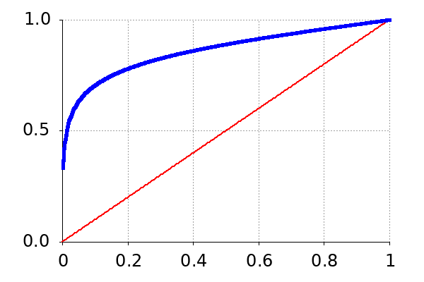

The probability deformation function allows to model risk-aversion where a concave function defines an attraction to risks and a convex function a repulsion to risks. Intuitively, if we have for all , then the agent taking a decision will underestimate gains probabilities and then will show a kind of pessimism about risks. We will have the opposite behavior if we have for all . Instead of a convex function, a sigmoid function can be used to model pessimism since it decreases the probabilities of good outcomes and increases the probabilities of unfavorable ones. Figure 2 illustrates the identity, a logit function, and a (shifted) logistic function we use in our bots to express neutrality, optimism, and pessimism, respectively.
We have now everything we need to present and compare CP models used in POAdaptive and microPhantom.
IV POAdaptive: 2018 - 2019
POAdaptive is the name of the bot playing to microRTS from which microPhantom is based. Its source code (CoG 2019 version) is available on our GitHub repository22 2 github.com/richoux/microrts-uncertainty/releases/tag/cog2019. Its main principles have been detailed in our CEC 2019 paper [1] but we recall here its CP model and how probability distributions have been handled.
IV-A CP model
The COP model for the Unit Production Problem implemented in POAdaptive is fairly simple, however we will only give here its intuitive description. The reader interested in the formal model is invited to find it in [1].
We need to describe what are our decision variables (the variable we can modify the value), the stochastic variables (handled by the environment, can only be partially observed), domains of all variables, our constraints, and our objective function to optimize.
Our model contains two kinds of decision variables: 1. variables to decide the number of light, ranged, and heavy units to produce, and 2. variables to decide how many units of type must be ideally assigned to fight against units of type . Our stochastic variables represent the number of light, ranged, and heavy units composing the enemy army.
Domains are the same for all variables: we consider each unit type in the game to be between 0 and 20 units, which is a fair assumption in microRTS.
Constraints are crisps, meaning there is no uncertainty within. Therefore, only decision variables appear in these constraints. We only have two types of constraints: 1. check if the number of units we aim to produce to not exceed our stock of resource, and 2. a constraint linking variables and such that holds for each type . In other words, the number of units of type we assigned to fight enemy units must be equals to the number of we plan to produce plus the number of we already have.
Finally, the objective function is to maximize such that
where is a constant in indicating how many units of type are required to beat one unit of type . These constants have been determined by running 200 skirmishes of 10 units against 10 units of all possible combinations. The minimum between 1 and the second part is here to forbid overkill, i.e., heavily defeating one type of enemy unit at the expense of other types.
IV-B RDU
Algorithm 1 from [1] describes how to compute the RDU value from the objective function of our CP model. The principle is simple: sample values of stochastic values in the scope of according to their probability distribution (Line 3). Then use as a utility function to give a score to the decision, i.e., the current assignment of the decision variables (Line 4). Repeat the operation times, sort the outputs of , and compute the RDU value according to Equation 1 (Line 7).
The pessimistic function we use is the shifted logistic function where is the probability and with parameters and . The optimistic function is the logit function with . These functions are depicted in Figure 2.
Observe that we consider a uniform distribution among possible inputs of the objective function , i.e., a probability is associated to each of the sampled inputs. We can do this since the real stochastic variables’ probability distribution is taken into account when we draw values of these stochastic variables following their probability distribution.
These distributions are made from the analysis of 800 replays of microRTS games from the 2017 competition. For each game tick and each unit type, we counted unit occurrence. These statistics are sharpened by observations while playing a game: if we observe for instance 3 enemy light units at the same moment, we nullify probabilities that the enemy has 0, 1 or 2 light units only, and we normalize the remaining probabilities.
IV-C Experimental results
To evaluate our decision-making process, we run games between the second-best bot of the competition, POLightRush bot, and four methods: POAdaptive using RDU with a pessimistic function, RDU with an optimistic function, RDU with as the identity function, and finally a baseline bot having the same behavior as POAdaptive except for the unit production decision, taken randomly among the three military units.
We run 100 games on each of 6 basic maps of different sizes, from to grids: 50 games where our bot started at the North-East position, and 50 at the South-West position. Then, we compute the normalized score like in microRTS competitions: we sum scores for each game, where the winner has a score of 1, the loser has 0, and both bots have 0.5 for draw games, then we divide total scores by the number of games played.
| Baseline | Neutral | Optimistic | Pessimistic |
| 40.00 | 42.93 | 44.93 | 44.5 |
Table I compiles 2.400 games in total and shows averages of normalized scores for the baseline bot and POAdaptive using a neutral, optimistic, and pessimistic function. We can see that POAdaptive with an optimistic or pessimistic function is doing slightly better than the baseline or POAdaptive with a neutral probability deformation function.
IV-D Competition results
POAdaptive participated in the partially observable track of the 2018 and 2019 microRTS AI competitions. Seven participants registered to the 2018 edition, and six to the 2019 edition. In both competitions, four baseline AIs were among the participants.


POAdaptive won both the 2018 and 2019 partially observable track, both on open maps only and on all maps. Figure 3 gives the final normalized scores on all maps. One can see that the POLightRush baseline bot was each time the most challenging opponent, this is why experiments in Sections IV-C and V-B take POLightRush as an opponent.
V microPhantom: 2020
microPhantom is the new name of POAdaptive, from which we improve the CP model, some parts of the code to be robust to rule modifications, and we changed the way to make the probability distribution of stochastic variables. The source code, as well as all experimental setups and results, are available on our GitHub repository33 3 github.com/richoux/microPhantom/tree/develop.
V-A Main differences with POAdaptive
V-A1 CP model
As written in Section III-B, we propose this time an error function-based model rather than a COP model.
We keep the same decision and stochastic variables and domains as described in Section IV-A. We defined error functions corresponding to the two types of constraint in the COP model, and add a third type of error function to express the idea that we cannot train more units than idle barracks we have. Our three kinds of error function are then:
We also changed the objective function to penalize the fact that a guessed number of enemy units of a given type is not beaten by the current assignment. We do this using the following function:
| (2) |

Our objective function becomes maximize with defined in Section IV-A. Injecting this regulation in our objective function gives it a new interpretation while using an optimistic or pessimistic probability deformation function: with an optimistic function, we will favor assignments that fit the best what we think in average what the enemy composition is, so we maximize our composition to be the best counter. With a pessimistic function, we will consider more worst cases for us, i.e., that the opponent is making a good counter against our army, so we maximize resilience here, to be prepared for the worst. In other words, we try to minimize bad surprises.
V-A2 Stochastic variables estimation
For POAdaptive, we made the probability distributions of our stochastic variables by analyzing replays, and we draw the value of each stochastic variable following its distribution and the number of game ticks. The issue with that method is that replays we analyzed won’t certainly fit the strategy of our current opponent.
To get around this problem, we now start each game with a uniform distribution for a unique random variable representing the chance to draw one light, heavy, or ranged unit from the enemy army. This distribution is updated such that probability for each value (i.e., for each type of units ), we have
where is the number of enemy units of type we observe at the moment, the number of enemy units of type we observed since the beginning of the game, minus destroyed units and units in , and total is the sum of numerators of , , and to have . Enemy units we currently observe count twice compared to units we saw in the past to be more reactive if the opponent switches his or her strategy, and we add on the numerator to never have a probability to produce any unit type.
Then, we estimate the resource the opponent gathered since the beginning of the game, regarding his or her number of workers, the harvesting time, worker’s speed, how many resources a worker can carry, and the average distance of resource patches to the enemy base, considering it has a similar placement as our. We subtract to this estimation the sum of the cost of enemy units we destroyed and the sum of the cost of enemy units we observed, as well as the cost of a base and a barracks if building them was required. What remains is an estimation of the resource we do not know how it has been spent by the opponent.
Now, we only draw a value of our unique random variable to know what is the type of an enemy unit we probably do not see yet. We subtract its cost to the estimated remaining enemy resource stock and we continue until not enough resource left. We add these estimated values to the number of enemy units currently observed for each unit type, and we have our estimation of the enemy army composition. We repeat these draws each time we need to estimate the enemy army composition.
This way, we have a sharper estimation of the enemy army composition which is adapted to the specific opponent we are currently playing against.
V-A3 Chaotic-robust decision-making
microPhantom’s code contains as few hard-coded game values as possible. Thus, any attributes of the game can change (cost of units and buildings, time to train/move/harvest, hit points, etc) event during the game, and the decision-making process will not be perturbed. We call chaotic environments such environments where attributes are deterministic but change from game to game.
V-A4 In-game function replacement
POAdaptive used an optimistic or pessimistic probability deformation function regarding the map size, and stick with the same function during the whole game.
microPhantom can switch from the three functions defined in Section IV-B regarding its current situation. It starts with a neutral function and will switch to the optimistic function if the sum of the cost of destroyed enemy units is greater than the cost of its destroyed units, added to twice the cost of the cheapest unit. On the other way around, it switches to the pessimistic function.
V-A5 Domain knowledge-based actions
microPhantom contains some hard-coded, domain knowledge-based actions POAdaptive did not have, such as producing more workers if several resource patches are near our base, and building more barracks if it is gathering resources faster than it can spend them.
V-B Experimental results
Some domain knowledge-based actions we added to microPhantom improve the bot significantly. To measure improvements due to our non-scripted modifications, namely the new CP model, the new stochastic variables sampling and the in-game function replacement, we run the same experiments than in Section IV-C on 6 basic maps, with two additions: we also consider the 8 open maps from microRTS AI competitions, and we also run experiments within a chaotic environment to test microPhantom’s decision-making robustness.
The baseline bot has again the same code than microPhantom except for the unit production behavior. There is one domain knowledge-based action coded into the unit production behavior, forcing microPhantom to produce twice the fastest unit to produce at the beginning of a game on a small map (with a surface smaller than 144, i.e., a grid map). This domain knowledge-based action has been disabled during experiments to have a fair comparison of microPhantom and its baseline on small maps.
microPhantom asks the constraint solver to decide about what units should be produced at each frame where at least one barracks is ready for training. Solving the Unit Production Problem is done within 100ms, whatever the situation: map size, army composition, etc.
Finally, all maps have been played 100 times by each bot, versus the POLightRush bot. Our bots played 50 times at the Player 1 starting position (North-West on basic maps, but it can be elsewhere on open maps) and 50 times at the Player 2 starting position (South-East on basic maps), on each map. In chaotic environments, our bots played once at the Player 1 and the Player 2 position with the same configuration setting, i.e., the same attributes of the game. Then, this configuration setting is randomized before each new couple of games.
| Bots | Basic maps | Open maps |
|---|---|---|
| Baseline | 61.75 | 64.87 |
| microPhantom | 73.25 | 76.00 |
| microPhantom chaos | 70.91 | 67.93 |
Table II compiles 4,200 games in total: 1,800 on basic maps and 2,400 on open maps. It shows averages of normalized scores for microPhantom, both in fixed and chaotic environments, and its baseline in a fixed environment. Notice that the version of POLightRush used for games in Table II is an enhanced version compare to the one used for games in Table I.
We can see that, despite playing against a stronger POLightRush bot, results of the baseline based on microPhantom in Table II are greatly better than results from the baseline based on POAdaptive in Table I. This difference is due to domain knowledge-based actions we added in microPhantom. We are then able to quantify improvements due to these hard-coded modifications: they lead to an increase of approximately 50% of the win rate against POLightRush bot. A finer analysis of result data tells us that this gain comes mostly from the conversion of draw games into won games.
Table II shows a significant improvement of microPhantom compare to its baseline, clearly more significant than POAdaptive results in Table I. This is only due to our improved unit production behavior compare to POAdaptive.
microPhantom’s results on chaotic environments are similar to fixed ones, showing that microPhantom is perfectly able to handle rule changes without disturbing its decision-making process. The score on open maps seems significantly different though, with a score of 67.93 in chaotic environments against 76 in fixed ones. Actually, this is only due to one open map, NoWhereToRun, which is very small () where the two players are separated by a thin wall of resources. Usually, microPhantom nearly always win against POLightRush bot on this map, but in chaotic environments, workers have one chance over two to be able to carry 2 resources instead of 1. In that configuration, a hole is very quickly made in the wall and let enter light units from the POLightRush bot. A close look at the results data show us that microPhantom is nearly winning 50% of the time against POLightRush bot on this map in a chaotic environment (45 wins, 7 ties and 48 losses). Actually, microPhantom wins when workers can only carry one resource at the time, letting it more time to prepare its defenses, and loses when workers can carry 2 resources. Without this very specific situation, microPhantom’s score would be similar in both fixed and chaotic environments: if we consider the same score than the fixed one on NoWhereToRun, the score of microPhantom in chaotic environments on open maps turns to be 74.
microPhantom is also theoretically able to handle rule changes in a middle of a game (a truly chaotic environment), but this seems not easy to process with the current version of microRTS.
VI Conclusion and perspectives
In this paper, we present our bot microPhantom playing microRTS. We show its main differences and improvements compare to its predecessor POAdaptive, winner of the partially observable track of the 2018 and 2019 microRTS AI competition, and show through an experimental evaluation including 4.200 games that we achieve significant improvements thanks to better decision-making under uncertainty.
We also make microPhantom able to handle rule changes: the decision-making mechanism in the bot is resilient to the modification of many game attributes.
Unfortunately, the 2020 edition of the microRTS AI competition does not propose a non-deterministic track anymore, unlike previous editions. This track run games where each attack makes damage between a range fixed for each unit type. We think such a track has its place in the AI competition since it limits hard-coded, scripted bots tailored for the competition and force them to develop and implement AI techniques to get around non-determinism, but we guess it has been removed due to a lack of participants. We propose that next microRTS AI competition should contain an even bolder chaotic track where many if not all game attributes change at each game, or even during a game.
We may improve microPhantom’s CP model by defining better error functions. This could be done for instance by using the automatic method proposed by Richoux and Baffier [7] to find good error functions.
Finally, microRTS is certainly too minimalist to contains many challenging combinatorial optimization problems, with or without uncertainty. We plan to develop a StarCraft bot using massively the decision-making method presented in this paper to tackle different aspects of the game, from economic development and strategy decisions to micro-management.
References
- [1] V. Antuori and F. Richoux, “Constrained optimization under uncertainty for decision-making problems: Application to Real-Time Strategy games,” in Proceeding of the Congress on Evolutionary Computation (CEC). IEEE, 2019, pp. 450–457.
- [2] B. Hnich, R. Rossi, S. A. Tarim, and S. Prestwich, A Survey on CP-AI-OR Hybrids for Decision Making Under Uncertainty. Springer New York, 2011, pp. 227–270.
- [3] S. Ontañón, “The Combinatorial Multi-armed Bandit Problem and Its Application to Real-time Strategy Games,” in Proceedings of the 9th AAAI Conference on Artificial Intelligence and Interactive Digital Entertainment (AIIDE’13), 2014, pp. 58–64.
- [4] S. Ontañón, N. A. Barriga, C. R. Silva, R. O. Moraes, and L. H. S. Lelis, “The first microrts artificial intelligence competition,” AI Magazine, vol. 39, no. 1, pp. 75–83, 2018.
- [5] J. Quiggin, “A Theory of Anticipated Utility,” Journal of Economic Behavior & Organization, vol. 3, pp. 323–343, 1982.
- [6] ——, Generalized Expected Utility Theory: The Rank Dependent Model. Springer, 1993.
- [7] F. Richoux and J.-F. Baffier, “Automatic Cost Function Learning with Interpretable Compositional Networks,” arXiv, 2020.
- [8] F. Richoux, A. Uriarte, and J.-F. Baffier, “GHOST: A Combinatorial Optimization Framework for Real-Time Problems,” IEEE Transactions on Computational Intelligence and AI in Games, vol. 8, no. 4, pp. 377–388, 2016.
- [9] G. Verfaillie and N. Jussien, “Constraint solving in uncertain and dynamic environments: A survey,” Constraints, vol. 10, no. 3, pp. 253–281, 2005.
- [10] T. Walsh, “Stochastic Constraint Programming,” in Proceedings of the 15th Eureopean Conference on Artificial Intelligence (ECAI’02), 2002, pp. 111–115.