Janus interface entropy and Calabi’s diastasis in four-dimensional $\mathcal{N}=2$ superconformal field theoriesPreprint: RIKEN-iTHEMS-Report-20, UT-Komaba-20-1

We begin by reviewing the standard definition of the entanglement entropy, with a conformal interface included in a straightforward way. For a similar discussion with defects of general codimensions, see Kobayashi:2018lil.

We consider a 4$d$ CFT in Minkowski space with coordinates $(t,y^{1},y^{2},y^{3})$. Let us introduce along the hyperplane $y^{3}=0$ a conformal interface ${\cal I}$ that preserves a subgroup $SO(2,3)$ of the conformal group $SO(2,4)$. We also use spherical coordinates $(r,\phi,\chi)$ related to the Cartesian coordinates as $(y^{1},y^{2},y^{3})=(r\sin\phi\cos\chi,r\sin\phi\sin\chi,r\cos\phi)$. Let us take the entangling surface $\Sigma$ to be a 2-sphere with radius $R$ inside the $t=0$ time slice

$\displaystyle\Sigma=\{t=0,\,r=R\}\ .$

(9)

We decompose the Hilbert space modified by ${\mathcal{I}}$, $\mathcal{H}_{\mathcal{I}}$, into the tensor product of $\mathcal{H}_{A}$ and $\mathcal{H}_{B}$ that correspond to the regions $r<R$ and $r>R$ in the constant time slice $\mathbb{R}^{3}$ at $t=0$, respectively:¹¹ 1 We choose not to delve into to the subtleties associated with such a decomposition for a gauge theory.

$$\mathcal{H}_{\mathcal{I}}=\mathcal{H}_{A}\otimes\mathcal{H}_{B}\,.$$

(10)

Inside the $t=0$ slice, the entangling surface $r=R$ intersects the interface along the great circle at $\phi=\pi/2$. Using the ground state $|0\rangle\in\mathcal{H}_{\mathcal{I}}$ we form the density matrix $\rho={\rm tr}_{B}|0\rangle\langle 0|$ by the partial trace over $\mathcal{H}_{B}$. Next, by taking the partial trace over $\mathcal{H}_{A}$ we define the entanglement entropy

$$S_{E}^{\text{(ICFT)}}:=-{\rm tr}_{A}\,\rho\log\rho\ ,$$

(11)

and the Rény entropy

$$S_{n}^{\text{(ICFT)}}:=\frac{1}{1-n}\log{\rm tr}_{A}\,\rho^{n}\,.$$

(12)

The two quantities are related as

$$\lim_{n\rightarrow 1}S_{n}^{\text{(ICFT)}}=S_{E}^{\text{(ICFT)}}\ .$$

(13)

By construction $S_{E}^{\text{(ICFT)}}$ and $S_{n}^{\text{(ICFT)}}$ are non-negative.

The replica trick identifies the quantity ${\rm tr}_{A}\,\rho^{n}$ with the partition function $Z[{\cal M}_{n}]$, i.e., the path integral on the $n$-fold branched cover $\mathcal{M}_{n}$ of the Euclidean space $\mathbb{R}^{4}$, normalized by $Z[{\cal M}_{1}]^{n}$:

$${\rm tr}_{A}\,\rho^{n}=\frac{Z[{\cal M}_{n}]}{Z[{\cal M}_{1}]^{n}}\ .$$

(14)

Since we are interested in the continuous limit $n\rightarrow 1$, we wish to define $\mathcal{M}_{n}$ for non-integer $n$.

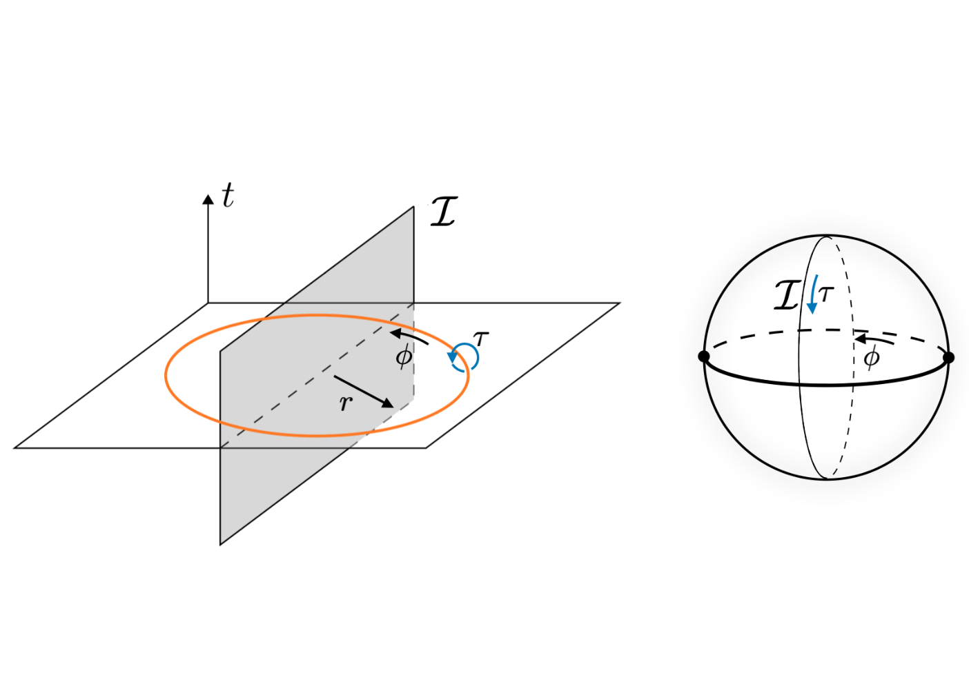
A useful tool to achieve this is the so-called Casini–Huerta–Myers map Casini:2011kv; Jensen:2013lxa. We perform the Wick rotation via the substitution $t\rightarrow-{\rm i}t$ and consider the Euclidean space with coordinates $(t,y^{1},y^{2},y^{3})$ and the metric

$\displaystyle\begin{aligned} \mathrm{d}s_{\mathbb{R}^{4}}^{2}&=\mathrm{d}t^{2}+\mathrm{d}r^{2}+r^{2}\,\left(\mathrm{d}\phi^{2}+\sin^{2}\phi\,\mathrm{d}\chi^{2}\right)\ .\end{aligned}$

(15)

Let us perform a change of coordinates to $(\tau,\theta,\phi,\chi)$ via (the Euclidean version of) the Casini--Huerta--Myers (CHM) map²² 2 We believe that the reader can distinguish, based the context, the coordinate $\tau$ from the coupling $\tau$.

$\displaystyle\begin{aligned} t&=R\,\frac{\sin\theta\sin\tau}{1+\sin\theta\cos\tau}\ ,\\ r&=R\,\frac{\cos\theta}{1+\sin\theta\cos\tau}\ .\end{aligned}$

(16)

Through this, the Euclidean space is conformally equivalent to the round sphere as

$\displaystyle\mathrm{d}s_{\mathbb{R}^{4}}^{2}=\Omega^{2}\mathrm{d}s_{\mathbb{S}^{4}}^{2}\ ,$

(17)

with the conformal factor

$\displaystyle\Omega=\frac{R}{1+\sin\theta\cos\tau}$

(18)

and the round sphere metric

$\displaystyle\mathrm{d}s_{\mathbb{S}^{4}}^{2}=\mathrm{d}\theta^{2}+\sin^{2}\theta\,\mathrm{d}\tau^{2}+\cos^{2}\theta\,\left(\mathrm{d}\phi^{2}+\sin^{2}\phi\,\mathrm{d}\chi^{2}\right)\ .$

(19)

The entangling surface $\Sigma$ is mapped to the 2-sphere at $\theta=0$. The translation in the $\tau$ direction fixes $\Sigma$ and corresponds to the modular flow generated by the modular Hamiltonian $H$ defined by $\rho=e^{-H}$ Casini:2011kv. See Figure 1. The $n$-fold cover $\mathcal{M}_{n}$ has the metric

$$\mathrm{d}s_{\mathcal{M}_{n}}^{2}=\Omega^{2}\mathrm{d}s_{\mathbb{S}^{4}_{n}}^{2}\ ,$$

(20)

with

$\displaystyle\mathrm{d}s_{\mathbb{S}^{4}_{n}}^{2}$

$\displaystyle=\mathrm{d}\theta^{2}+n^{2}\sin^{2}\theta\,\mathrm{d}\tau^{2}+\cos^{2}\theta\,\left(\mathrm{d}\phi^{2}+\sin^{2}\phi\,\mathrm{d}\chi^{2}\right)\ .$

(21)

The range of $\tau$ is $0\leq\tau<2\pi$. This metric is singular for $n\neq 1$.

Armed with the CHM map (20) associating the replica space ${\cal M}_{n}$ to the $n$-fold cover of a 4-sphere $\mathbb{S}_{n}^{4}$, we will derive a relation between the entanglement entropy and the sphere partition function in ICFT. While we are only concerned with ICFT in four dimensions there is no difficulty in repeating the same argument for the CHM map in general $d$ dimensions (just by replacing the entangling region $\mathbb{S}^{2}$ with $\mathbb{S}^{d-2}$). So we closely follow the derivation in Kobayashi:2018lil which uses the dimensional regularization for calculating the entanglement entropy in CFT with conformal defects for a moment. This approach is not only general enough, but also simplifies the derivation by avoiding an extra care for conformal anomalies as they are automatically incorporated into poles at even dimensions. We defer the discussion about conformal anomalies in ICFT to Section 6.4.

In the dimensional regularization we adopt a scheme such that the theory is strictly conformal even at quantum level. In other words, we start with an odd-dimensional CFT without conformal anomalies and analytically continue it to general dimensions. Hence the CFT partition functions, even in the presence of an interface, on the $n$-fold covers of the Euclidean space and $d$-sphere are the same under conformal transformation of the type (20):

$\displaystyle Z^{\text{(ICFT)}}[{\cal M}_{n}]=Z^{\text{(ICFT)}}[\mathbb{S}^{d}_{n}]\ .$

(22)

Note that the equality between the two partition functions holds only up to power-law UV divergences. It follows from this relation together with (12) and (14) that the Rényi entropy across a sphere in ICFT is given by

$\displaystyle S_{n}^{\text{(ICFT)}}=\frac{1}{1-n}\,\log\frac{Z^{\text{(ICFT)}}[\mathbb{S}^{d}_{n}]}{\left(Z^{\text{(ICFT)}}[\mathbb{S}^{d}]\right)^{n}}\ .$

(23)

We note that this expression is trivially valid in the absence of an interface.

Now we consider an interface CFT built out of two CFTs, CFT₊ and CFT_-, glued together along the interface ${\cal I}$. We define the interface entropy as the contribution to the entanglement entropy by the interface ${\cal I}$:

$\displaystyle S_{\cal I}\equiv S_{E}^{\text{(ICFT)}}-\frac{S_{E}^{\text{(CFT${}_{+}$)}}+S_{E}^{\text{(CFT${}_{-}$)}}}{2}\ .$

(24)

Using (13) and (23) we can write the quantity $S_{E}^{\text{(ICFT)}}$ in (24) as

$$S_{E}^{\text{(ICFT)}}=\log\,Z^{\text{(ICFT)}}[\mathbb{S}^{d}]-\left.\partial_{n}\log Z^{\text{(ICFT)}}[\mathbb{S}^{d}_{n}]\right|_{n=1}\,.$$

(25)

We wish to show that the second term in (25) vanishes, i.e., that the relation

$$S_{E}^{\text{(ICFT)}}=\log\,Z^{\text{(ICFT)}}[\mathbb{S}^{d}]$$

(26)

holds. For this we need the behavior of the Rényi entropy (23) in ICFT at $n=1+\epsilon$ with small $\epsilon$. In the framework of general, not necessarily supersymmetric, conformal field theory, $\log Z^{\text{(ICFT)}}[\mathbb{S}^{d}_{n}]$ and $\log Z^{\text{(ICFT)}}[\mathbb{S}^{d}]$ differ by the variation of the background metric $\delta g_{\tau\tau}=(n^{2}-1)\,\sin^{2}\theta$. In terms of the stress tensor defined by

$\displaystyle\langle T^{\mu\nu}\rangle=-\frac{2}{\sqrt{g}}\,\frac{\delta\,\log Z}{\delta g_{\mu\nu}}\ ,$

(27)

where $Z$ is a general partition function that depends on the metric, we can write

$$-\log\,Z^{\text{(ICFT)}}[\mathbb{S}^{d}_{n}]+\log\,Z^{\text{(ICFT)}}[\mathbb{S}^{d}]=+\frac{1}{2}\int_{\mathbb{S}^{d}}\,\delta g_{\mu\nu}\,\langle\,T^{\mu\nu}\,\rangle_{\mathbb{S}^{d}}^{\text{(ICFT)}}+{\cal O}(\epsilon^{2})\ .$$

(28)

To study the one-point function of the stress tensor we use a conformal mapping between $\mathbb{S}^{d}$ and the flat space. This map may be but does not have to be the CHM map (16). In general the one-point function $\langle\,T^{\mu\nu}\,\rangle_{\mathbb{S}^{d}}^{\text{(ICFT)}}$ transforms under a conformal transformation as

$\displaystyle\langle\,T_{\mu\nu}\,\rangle^{(\text{ICFT})}_{\mathbb{S}^{d}}=(\text{Weyl factor})^{2}\langle\,T_{\mu\nu}\,\rangle^{(\text{ICFT})}_{\mathbb{R}^{d}}\ .$

(29)

One can easily show $\langle\,T_{\mu\nu}\,\rangle^{(\text{ICFT})}_{\mathbb{R}^{d}}$ vanishes due to the residual conformal symmetry $SO(1,4)$ preserved by the interface McAvity:1995zd; Billo:2016cpy, so we conclude that the interface entropy is given by the combination

$\displaystyle S_{\cal{I}}=\log\left[\frac{Z^{\text{(ICFT)}}[\mathbb{S}^{d}]}{(Z^{\text{(CFT${}_{+}$)}}[\mathbb{S}^{d}]\,Z^{\text{(CFT${}_{-}$)}}[\mathbb{S}^{d}])^{1/2}}\right]\ ,$

(30)

of the sphere partition functions with and without an interface. In what follows we will use this relation in the calculation of the interface entropy in $d=4$ dimensions.

We now turn to half-BPS superconformal interfaces in 4$d$ $\mathcal{N}=2$ superconformal field theories. For our conventions, see Appendix A.1.

In flat space with Cartesian coordinates $y^{\mu}$ the Poincaré supersymmetry and special superconformal transformations are parametrized as $\delta_{Q}=\overline{\epsilon}{}^{i}Q_{i}+\overline{\epsilon}_{i}Q^{i}$ and $\delta_{S}=\overline{\eta}{}^{i}S_{i}+\overline{\eta}_{i}S^{i}$, where a bar on a 4-component spinor parameter indicates the Weyl conjugate defined in (163).³³ 3 The parameters here are related to the parameters in Appendix A.3 as $(\epsilon^{i},\epsilon_{i})_{\text{there}}=(\epsilon^{i}+y^{\mu}\gamma_{\mu}\eta^{i},\epsilon_{i}+y^{\mu}\gamma_{\mu}\eta_{i})$. The spinors $\epsilon^{i}$ and $\eta_{i}$ are left-handed, while $\epsilon_{i}$ and $\eta^{i}$ are right-handed. The operators $Q_{i}$ and $S^{i}$ are left-handed, while $Q^{i}$ and $S_{i}$ are right-handed. A half-BPS superconformal interface at $y^{3}=0$ preserves the fermionic symmetries with parameters satisfying

$$\epsilon_{i}=\rho_{ij}\gamma^{3}\epsilon^{j}\ ,\quad\eta_{i}=-\rho_{ij}\gamma^{3}\eta^{j}\ ,$$

(31)

where the fixed symmetric tensor $\rho_{ij}$ satisfies $\rho_{ij}\overline{\rho}^{jk}=\delta_{i}^{k}$ with $\overline{\rho}^{ij}:=(\rho_{ij})^{*}$.⁴⁴ 4 Such $\rho_{ij}$ can be parametrized as $\rho_{ij}=e^{{\rm i}\alpha}\vec{n}\cdot\vec{\tau}_{ij}$, where $\alpha$ is real and $\vec{n}$ is a real unit vector. They transform under $U(1)_{R}$ and $SU(2)_{R}$. In other words, the preserved supercharges and special superconformal charges are

$$Q_{i}-\rho_{ij}\gamma_{3}Q^{j}\ ,\quad S_{i}+\rho_{ij}\gamma_{3}S^{j}\,.$$

(32)

They generate the 3$d$ $\mathcal{N}=2$ superconformal algebra $OSp(2|4)_{sc}$.

Since such an interface is a special kind of conformal interface, our discussion in Sections 2.1 and 2.2 applies to it. There are, however, two important differences between the conformal case and the superconformal case.

The first difference is that superconformal field theories and interfaces naturally couple to background supergravity (or conformal supergravity) fields other than the metric. The partition functions are functionals of these fields. In general a supersymmetric background involves non-zero supergravity fields.⁵⁵ 5 In the supersymmetric $\mathbb{S}^{4}$ background, the metric is the only non-zero field in the Poincaré supergravity multiplet Hama:2012bg; Pestun:2014mja. There are non-zero fields in compensating multiplets Gomis:2014woa that violate conformal invariance and unitarity. See (95) and (96).

The second difference is that the counterterms dictated by supersymmetry involve supergravity fields other than the metric. When we turn off supergravity fields other than the metric, as in the supersymmetric $\mathbb{S}^{4}$ background, such terms reduce to non-SUSY counterterms that involve only the metric (and other non-supergravity background fields), but their coefficients are related by supersymmetry. This mechanism gives universal meanings to some, a priori non-universal, terms in the effective action Gerchkovitz:2014gta.

To establish the relation (4) between the interface entropy and Calabi’s diastasis, an important step for us—Step 3 in the introduction—involves localization that computes the supersymmetric partition function $Z^{\mathcal{I}}_{\text{SUSY}}[\mathbb{S}^{4}]$ of the system with an interface in a supersymmetric background. As we will see in Section 4, the SUSY partition function $Z^{\mathcal{I}}_{\text{SUSY}}[\mathbb{S}^{4}]$ is in general complex. On the other hand, so far we have related the interface entropy only to the conformal partition function $Z^{\text{(ICFT)}}[\mathbb{S}^{4}]$, which is real and positive by unitarity.

Based on these motivations we make the assumption (6) in Step 2, i.e.,

$$\quad Z^{\text{(ICFT)}}[\mathbb{S}^{4}]=\left|Z^{\mathcal{I}}_{\text{SUSY}}[\mathbb{S}^{4}]\right|.$$

(33)

Combined with (30), this gives the interface entropy

$\displaystyle S_{\cal{I}}=\log\left[\frac{\left|Z^{\mathcal{I}}_{\text{SUSY}}[\mathbb{S}^{4}]\right|}{(Z^{\text{(CFT${}_{+}$)}}_{\text{SUSY}}[\mathbb{S}^{4}]\,Z^{\text{(CFT${}_{-}$)}}_{\text{SUSY}}[\mathbb{S}^{4}])^{1/2}}\right]\ ,$

(34)

in terms of supersymmetric sphere partition functions with and without an interface. We note that the combination (34) coincides with the “boundary free energy” considered in Gaiotto:2014gha; DiPietro:2019hqe; Gupta:2019qlg.⁶⁶ 6 In 3$d$ it is common to define the free energy as $F=-\log|Z_{\text{SUSY}}[{\mathbb{S}^{3}}]|$ in terms of the absolute value of the partition function computed by SUSY localization. See for example Jafferis:2011zi.

We explain in Section 6.1 that one can use the super-Weyl anomaly of Bachas:2016bzn to prove the 2$d$ version of the assumption (33).

We now explain that the assumption (33) is natural from the point of view of the supersymmetric Rényi entropy Nishioka:2013haa. More precisely (33) is equivalent to the statement that the entanglement entropy $S_{E}^{\text{(ICFT)}}$ coincides with the $n\rightarrow 1$ limit of the supersymmetric Rényi entropy $S_{{\rm SUSY}\ n}^{\text{(ICFT)}}$ that we define below.

Even in the presence of a conformal interface, one can relate the (ordinary) Rényi entropy to the partition function on the $n$-fold covering of the round sphere, as we wrote in (23). This expression is somewhat formal because we do not specify how we deal with the conical singularities for $n\neq 1$. One can make it more precise by considering a supersymmetric background $\widetilde{\mathbb{S}}^{4}_{n}$ that regularizes the $n$-fold covering $\mathbb{S}^{4}_{n}$ Huang:2014pda; Pestun:2014mja. We review the supergravity background $\widetilde{\mathbb{S}}^{4}_{n}$ in Appendix C.1.⁷⁷ 7 Although we do not show this explicitly, we expect that in the supersymmetric $\widetilde{\mathbb{S}}^{4}_{n}$ background one can construct a SUSY preserving Janus interface that reduces to the half-BPS interface in the $n\rightarrow 1$ limit. The worldvolume of the interface is invariant under the Killing vector generated by the square of the supercharge preserved by the background. The $\widetilde{\mathbb{S}}^{4}_{n}$ background is a member of the more general family of supersymmetric backgrounds that includes the ellipsoid of Hama:2012bg, for which a Janus interface has a natural interpretation in the context of the AGT correspondence Drukker:2010jp. In the limit $n\rightarrow 1$ the background reduces to the round sphere $\mathbb{S}^{4}$ with all supergravity fields other than the metric vanishing. Let us denote the partition function for $\widetilde{\mathbb{S}}^{4}_{n}$ by $Z^{\mathcal{I}}_{\text{SUSY}}[\widetilde{\mathbb{S}}^{4}_{n}]$ and define the supersymmetric Rényi entropy

$\displaystyle S_{{\rm SUSY}\ n}^{\mathcal{I}}:=\frac{1}{1-n}\,{\rm Re}\log\frac{Z^{\mathcal{I}}_{\text{SUSY}}[\widetilde{\mathbb{S}}^{4}_{n}]}{\big(Z^{\mathcal{I}}_{\text{SUSY}}[\mathbb{S}^{4}]\big)^{n}}\ .$

(35)

We take the real part of the logarithm, or equivalently the absolute value inside the logarithm, mimicking the original definition in 3$d$ (without an interface) Nishioka:2013haa. (See also Huang:2014gca; Nishioka:2014mwa). The supersymmetric Rényi entropy is a natural and meaningful physical quantity in general dimensions Huang:2014pda; Crossley:2014oea; Hama:2014iea; Alday:2014fsa; Giveon:2015cgs; Mori:2015bro; Zhou:2015kaj; Nian:2015xky; Nishioka:2016guu; Yankielowicz:2017xkf.

If we assume that the entanglement entropy is related to the supersymmetric Rényi entropy as

$$S_{E}^{\text{(ICFT)}}=\lim_{n\rightarrow 1}S_{{\rm SUSY}\ n}^{\mathcal{I}}\ ,$$

(36)

we have the supersymmetric version of the equality (25):

$$S_{E}^{\text{(ICFT)}}=\log\left|Z^{\mathcal{I}}_{\text{SUSY}}[\mathbb{S}^{4}]\right|-\partial_{n}\,{\rm Re}\,\log\left.Z^{\mathcal{I}}_{\text{SUSY}}[\widetilde{\mathbb{S}}^{4}_{n}]\right|_{n=1}\ .$$

(37)

In Appendix C.2 we show that the second term vanishes. Thus

$$S_{E}^{\text{(ICFT)}}=\log\left|Z^{\mathcal{I}}_{\text{SUSY}}[\mathbb{S}^{4}]\right|\ .$$

(38)

Comparing (38) with (26), we see that (36) is equivalent to the assumption (33).

Let us illustrate the off-shell construction method of the Janus interface in a general $\mathcal{N}=2$ SCFT by first considering the simpler set-up of Minkowski space with coordinates $y^{\mu}$. While the physical reality conditions are clearer in Minkowski signature (see Freedman:2012zz), all the formulas in this subsection are also valid in Euclidean signature. Without loss of generality we focus on a single marginal coupling $\tau$.

A crucial ingredient is the coupling chiral multiplet of Weyl weight zero

$$\mathcal{T}=(\tau,\Psi^{(\tau)}_{i},B_{ij}^{(\tau)},F_{\mu\nu}^{(\tau)-},\varLambda_{i}^{(\tau)},C^{(\tau)})\ .$$

(39)

It is accompanied by an anti-chiral multiplet

$$\overline{\mathcal{T}}=(\overline{\tau},\,{\Psi^{(\tau)i}},\,B^{(\tau)ij},\,F_{\mu\nu}^{(\tau)+},\,{\varLambda^{(\tau)i}},\,\overline{C}{}^{(\tau)})\ ,$$

(40)

where we take $\overline{\tau}$ to be the complex conjugate of $\tau$: $\overline{\tau}=\tau^{*}$. See Appendix A for our conventions. We wish to construct an interface characterized by a general profile of the complexified coupling $\tau(y^{3})$ with part of Lorentz symmetry unbroken. We set the fermions in the coupling multiplet to zero. To preserve some supersymmetry, we require the auxiliary fields in $\mathcal{T}$ to take appropriate values so that the variations of the fermions vanish. Using the unbroken Lorentz symmetry we obtain, for constant $\epsilon^{i}$ and $\epsilon_{i}$,

	$\displaystyle\delta\Psi_{i}^{(\tau)}$	$\displaystyle=(\partial_{3}\tau)\gamma^{3}\epsilon_{i}+\frac{1}{2}\,B^{(\tau)}_{ij}\epsilon^{j}\ ,$		(41)
	$\displaystyle\delta\varLambda_{i}^{(\tau)}$	$\displaystyle=-\frac{1}{2}\partial_{3}B_{ij}^{(\tau)}\varepsilon^{jk}\gamma^{3}\epsilon_{k}+\frac{1}{2}C^{(\tau)}\varepsilon_{ij}\epsilon^{j}\ ,$		(42)
	$\displaystyle\delta\Psi^{(\tau)i}$	$\displaystyle=(\partial_{3}\overline{\tau})\gamma^{3}\epsilon^{i}+\frac{1}{2}\,B^{(\tau)ij}\epsilon_{j}\ ,$		(43)
	$\displaystyle\delta\varLambda^{(\tau)i}$	$\displaystyle=-\frac{1}{2}\partial_{3}B^{(\tau)ij}\varepsilon_{jk}\gamma^{3}\epsilon^{k}+\frac{1}{2}\overline{C}{}^{(\tau)}\varepsilon^{ij}\epsilon_{j}\ .$		(44)

We demand that these expressions vanish on a half-dimensional subspace of the space of $(\epsilon^{i},\epsilon_{i})$. As functions of $y^{3}$, $B^{(\tau)}_{ij}$ must be proportional to $\partial_{3}\tau$, $C^{(\tau)}$ to $\partial_{3}^{2}\tau$, $B^{(\tau)ij}$ to $\partial_{3}\overline{\tau}$, and $\overline{C}{}^{(\tau)}$ to $\partial_{3}^{2}\overline{\tau}$. The solutions are parametrized by a $U(1)$ phase $e^{{\rm i}\alpha}$ and a real unit vector $\vec{n}$, which naturally transform under $U(1)_{R}$ and $SU(2)_{R}$, respectively. We write

$$\rho_{ij}=e^{{\rm i}\alpha}\,\vec{n}\cdot\vec{\tau}_{ij}\ ,\qquad\overline{\rho}^{ij}=e^{-{\rm i}\alpha}\,\vec{n}\cdot\vec{\tau}^{\,ij}\ .$$

(45)

Then

	$\displaystyle\epsilon_{i}$	$\displaystyle=\rho_{ij}\gamma^{3}\epsilon^{j}\ ,$				(46)
	$\displaystyle B^{(\tau)}_{ij}$	$\displaystyle=-2\rho_{ij}\,\partial_{3}\tau\ ,$	$\displaystyle B^{(\tau)ij}$	$\displaystyle=-2\overline{\rho}{}^{ij}\,\partial_{3}\overline{\tau}\ ,$		(47)
	$\displaystyle C^{(\tau)}$	$\displaystyle=-2e^{+2{\rm i}\alpha}\,\partial_{3}^{2}\tau\ ,$	$\displaystyle\overline{C}{}^{(\tau)}$	$\displaystyle=-2e^{-2{\rm i}\alpha}\,\partial_{3}^{2}\overline{\tau}\ .$		(48)

We note that (46) coincides with the first equation in (31).

We now specialize to a step function profile

$\displaystyle\tau(y^{3})=\begin{cases}\tau_{+}&\text{for}\quad y^{3}>0\ ,\\ \tau_{-}&\text{for}\quad y^{3}<0\ .\end{cases}$

(49)

Let us define $\Delta\tau:=\tau_{+}-\tau_{-}$. In the expressions for the auxiliary fields in (47) and (48), we get $\partial_{3}\tau=\Delta\tau\,\delta(y^{3})$, $\partial_{3}^{2}\tau=\Delta\tau\,\delta^{\prime}(y^{3})$, where the prime denotes the derivative. Explicitly,

	$\displaystyle B^{(\tau)}_{ij}$	$\displaystyle=-2\rho_{ij}\Delta\tau\,\delta(y^{3})\ ,$	$\displaystyle\quad B^{(\tau)ij}$	$\displaystyle=-2\overline{\rho}{}^{ij}\Delta\overline{\tau}\,\delta(y^{3})\ ,$		(50)
	$\displaystyle C^{(\tau)}$	$\displaystyle=-2e^{+2{\rm i}\alpha}\Delta\tau\,\delta^{\prime}(y^{3})\ ,$	$\displaystyle\quad\overline{C}{}^{(\tau)}$	$\displaystyle=-2e^{-2{\rm i}\alpha}\Delta\overline{\tau}\,\delta^{\prime}(y^{3})\ .$

We are interested in special superconformal transformations, which we denote by $\delta_{\eta}$. We take $\eta^{i}$ and $\eta_{i}$ constant and make substitutions $\epsilon^{i}\rightarrow y^{\mu}\gamma_{\mu}\eta^{i}$ and $\epsilon_{i}\rightarrow y^{\mu}\gamma_{\mu}\eta_{i}$ in (A.3.2) and (186) to get $\delta_{\eta}\Psi_{i}^{(\tau)}=0$ and

	$\displaystyle\delta_{\eta}\varLambda_{i}^{(\tau)}$	$\displaystyle=-\frac{1}{2}\,\partial_{3}B^{(\tau)}_{ij}\varepsilon^{jk}y^{\mu}\gamma^{3}\gamma_{\mu}\eta_{k}+\frac{1}{2}\,C^{(\tau)}\varepsilon_{ij}y^{\mu}\gamma_{\mu}\eta^{j}-B^{(\tau)}_{ij}\varepsilon^{jk}\eta_{k}$
		$\displaystyle=2\Delta\tau\,\partial_{3}(y^{3}\delta(y^{3}))\rho_{ij}\,\varepsilon^{jk}\eta_{k}$		(51)
		$\displaystyle\qquad-\Delta\tau\,e^{2{\rm i}\alpha}\,\delta^{\prime}(y^{3})\Big(y^{3}+\sum_{a=0}^{2}y^{a}\gamma_{a}\gamma^{3}\Big)\varepsilon_{ij}\overline{\rho}{}^{jk}(\eta_{k}+\rho_{kl}\gamma^{3}\eta^{l})\ .$

As a distribution, i.e., as a linear functional on the space of smooth functions with compact support, $\partial_{3}(y^{3}\delta(y^{3}))$ is zero. Then $\delta_{\eta}\varLambda_{i}^{(\tau)}$ vanishes precisely when the second equation in (31) is satisfied. The same is true for $\delta_{\eta}\Psi^{(\tau)i}$ and $\delta_{\eta}\varLambda^{(\tau)i}$, which are obtained from (51) by charge conjugation.

Thus we succeeded in constructing a half-BPS superconformal Janus interface in flat Minkowski space by an off-shell method. It preserves the subalgebra $OSp(2|4)_{sc}$ of the 4$d$ $\mathcal{N}=2$ superconformal algebra $SU(2,2|2)$.⁸⁸ 8 Our notations do not distinguish different real forms of the algebras that arise in Minkowski and Euclidean signatures. We also use group (capital letter) notations even though we really mean Lie algebras. The former is the 3$d$ $\mathcal{N}=2$ superconformal algebra. We note that the background values of the coupling multiplet in flat space respect the physical reality conditions, i.e., $B^{(\tau)ij}=(B^{(\tau)}_{ij})^{*}$, $(C^{(\tau)})^{*}=\overline{C}{}^{(\tau)}$.

Because $\mathbb{S}^{4}$ is conformally flat, the full $\mathcal{N}=2$ superconformal algebra on $\mathbb{S}^{4}$ is again $SU(2,2|2)$. Similarly a half-BPS superconformal interface along $\mathbb{S}^{3}\subset\mathbb{S}^{4}$ preserves the 3$d$ $\mathcal{N}=2$ superconformal algebra $OSp(2|4)_{sc}$. Another relevant algebra is the massive superalgebra $OSp(2|4)_{m}$ generated by the SUSY parameters Gomis:2014woa

$\displaystyle\epsilon^{i}={e^{-\frac{\rm i}{2}\beta}}P_{L}\chi^{i}\ ,\qquad\epsilon_{i}={e^{\frac{\rm i}{2}\beta}}\,\vec{n}\cdot\vec{\tau}_{ij}\,P_{R}\chi^{j}\ ,$

(52)

where $\chi^{i}$ is a Killing spinor satisfying

$\displaystyle\nabla_{\mu}\chi^{i}=\frac{\mathrm{i}}{2r}\gamma_{\mu}\chi^{i}\ .$

(53)

Here $r$ is the radius of $\mathbb{S}^{4}$ and $\vec{n}$ is a unit three-vector, which we will identify with the vector denoted by the same symbol in (45) when we introduce a Janus interface. We also introduced a $U(1)_{R}$ phase $\beta$.

We take the stereographic coordinates $x^{\mu}$ and set $x:=(\sum(x^{\mu})^{2})^{1/2}$. The metric is given by

$\displaystyle g_{\mu\nu}=f(x)^{2}\,\delta_{\mu\nu}\ ,\qquad f(x)=\frac{1}{1+\frac{x^{2}}{4r^{2}}}\ .$

(54)

The gamma matrices in upper and lower cases are related by the vielbein as $\gamma^{\mu}=\Gamma^{a}e_{a}{}^{\mu}$, with $\Gamma^{a}$ being constant gamma matrices satisfying $\Gamma^{a}\Gamma^{b}+\Gamma^{b}\Gamma^{a}=2\delta^{ab}$, and the vielbein given by $e_{a}{}^{\mu}=f(x)\delta_{a}^{\mu}$. In the stereographic coordinates $x^{\mu}$, the Killing spinors can be written as

$\displaystyle\chi^{j}=\sqrt{f}\left(1+\frac{\mathrm{i}}{2r}x_{\mu}\Gamma^{\mu}\right)\chi_{0}^{j}\ ,$

(55)

where $\chi_{0}^{j}$ is a constant spinor. Then we can write $\epsilon^{i},\epsilon_{i}$ as

	$\displaystyle\epsilon^{i}$	$\displaystyle={e^{-\frac{\rm i}{2}\beta}}\sqrt{f}\left(P_{L}\chi_{0}^{i}+\frac{\mathrm{i}}{2r}x_{\mu}\Gamma^{\mu}P_{R}\chi_{0}^{i}\right)\ ,$		(56)
	$\displaystyle\epsilon_{i}$	$\displaystyle={e^{\frac{\rm i}{2}\beta}}\sqrt{f}\,\vec{n}\cdot\vec{\tau}_{ij}\left(P_{R}\chi_{0}^{j}+\frac{\mathrm{i}}{2r}x_{\mu}\Gamma^{\mu}P_{L}\chi_{0}^{j}\right)\ .$		(57)

If we further restrict the symmetry by imposing the chirality condition

$\displaystyle P_{L}\chi_{0}^{i}=0\ ,$

(58)

then the corresponding symmetry is $OSp(2|2)_{m}$ Gomis:2014woa. We do not lose generality by imposing this condition, as we will explain in Section 6.3. It will, however, also be useful to consider an alternative choice of massive subalgebra given by replacing (58) with

$\displaystyle\text{(alternative)}\qquad P_{R}\chi_{0}^{i}=0\ .$

(59)

We now perform the off-shell construction of the Janus interface on $\mathbb{S}^{4}$. As in Section 3.1 this is done by introducing the coupling chiral multiplet $\mathcal{T}=(\tau,\Psi^{(\tau)}_{i},B_{ij}^{(\tau)},F_{ab}^{(\tau)-},\varLambda_{i}^{(\tau)},C^{(\tau)})$ with weight $w=0$ and its anti-chiral partner $\overline{\mathcal{T}}=(\overline{\tau},\,{\Psi^{(\tau)i}},\,B^{(\tau)ij},\,F_{ab}^{(\tau)+},\,{\varLambda^{(\tau)i}},\,\overline{C}{}^{(\tau)})$. We consider a one-dimensional profile of the coupling $\tau(x)$ as a function of $x$ and demand invariance under the $SO(4)$ subgroup of the $SO(5)$ isometry group. In particular we have $F^{(\tau)+}_{ab}=F^{(\tau)-}_{ab}=0$.

We wish to preserve the supersymmetry corresponding to the parameters given by (56)-(58). We set $\eta^{i}=\frac{1}{4}\gamma^{\mu}\nabla_{\mu}\epsilon^{i}$, $\eta_{i}=\frac{1}{4}\gamma^{\mu}\nabla_{\mu}\epsilon_{i}$. For the coupling chiral multiplet, the conditions for supersymmetry

	$\displaystyle\delta\Psi_{i}^{(\tau)}$	$\displaystyle=({\vtop{\halign{#\cr\hfil/\hfil\crcr$\nabla$\crcr}}}\tau)\,\epsilon_{i}+\frac{1}{2}\,B^{(\tau)}_{ij}\,\epsilon^{j}=0\ ,\quad$
	$\displaystyle\delta\varLambda_{i}^{(\tau)}$	$\displaystyle=-\frac{1}{2}\,{\vtop{\halign{#\cr\hfil/\hfil\crcr$\nabla$\crcr}}}B^{(\tau)}_{ij}\varepsilon^{jk}\epsilon_{k}+\frac{1}{2}\,C^{(\tau)}\varepsilon_{ij}\epsilon^{j}-B^{(\tau)}_{ij}\varepsilon^{jk}\eta_{k}=0\ ,$

determine $B_{ij}^{(\tau)}$ and $C^{(\tau)}$ to be given by

$\displaystyle B_{ij}^{(\tau)}=\frac{4\mathrm{i}{e^{{\rm i}\beta}}\,r}{xf(x)}\tau^{\prime}(x)\vec{n}\cdot\vec{\tau}_{ij}\ ,\quad C^{(\tau)}=\frac{8{e^{2{\rm i}\beta}}r^{2}}{x^{2}f(x)^{2}}\left(\tau^{\prime\prime}(x)-\frac{1}{x}\tau^{\prime}(x)\right)\ .$

(64)

Similarly, for the anti-chiral coupling multiplet, the conditions

	$\displaystyle\delta\Psi^{i}$	$\displaystyle=({\vtop{\halign{#\cr\hfil/\hfil\crcr$\nabla$\crcr}}}\overline{\tau})\,\epsilon^{i}+\frac{1}{2}\,B^{(\tau)ij}\,\epsilon_{j}=0\ ,$
	$\displaystyle\delta\varLambda^{i}$	$\displaystyle=-\frac{1}{2}\,{\vtop{\halign{#\cr\hfil/\hfil\crcr$\nabla$\crcr}}}B^{(\tau)\,ij}\varepsilon_{jk}\epsilon^{k}+\frac{1}{2}\,\overline{C}{}^{(\tau)}\varepsilon^{ij}\epsilon_{j}-B^{(\tau)ij}\varepsilon_{jk}\eta^{k}=0\ ,$

whose expressions are related formally to (3.3) and (3.3) by charge conjugation in Minkowski signature, lead to

$\displaystyle B^{(\tau)ij}=-\frac{\mathrm{i}\,{e^{-{\rm i}\beta}}\,x}{rf(x)}\,\overline{\tau}^{\prime}(x)\vec{n}\cdot\vec{\tau}^{\,ij}\ ,\qquad\overline{C}^{(\tau)}=\frac{{e^{-2{\rm i}\beta}}\,x^{2}}{2r^{2}f(x)^{2}}\left(\overline{\tau}^{\prime\prime}(x)+\frac{3}{x}\,\overline{\tau}^{\prime}(x)\right)\ .$

(69)

To compare with the analysis in Section 3.1, let us introduce the variable $\theta$ via

$$x=2r\tan\frac{\theta}{2}\ .$$

(70)

Then

	$\displaystyle B_{ij}^{(\tau)}$	$\displaystyle=\frac{2\,{\rm i}\,{e^{{\rm i}\beta}}}{r}\cot(\theta/2)\,\frac{\mathrm{d}\tau}{\mathrm{d}\theta}\,\vec{n}\cdot\vec{\tau}_{ij}\ ,\qquad B^{(\tau)ij}=-\frac{2\,{\rm i}\,{e^{-{\rm i}\beta}}}{r}\,\tan(\theta/2)\,\frac{\mathrm{d}\overline{\tau}}{\mathrm{d}\theta}\,\vec{n}\cdot\vec{\tau}{}^{\,ij}\ ,$		(71)
	$\displaystyle C^{(\tau)}$	$\displaystyle=\frac{{e^{2{\rm i}\beta}}}{r^{2}}\frac{\cos(\theta/2)}{\sin^{3}(\theta/2)}\left[(\cos\theta-2)\,\frac{\mathrm{d}\tau}{\mathrm{d}\theta}+\sin\theta\,\frac{\mathrm{d}^{2}\tau}{\mathrm{d}\theta^{2}}\right]\ ,$		(72)
	$\displaystyle\overline{C}{}^{(\tau)}$	$\displaystyle=\frac{{e^{-2{\rm i}\beta}}}{r^{2}}\frac{\sin(\theta/2)}{\cos^{3}(\theta/2)}\left[(\cos\theta+2)\,\frac{\mathrm{d}\overline{\tau}}{\mathrm{d}\theta}+\sin\theta\,\frac{\mathrm{d}^{2}\overline{\tau}}{\mathrm{d}\theta^{2}}\right]\ .$		(73)

References

- (1) D. Bak, M. Gutperle and S. Hirano, A Dilatonic deformation of AdS(5) and its field theory dual, JHEP 05 (2003) 072, [hep-th/0304129].
- (2) A. B. Clark, D. Z. Freedman, A. Karch and M. Schnabl, Dual of the Janus solution: An interface conformal field theory, Phys. Rev. D71 (2005) 066003, [hep-th/0407073].
- (3) C. P. Bachas, I. Brunner, M. R. Douglas and L. Rastelli, Calabi’s diastasis as interface entropy, Phys. Rev. D90 (2014) 045004, [1311.2202].
- (4) I. Affleck and A. W. W. Ludwig, Universal noninteger ‘ground state degeneracy’ in critical quantum systems, Phys. Rev. Lett. 67 (1991) 161–164.
- (5) E. Calabi, Isometric imbedding of complex manifolds, Annals of Mathematics. Second Series 58 (07, 1953) .
- (6) E. D’Hoker and M. Gutperle, Holographic entropy and Calabi’s diastasis, JHEP 10 (2014) 093, [1406.5124].
- (7) C. Bachas and D. Plencner, Boundary Weyl anomaly of = (2, 2) superconformal models, JHEP 03 (2017) 034, [1612.06386].
- (8) K. Goto and T. Okuda, Janus interface in two-dimensional supersymmetric gauge theories, JHEP 10 (2019) 045, [1810.03247].
- (9) K. Goto and T. Okuda, Interface entropy in four dimensions as Calabi’s diastasis on the conformal manifold, JHEP 11 (2018) 122, [1805.09981].
- (10) J. Estes, K. Jensen, A. O’Bannon, E. Tsatis and T. Wrase, On Holographic Defect Entropy, JHEP 05 (2014) 084, [1403.6475].
- (11) H. Jockers, V. Kumar, J. M. Lapan, D. R. Morrison and M. Romo, Two-Sphere Partition Functions and Gromov-Witten Invariants, Commun. Math. Phys. 325 (2014) 1139–1170, [1208.6244].
- (12) J. Gomis and S. Lee, Exact Kähler Potential from Gauge Theory and Mirror Symmetry, JHEP 04 (2013) 019, [1210.6022].
- (13) E. Gerchkovitz, J. Gomis and Z. Komargodski, Sphere Partition Functions and the Zamolodchikov Metric, JHEP 11 (2014) 001, [1405.7271].
- (14) N. Kobayashi, T. Nishioka, Y. Sato and K. Watanabe, Towards a -theorem in defect CFT, JHEP 01 (2019) 039, [1810.06995].
- (15) H. Casini, M. Huerta and R. C. Myers, Towards a derivation of holographic entanglement entropy, JHEP 05 (2011) 036, [1102.0440].
- (16) K. Jensen and A. O’Bannon, Holography, Entanglement Entropy, and Conformal Field Theories with Boundaries or Defects, Phys. Rev. D88 (2013) 106006, [1309.4523].
- (17) T. Nishioka and I. Yaakov, Supersymmetric Rényi Entropy, JHEP 10 (2013) 155, [1306.2958].
- (18) A. Kapustin, B. Willett and I. Yaakov, Exact results for supersymmetric abelian vortex loops in 2+1 dimensions, JHEP 06 (2013) 099, [1211.2861].
- (19) T. Okuda, Mirror symmetry and the flavor vortex operator in two dimensions, JHEP 10 (2015) 174, [1508.07179].
- (20) K. Hosomichi, S. Lee and T. Okuda, Supersymmetric vortex defects in two dimensions, JHEP 01 (2018) 033, [1705.10623].
- (21) L. Anderson and M. M. Roberts, Supersymmetric space-time symmetry breaking sources, 1912.08961.
- (22) D. Gaiotto and E. Witten, Janus Configurations, Chern-Simons Couplings, And The theta-Angle in Super Yang-Mills Theory, JHEP 06 (2010) 097, [0804.2907].
- (23) E. D’Hoker, J. Estes and M. Gutperle, Interface Yang-Mills, supersymmetry, and Janus, Nucl. Phys. B 753 (2006) 16–41, [hep-th/0603013].
- (24) C. Kim, E. Koh and K.-M. Lee, Janus and Multifaced Supersymmetric Theories, JHEP 06 (2008) 040, [0802.2143].
- (25) C. Kim, E. Koh and K.-M. Lee, Janus and Multifaced Supersymmetric Theories II, Phys. Rev. D 79 (2009) 126013, [0901.0506].
- (26) N. Drukker, D. Gaiotto and J. Gomis, The Virtue of Defects in 4D Gauge Theories and 2D CFTs, JHEP 06 (2011) 025, [1003.1112].
- (27) E. D’Hoker, J. Estes and M. Gutperle, Exact half-BPS Type IIB interface solutions. I. Local solution and supersymmetric Janus, JHEP 06 (2007) 021, [0705.0022].
- (28) D. M. McAvity and H. Osborn, Conformal field theories near a boundary in general dimensions, Nucl. Phys. B455 (1995) 522–576, [cond-mat/9505127].
- (29) M. Billò, V. Gonçalves, E. Lauria and M. Meineri, Defects in conformal field theory, JHEP 04 (2016) 091, [1601.02883].
- (30) N. Hama and K. Hosomichi, Seiberg-Witten Theories on Ellipsoids, JHEP 09 (2012) 033, [1206.6359].
- (31) V. Pestun, Localization for 2 Supersymmetric Gauge Theories in Four Dimensions, in New Dualities of Supersymmetric Gauge Theories (J. Teschner, ed.), pp. 159–194. 2016. 1412.7134. DOI.
- (32) J. Gomis and N. Ishtiaque, Kähler potential and ambiguities in 4d = 2 SCFTs, JHEP 04 (2015) 169, [1409.5325].
- (33) D. Gaiotto, Boundary F-maximization, 1403.8052.
- (34) L. Di Pietro, D. Gaiotto, E. Lauria and J. Wu, 3d Abelian Gauge Theories at the Boundary, JHEP 05 (2019) 091, [1902.09567].
- (35) R. Kumar Gupta, C. P. Herzog and I. Jeon, Duality and Transport for Supersymmetric Graphene from the Hemisphere Partition Function, 1912.09225.
- (36) D. L. Jafferis, I. R. Klebanov, S. S. Pufu and B. R. Safdi, Towards the F-Theorem: Field Theories on the Three-Sphere, JHEP 06 (2011) 102, [1103.1181].
- (37) X. Huang and Y. Zhou, Super-Yang-Mills on conic space as hologram of STU topological black hole, JHEP 02 (2015) 068, [1408.3393].
- (38) X. Huang, S.-J. Rey and Y. Zhou, Three-dimensional SCFT on conic space as hologram of charged topological black hole, JHEP 03 (2014) 127, [1401.5421].
- (39) T. Nishioka, The Gravity Dual of Supersymmetric Rényi Entropy, JHEP 07 (2014) 061, [1401.6764].
- (40) M. Crossley, E. Dyer and J. Sonner, Super-Rényi entropy & Wilson loops for SYM and their gravity duals, JHEP 12 (2014) 001, [1409.0542].
- (41) N. Hama, T. Nishioka and T. Ugajin, Supersymmetric Rényi entropy in five dimensions, JHEP 12 (2014) 048, [1410.2206].
- (42) L. F. Alday, P. Richmond and J. Sparks, The holographic supersymmetric Rényi entropy in five dimensions, JHEP 02 (2015) 102, [1410.0899].
- (43) A. Giveon and D. Kutasov, Supersymmetric Rényi entropy in CFT2 and AdS3, JHEP 01 (2016) 042, [1510.08872].
- (44) H. Mori, Supersymmetric Rényi entropy in two dimensions, JHEP 03 (2016) 058, [1512.02829].
- (45) Y. Zhou, Supersymmetric Rényi entropy and Weyl anomalies in six-dimensional (2,0) theories, JHEP 06 (2016) 064, [1512.03008].
- (46) J. Nian and Y. Zhou, Rényi entropy of a free (2, 0) tensor multiplet and its supersymmetric counterpart, Phys. Rev. D93 (2016) 125010, [1511.00313].
- (47) T. Nishioka and I. Yaakov, Supersymmetric Rényi entropy and defect operators, JHEP 11 (2017) 071, [1612.02894].
- (48) S. Yankielowicz and Y. Zhou, Supersymmetric Rényi entropy and Anomalies in 6d (1,0) SCFTs, JHEP 04 (2017) 128, [1702.03518].
- (49) D. Z. Freedman and A. Van Proeyen, Supergravity. Cambridge Univ. Press, Cambridge, UK, 2012.
- (50) V. Pestun, Localization of gauge theory on a four-sphere and supersymmetric Wilson loops, Commun. Math. Phys. 313 (2012) 71–129, [0712.2824].
- (51) J. Gomis, T. Okuda and V. Pestun, Exact Results for ’t Hooft Loops in Gauge Theories on , JHEP 05 (2012) 141, [1105.2568].
- (52) D. Butter, B. de Wit, S. M. Kuzenko and I. Lodato, New higher-derivative invariants in supergravity and the Gauss-Bonnet term, JHEP 12 (2013) 062, [1307.6546].
- (53) B. Assel, J. Estes and M. Yamazaki, Large Free Energy of SCFTs and , JHEP 09 (2012) 074, [1206.2920].
- (54) D. Bak, A. Gustavsson and S.-J. Rey, Conformal Janus on Euclidean Sphere, JHEP 12 (2016) 025, [1605.00857].
- (55) M. Gutperle and A. Trivella, Note on entanglement entropy and regularization in holographic interface theories, Phys. Rev. D95 (2017) 066009, [1611.07595].
- (56) S. Ryu and T. Takayanagi, Holographic derivation of entanglement entropy from AdS/CFT, Phys. Rev. Lett. 96 (2006) 181602, [hep-th/0603001].
- (57) S. Ryu and T. Takayanagi, Aspects of Holographic Entanglement Entropy, JHEP 08 (2006) 045, [hep-th/0605073].
- (58) P. Calabrese and J. L. Cardy, Entanglement entropy and quantum field theory, J. Stat. Mech. 0406 (2004) P06002, [hep-th/0405152].
- (59) C. Closset and S. Cremonesi, Comments on = (2, 2) supersymmetry on two-manifolds, JHEP 07 (2014) 075, [1404.2636].
- (60) S. Sugishita and S. Terashima, Exact Results in Supersymmetric Field Theories on Manifolds with Boundaries, JHEP 11 (2013) 021, [1308.1973].
- (61) D. Honda and T. Okuda, Exact results for boundaries and domain walls in 2d supersymmetric theories, JHEP 09 (2015) 140, [1308.2217].
- (62) K. Hori and M. Romo, Exact Results In Two-Dimensional (2,2) Supersymmetric Gauge Theories With Boundary, 1308.2438.
- (63) C. Closset, T. T. Dumitrescu, G. Festuccia, Z. Komargodski and N. Seiberg, Contact Terms, Unitarity, and F-Maximization in Three-Dimensional Superconformal Theories, JHEP 10 (2012) 053, [1205.4142].
- (64) D. V. Belyaev and P. van Nieuwenhuizen, Simple supergravity with a boundary, JHEP 09 (2008) 069, [0806.4723].
- (65) M. Rocek and P. van Nieuwenhuizen, supersymmetric Chern-Simons terms as extended conformal supergravity, Class. Quant. Grav. 3 (1986) 43.
- (66) J. Erdmenger, Z. Guralnik and I. Kirsch, Four-dimensional superconformal theories with interacting boundaries or defects, Phys. Rev. D 66 (2002) 025020, [hep-th/0203020].
- (67) S. Deser and A. Schwimmer, Geometric classification of conformal anomalies in arbitrary dimensions, Phys. Lett. B 309 (1993) 279–284, [hep-th/9302047].
- (68) S. N. Solodukhin, Entanglement entropy, conformal invariance and extrinsic geometry, Phys. Lett. B 665 (2008) 305–309, [0802.3117].
- (69) L. S. Brown and J. P. Cassidy, Stress Tensors and their Trace Anomalies in Conformally Flat Space-Times, Phys. Rev. D16 (1977) 1712.
- (70) C. P. Herzog and K.-W. Huang, Stress Tensors from Trace Anomalies in Conformal Field Theories, Phys. Rev. D87 (2013) 081901, [1301.5002].
- (71) C. P. Herzog and K.-W. Huang, Boundary Conformal Field Theory and a Boundary Central Charge, JHEP 10 (2017) 189, [1707.06224].
- (72) C. P. Herzog, K.-W. Huang and D. V. Vassilevich, Interface Conformal Anomalies, 2005.01689.
- (73) A. V. Proeyen, supergravity in and its matter couplings, http://itf.fys.kuleuven.be/ toine/LectParis.pdf.
- (74) P. Breitenlohner and M. F. Sohnius, An Almost Simple Off-shell Version of SU(2) Poincare Supergravity, Nucl. Phys. B178 (1981) 151–176.
- (75) M. de Roo, J. W. van Holten, B. de Wit and A. Van Proeyen, Chiral Superfields in Supergravity, Nucl. Phys. B173 (1980) 175–188.
- (76) B. de Wit, J. W. van Holten and A. Van Proeyen, Structure of Supergravity, Nucl. Phys. B184 (1981) 77.
- (77) M. F. Sohnius, The Multiplet of Currents for Extended Supersymmetry, Phys. Lett. 81B (1979) 8–10.
- (78) A. W. Fisher, Supersymmetric Yang-Mills Theory and Its Supercurrent, Nucl. Phys. B229 (1983) 142–156.
- (79) S. M. Kuzenko and S. Theisen, Correlation functions of conserved currents in superconformal theory, Class. Quant. Grav. 17 (2000) 665–696, [hep-th/9907107].
- (80) I. Antoniadis and M. Buican, Goldstinos, Supercurrents and Metastable SUSY Breaking in Supersymmetric Gauge Theories, JHEP 04 (2011) 101, [1005.3012].
- (81) N. D. Lambert and G. W. Moore, Distinguishing off-shell supergravities with on-shell physics, Phys. Rev. D 72 (2005) 085018, [hep-th/0507018].
- (82) D. Butter and S. M. Kuzenko, supergravity and supercurrents, JHEP 12 (2010) 080, [1011.0339].