Cosmic String in Abelian-Higgs Model with Enhanced Symmetry – Implication to the Axion Domain-Wall Problem –Preprint: IPMU20-0059, RUP-20-16

The action of the model is given by,⁵⁵ 5 The metric $(-,+,+,+)$ is employed in this paper.

Here, $\phi_{n}$ $(n=1,2)$ are the two complex scalar fields with $U(1)_{\mathrm{local}}$ charge $q_{n}$, $A_{\mu}$ is the $U(1)_{\mathrm{local}}$ gauge field, and $e$ denotes the gauge coupling constant of $U(1)_{\mathrm{local}}$. We take $q_{1}$ and $q_{2}$ to be relatively prime numbers without loss of generality. The scalar potential $V(\phi_{1},\phi_{2})$ is given by

where $\lambda_{1,2}$ and $\kappa$ are real dimensionless constants, and $\eta_{1,2}$ are real constants with mass dimension one. The model possesses an $U(1)_{\mathrm{global}}$ symmetry in addition to the $U(1)_{\mathrm{local}}$ symmetry. Such $U(1)_{\mathrm{global}}$ symmetry naturally appears as an accidental symmetry in the renormalizable theory when $|q_{1}|+|q_{2}|$ is larger than $4$. We assume $\lambda_{1}\lambda_{2}>4\kappa^{2}$ so that both the $\phi_{1,2}$ obtain non-vanishing vacuum expectation values (VEV’s),

The VEV’s in Eq. (4) break both the $U(1)_{\mathrm{local}}$ and $U(1)_{\mathrm{global}}$ symmetries spontaneously. Accordingly, there appear two NG modes, where one corresponds to the would-be NG boson $(b)$, and another one is the gauge-invariant NG modes $(a)$. We can extract these two modes from the phase components of the complex scalar fields,

Here, $\tilde{a}_{1,2}$ are pseudo-scalar fields, and $f_{n}\equiv\sqrt{2}\eta_{n}$ $(n=1,2)$ are the decay constants of them. The gauge-invariant and the would-be NG modes, $a$ and $b$, are given by Fukuda et al. 2017; Fukuda et al. 2018,

We can see the component $a$ is indeed invariant under the $U(1)_{\mathrm{local}}$ gauge transformation,

where $\alpha$ denotes the $U(1)_{\mathrm{local}}$ gauge transformation parameter. The domain of the gauge invariant axion is given by,

At the phase transition, we expect string formation due to the non-trivial homotopy group of the vacuum manifold, $\pi_{1}(U(1)_{\mathrm{local}}\times U(1)_{\mathrm{global}})=\mathbb{Z}\times\mathbb{Z}$. In fact, we can obtain the static string solutions under the ansatz,

Here, $(r,~\theta,~z)$ are the radial distance, the azimuth angle, and the height in the cylindrical coordinate, respectively. The integers $n_{1}$ and $n_{2}$ denote the winding numbers of the strings consisting of $\phi_{1}$ and $\phi_{2}$, respectively. The boundary conditions are

for $r\to 0$, and

for $r\to\infty$. See Hiramatsu et al. 2020 for the numerical configurations of the static string solutions satisfying these boundary conditions.

The asymptotic behaviors of the covariant derivatives of the complex scalar fields are given by,

When they are not vanishing at $r\to\infty$, those terms lead to logarithmic divergences of the string tension at $r\to\infty$ via

The string tension becomes finite only when $\mathscr{D}_{\theta}\phi_{1}$ and $\mathscr{D}_{\theta}\phi_{2}$ vanish, $i.e.$

In Hiramatsu et al. 2020, we call the string solutions which do not satisfy Eq. (22) but with $n_{1}>0$, the uncompensated strings. The string solutions satisfying Eq. (22) are the local strings which we call the compensated strings.

As in the case of the global string, the uncompensated string has a diverging string tension. Unlike the global string, however, it also has non-vanishing $U(1)_{\mathrm{local}}$ gauge flux at the string core. Therefore, the uncompensated strings have properties in between the global string and the local string. The divergence of the string tension of the uncompensated string is cutoff by a typical distance between the strings. Thus, it can be formed at the phase transition in the early universe, although it would have an infinite tension if it is completely isolated.

Around an uncompensated string with ($n_{1}$, $n_{2}$), not only the would-be NG boson but also the physical NG winds non-trivially

As we will discuss in Sec. V, $N_{\rm dw}$ corresponds to the domain-wall number in the application to the axion models. Obviously, the compensated string has the vanishing domain-wall number, $N_{\mathrm{dw}}=0$.

In Hiramatsu et al. 2020, we studied the formation and the evolution of the strings in the radiation dominated universe by the classical lattice simulation in the 2+1 D spacetime. We took the parameters,

as reference values. Due to $\eta_{2}/\eta_{1}\ll 1$, $\phi_{1}$ obtains the VEV earlier than $\phi_{2}$ in the evolution.

We observed the formation of the compensated, the uncompensated, and the global strings after $U(1)$ symmetry breaking. Here, the global string corresponds to the strings with $n_{1}=0$, which appears when $\phi_{2}$ obtains the expectation value. As the gauge boson has become massive by that time, the global string does not have gauge flux at its core. In our simulation, we found that the winding number of the formed global strings are only $\pm 1$. Accordingly, the formed global strings have the domain-wall number $N_{\mathrm{dw}}=1$.⁶⁶ 6 For a model with $|q_{1}|\neq 1$ ($q_{1}\in\mathbb{Z}$), the global string with $n_{2}=1$, has $N_{\mathrm{dw}}=\pm q_{1}$.

The simulation also showed that most of the uncompensated strings evolve into the compensated strings by absorbing or releasing the global strings. Such behavior is understood by the long-range forces between uncompensated and global strings, as discussed in Hiramatsu et al. 2020. Thus, the 2+1 D simulation suggested that the string network evolves into the one with only the compensated strings ($N_{\mathrm{dw}}=0$) and the global strings ($N_{\mathrm{dw}}=\pm 1$).

In our 2+1 D simulation, we found that the strings with $|N_{\rm dw}|>1$ disappear at late times, which implies that the model might be free from the axion domain-wall problem. However, this is not conclusive, because strings reconnect in the 3+1 D spacetime, which cannot be simulated in the 2+1 D simulation. In the following, we perform the 3+1 D simulation.

The Euler-Lagrange equations of the scalar fields and the gauge field are given by,

For the colliding string simulations, we take the Lorenz gauge, $\partial^{\mu}A_{\mu}=0$.

We prepare the initial configurations for the scalar fields and the gauge field, realizing the compensated and the uncompensated strings with $n_{1}=1$ and arbitrary $n_{2}$. Following our previous paper Hiramatsu et al. 2020 (see its Sec. IIB), we first solve the one-dimensional boundary-value problem for $\phi_{n}$ and $A_{\mu}$, and obtain the axially symmetric static solution of the strings along the $z$-axis. We put two of the resultant string solutions on the $x$-axis with a separation $d$ in the three-dimensional box, such as $(d/2,0,z)$ and $(-d/2,0,z)$. We rotate them by $\pm\alpha/2$ with respect to the $x$-axis so that the relative angle between them becomes $\alpha$. We also perform the Lorentz-boost for each string with velocity $(v_{1},v_{2})=(-v,+v)$ respectively so that they collide with each other at the coordinate origin of the box. Taking $d$ much larger than the width of the strings, i.e., $d\gg\order{\eta_{1,2}^{-1}}$, we approximate the initial configuration with the two Lorentz-boosted strings by $\phi_{n}(t_{0},\boldsymbol{x})=\phi^{(1)}_{n}(\boldsymbol{x})\phi^{(2)}_{n}(\boldsymbol{x})/\eta_{n}$ ($n=1,2$) with $A_{\mu}(t_{0},\boldsymbol{x})=A^{(1)}_{\mu}(\boldsymbol{x})+A^{(2)}_{\mu}(\boldsymbol{x})$. Here $\phi^{(p)}_{n}(\boldsymbol{x})$ and $A^{(p)}_{\mu}(\boldsymbol{x})$ ($p=1,2$) represent each field configuration in a Lorentz-boosted string at $(d/2,0,z)$ and at $(-d/2,0,z)$, respectively. In the following simulations, we take $d=20\eta_{1}^{-1}$, $\alpha=0.2\pi$ and $v=0.7$, except for Fig. 3 in which we set $\alpha=0.06\pi$.

In our simulations, we impose the boundary conditions on each side of the 3 D spatial box so that the scalar and gauge fields on them are always given by the superposition of the Lorentz-boosted strings constructed above. Hence, we must terminate the simulation when any effects from the impact point of the collision come to the boundaries.

A schematic picture of this final state is shown in Fig. 3. One red rod and one green rod are the $\phi_{1}$-string with $n_{1}=1$ and the $\phi_{2}$-string with $n_{2}=1$, respectively. The direction of the arrow denotes the direction of the magnetic flux of the strings. We call the string segment connecting two strings the “string bridge”. The string bridge is formed by the reconnection of the bunch of the strings with different $n_{2}$.

When the collision angle, $\alpha$, is small, we find that even the second reconnection takes place (Fig. 4). By the tension of the string bridge, two bunches of the strings do not leave away, and they are attracted to each other after the first reconnection. Once they collide and reconnect again ($t=87.5$ in the figure), they divide into two bunches of the strings, which are the same string bunches before the first collision. Then, they eventually move away from each other as if they pass through each other. See Fig. 5 for the schematic diagram.

The colliding simulations have shown the formation of the string bridges, implying that the complicated string network emerges in the cosmological setup. To see this and the fate of the uncompensated strings in the network at the late time, we perform the 3+1 D classical lattice simulations in the radiation dominated universe in the next section.

We perform simulations in the radiation dominated universe whose spacetime metric is given as

where $\tau$ is the conformal time and $a(\tau)$ is the scale factor. In the simulations, we use the temporal gauge, $A_{0}=0$, and hence, the field equations are given by

Here, $\mathcal{H}=aH$ denotes the conformal Hubble parameter, $i,j,k=1,2,3$, and the dot denotes the derivative with respect to the conformal time.

The initial conditions and the spatial periodic boundary conditions are the same as in our previous study Hiramatsu et al. 2020. As the initial conditions, we impose the random values for each grid point, $\phi(t_{0},\boldsymbol{x})=\delta\phi(\boldsymbol{x})$, which obey the Planck distribution with the temperature $T=\sqrt{3}\eta_{1}$. The time derivatives, $\dot{A}_{i}(t_{0},\boldsymbol{x})$, are determined by solving the constraint equation, and as $A_{i}(t_{0},\boldsymbol{x})$ can be freely chosen, we set $A_{i}(t_{0},\boldsymbol{x})=0$. The time-evolution is calculated by the Leap-Frog method, and the spatial derivatives are approximated by the second-order finite-difference. The simulation parameters are summarized in Table 1.

We show the 3 D spatial snapshots of the $\phi_{1}$- and the $\phi_{2}$-strings at the simulation end in Fig. 8. The left (right) panel shows the configuration of the $\phi_{1(2)}$-strings.¹¹¹¹ 11 See also http://numerus.sakura.ne.jp/research/open/NewString3D/ for supplemental material. As we assume $\eta_{1}=4\eta_{2}$, the width of $\phi_{1}$-string is roughly 1/4 of that of $\phi_{2}$-string and thus the $\phi_{1}$-strings look thinner. Note that the physical size of the lattice spacing reaches to the width of $\phi_{1}$-string at the simulation end, given as $\mathit{\Delta}x\sim 1.2\eta_{1}^{-1}$.

We observe the larger number of strings in the $\phi_{2}$ sector than in the $\phi_{1}$ sector, indicating that there are many global strings with $n_{1}=0$ and $n_{2}\neq 0$. See, e.g., a $\phi_{2}$-string connecting from the bottom surface to the left one near the coordinate origin in the right panel; we cannot observe the accompanying string in the $\phi_{1}$ sector in the left panel. This is again due to our arrangement of the size of the VEVs, $\eta_{1}\gg\eta_{2}$.

In the right panel of Fig. 9, we show the string core of the $\phi_{2}$-string. The higher winding strings with $n_{2}>1$ are represented as a bundle of strings with $n_{2}=1$, thus looking thick. The higher winding strings are expected to be accompanied with $\phi_{1}$-strings. To confirm this behavior, we count the number of $\phi_{2}$-strings along with a $\phi_{1}$-string, as shown in the left panel of Fig. 9. Hereafter, $n_{1}$ denotes its absolute value. In the simulation, we find all the $\phi_{1}$-strings have $n_{1}=1$. In this plot, a segment of a $\phi_{1}$-string coloured in red indicates that there are four $\phi_{2}$-strings along it distancing within $4\eta_{1}^{-1}$.¹²¹² 12 For the choice of the distance, see the Appendix A. Along the $\phi_{1}$-string, we find that the sign of the winding numbers of the $\phi_{2}$-strings are the same with that of the $\phi_{1}$-string. Thus, hereafter, we also take $n_{2}$ as its absolute value. The segments colored in red are “compensated” since they satisfy $(n_{1}q_{2}-n_{2}q_{1})=0$. On the other hand, there are three and five $\phi_{2}$-strings along the blue and green segments, respectively. The segments colored in blue or green are “uncompensated” with $n_{1}q_{2}-n_{2}q_{1}=\pm 1$, respectively. At the point where the color is changed, e.g. from red to blue, it is expected that there are either the string bridges as discussed in Sec. III or thin ambient global strings with no accompanying $\phi_{1}$-strings. See Fig. 10 for the schematic picture of an example string faction.

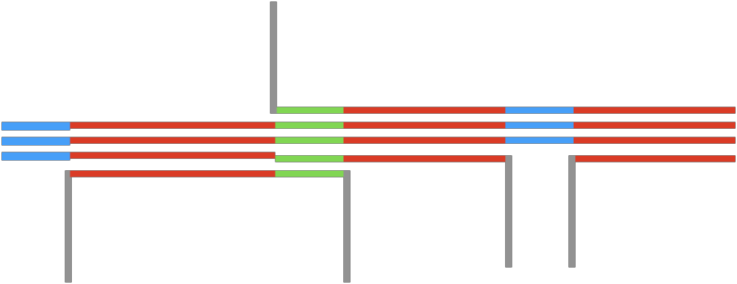
Let us see the time-evolution of the string segments of various kinds. From the left panel of Fig. 9, we compute the lengths of strings with $n_{1}=1$ as $L_{\rm ng}$, which measures the total length of the non-global strings. We also compute $L_{n_{2}}$, the length of the $\phi_{1}$-string segment which is accompanied by the $\phi_{2}$-strings with $n_{2}$. In Fig. 11, we show the time-evolution of the fractions,

The results are averaged over ten realizations and the error bars indicate the standard deviation. In this plot, the red curve shows the time-evolution of $R_{4}$. As it corresponds to the length of the compensated strings, we call it $R_{c}$ in the following. At late times, we find that about $60\%$ of the total non-global strings settle into the compensated strings. This result is rather surprising in viewing the complicated reconnection processes in the 3+1 D spacetime discussed in the previous section. In the 2+1 D simulation Hiramatsu et al. 2020, the fraction $R_{c}$ settles to $R_{c}\sim 0.8$ at the end of the simulation. The reduction of $R_{c}$ from $R_{c}\sim 0.8$ (in 2+1 D) to $R_{c}\sim 0.6$ (in 3+1 D) shows the effects of the complicated reconnection processes which make the combination process less efficient.

In addition to the compensated/uncompensated strings, there are many $\phi_{2}$-strings which are not accompanied by the $\phi_{1}$-strings. Those are the global strings, i.e., $n_{1}=0$. In the simulations, we find no global strings with $n_{2}>1$. To see the fraction of the global strings, we compute the length of the global string, $L_{\rm g}$, and define the fractions,

Here, the total string length is defined by

In Fig. 12, we show the time-evolution of the fractions. The figure shows that the string-network is dominated by the global strings although the fraction decreases at late times. The latter fact indicates that some of the global strings are absorbed by the uncompensated strings to form the compensated strings, and some of them are reconnected with each other to form loops.¹³¹³ 13 The reconnection and the loop formation of the global strings with $n_{2}=1$ take place in the usual way, regardless of the existence of $\phi_{1}$-strings. Hence, the global strings can disappear faster than the non-global strings.

Let us discuss the time-evolution of the winding numbers of the gauge-invariant NG mode, $N_{\mathrm{dw}}$, defined in Eq. (24). As we will discuss in the next section, the strings with $|N_{\mathrm{dw}}|>1$ potentially cause the axion domain-wall problem if they remain abundantly at late times. In the 2+1 D simulation in Hiramatsu et al. 2020, we found that the number of the strings with $|N_{\mathrm{dw}}|>1$ vanishes at late times. If this is the case, the axion model based on the present set up can be free from the axion domain-wall problem (see discussion in Sec. V). In the 3+1 D, however, the string combination processes are less efficient, and hence, it is imperative to estimate how large fractions of the strings have $|N_{\mathrm{dw}}|>1$ at late times in the 3+1 D simulation.

To compare with the results of the 2+1 D simulation, we compute the ratio,

in 3+1 D, where $L_{\rm others}$ is the total length of the strings with $|N_{\mathrm{dw}}|>1$.¹⁴¹⁴ 14 As mentioned earlier, no global strings with $n_{2}>1$ are formed, and hence, the global strings do not contribute to $L_{\mathrm{others}}$. This quantity is analogous to $R_{\mathrm{dw}}$ in Hiramatsu et al. 2020. In Fig. 13, we show the time-evolution of $R_{\mathrm{dw}}$ and $R_{c}$. The figure shows that the $R_{\mathrm{dw}}$ is suppressed over the simulation time, but it does not vanish at late times. The non-vanishing $R_{\mathrm{dw}}$ is due to the complexity of the string network evolution in the 3+1 D space-time.

In the figure, we also show the evolution of the rescaled fraction,

just for convenience. As $L_{\mathrm{tot}}$ is dominated by the contribution of the global strings, $R_{\mathrm{others}}$ is more suitable to see the fraction of the strings which have non-trivial NG winding around the non-global strings.

A caveat here is that $R_{\mathrm{dw}}$ and $R_{\mathrm{others}}$ do not count the uncompensated strings with $|N_{\mathrm{dw}}|>1$ precisely. In the 2+1 D simulation, the strings are point-like objects in the 2 D space. In this case, $R_{\mathrm{dw}}$ can be defined as the number fraction of the separate strings with $|N_{\mathrm{dw}}|>1$. In the 3+1 D simulation, on the other hand, the strings are connected as a network, and hence, the number of the $\phi_{2}$-strings, or the winding number $n_{2}$, changes along a $\phi_{1}$-string. This is the reason why we define the various fractions based on the length of the segments in Eqs. (33), (34), (36), and (37). Besides, the winding numbers of the segments are determined by counting the number of $\phi_{2}$-strings with $n_{2}=1$ along a $\phi_{1}$-string within $4\eta_{1}^{-1}$. Thus, for example, $R_{n_{2}}$ is contaminated by the segments with $n_{2}^{\prime}\neq n_{2}$, when the $\phi_{2}$-string around the $\phi_{1}$-string is loosely bounded or when there are some $\phi_{2}$-strings in the vicinity accidentally. Therefore, $R_{\mathrm{dw}}$ should be taken as an upper limit of the fraction of the segment with $N_{\mathrm{dw}}>1$, since some portion of $R_{3,4,5}$ which contribute to $|N_{\mathrm{dw}}|\leq 1$ are counted as $R_{\mathrm{dw}}$.¹⁵¹⁵ 15 As $R_{3}+R_{4}+R_{5}\gg R_{\mathrm{dw}}$, the relative uncertainty of $R_{\mathrm{dw}}$ caused by the contamination is larger than that of $R_{3}+R_{4}+R_{5}$ (see also the Appendix A).

Finally, let us show the parameter dependence. In Fig. 14, we show the time-evolution of $R_{c},~R_{\rm dw}$ and $R_{\rm others}$ for $\eta_{2}/\eta_{1}=0.75,~0.50,~0.25$ (from left to right). We observe the increase of $R_{c}$ for a smaller $\eta_{2}/\eta_{1}$. This shows that more uncompensated strings are bounded into the compensated strings with $N_{\mathrm{dw}}=0$ thanks to more abundant global strings at the phase transition of $\phi_{2}$ for $\eta_{2}\ll\eta_{1}$. On the other hand, we do not observe significant tendencies on $\eta_{2}/\eta_{1}$ for $R_{\rm dw}$ and $R_{\rm others}$ compared with the increase of $R_{c}$. These results indicate that $R_{\mathrm{dw}}$ and $R_{\rm others}$ could have sizable contributions from the contamination discussed above.

We also show dependence on the charge ratio. Fig. 15 shows the time-evolution of $R_{c},~R_{\rm dw}$ and $R_{\rm others}$ for $q_{2}=2,~3,~4$ (from left to right). We observe that $R_{c}$ decreases for a larger $q_{2}/q_{1}$. This is expected because the uncompensated strings require more $\phi_{2}$-strings to evolve into the compensated strings for a larger $q_{2}/q_{1}$.

Finally, let us comment that the case with the opposite charge ratio, $q_{2}/q_{1}=1/4$, while keeping the ratio of the VEVs, $\eta_{2}/\eta_{1}=0.25$. In this case, we find that the strings with $(n_{1},n_{2})=(1,0)$ and $(0,1)$ remain at the end of the simulations, although we do not show the results. Similar results are also obtained in the 2+1 D simulation. This behavior can be understood that we need four $\phi_{1}$-strings and one $\phi_{2}$-string to form the compensated string. This is difficult as $\phi_{1}$-strings are formed at $T\sim\eta_{1}$, while the $\phi_{2}$-strings are formed at much lower temperature, $T\sim\eta_{2}$. As the global strings, formed at $T\sim\eta_{2}$, have $N_{\mathrm{dw}}=4$, we expect $R_{\mathrm{dw}}$ is close to 1, for a model with $\eta_{1}>\eta_{2}$ and $q_{1}>q_{2}$.

References

- Hiramatsu et al. (2020) T. Hiramatsu, M. Ibe, and M. Suzuki, JHEP 02, 058 (2020), arXiv:1910.14321 [hep-ph] .
- Peccei and Quinn (1977a) R. D. Peccei and H. R. Quinn, Phys. Rev. Lett. 38, 1440 (1977a).
- Peccei and Quinn (1977b) R. D. Peccei and H. R. Quinn, Phys. Rev. D16, 1791 (1977b).
- Weinberg (1978) S. Weinberg, Phys. Rev. Lett. 40, 223 (1978).
- Wilczek (1978) F. Wilczek, Phys. Rev. Lett. 40, 279 (1978).
- Barr et al. (1982) S. M. Barr, X. C. Gao, and D. Reiss, Phys. Rev. D26, 2176 (1982).
- Choi and Kim (1985) K. Choi and J. E. Kim, Phys. Rev. Lett. 55, 2637 (1985).
- Fukuda et al. (2017) H. Fukuda, M. Ibe, M. Suzuki, and T. T. Yanagida, Phys. Lett. B771, 327 (2017), arXiv:1703.01112 [hep-ph] .
- Fukuda et al. (2018) H. Fukuda, M. Ibe, M. Suzuki, and T. T. Yanagida, JHEP 07, 128 (2018), arXiv:1803.00759 [hep-ph] .
- Ibe et al. (2018) M. Ibe, M. Suzuki, and T. T. Yanagida, JHEP 08, 049 (2018), arXiv:1805.10029 [hep-ph] .
- Hawking (1987) S. W. Hawking, Moscow Quantum Grav.1987:0125, Phys. Lett. B195, 337 (1987).
- Lavrelashvili et al. (1987) G. V. Lavrelashvili, V. A. Rubakov, and P. G. Tinyakov, JETP Lett. 46, 167 (1987), [Pisma Zh. Eksp. Teor. Fiz.46,134(1987)].
- Giddings and Strominger (1988) S. B. Giddings and A. Strominger, Nucl. Phys. B307, 854 (1988).
- Coleman (1988) S. R. Coleman, Nucl. Phys. B310, 643 (1988).
- Gilbert (1989) G. Gilbert, Nucl. Phys. B328, 159 (1989).
- Banks and Seiberg (2011) T. Banks and N. Seiberg, Phys. Rev. D83, 084019 (2011), arXiv:1011.5120 [hep-th] .
- Nielsen and Olesen (1973) H. B. Nielsen and P. Olesen, Nucl. Phys. B61, 45 (1973), [,302(1973)].
- Bezerra de Mello et al. (2003) E. R. Bezerra de Mello, Y. Brihaye, and B. Hartmann, Phys. Rev. D 67, 124008 (2003), arXiv:hep-th/0302212 .
- Hill et al. (1988) C. T. Hill, A. L. Kagan, and L. M. Widrow, Phys. Rev. D 38, 1100 (1988).
- Garaud and Babaev (2014) J. Garaud and E. Babaev, Phys. Rev. B 89, 214507 (2014), arXiv:1403.3373 [cond-mat.supr-con] .
- Vincent et al. (1998) G. Vincent, N. D. Antunes, and M. Hindmarsh, Phys. Rev. Lett. 80, 2277 (1998), arXiv:hep-ph/9708427 [hep-ph] .
- Moore et al. (2002) J. N. Moore, E. P. S. Shellard, and C. J. A. P. Martins, Phys. Rev. D65, 023503 (2002), arXiv:hep-ph/0107171 [hep-ph] .
- Salmi et al. (2008) P. Salmi, A. Achucarro, E. J. Copeland, T. W. B. Kibble, R. de Putter, and D. A. Steer, Phys. Rev. D77, 041701 (2008), arXiv:0712.1204 [hep-th] .
- Achucarro and de Putter (2006) A. Achucarro and R. de Putter, Phys. Rev. D74, 121701 (2006), arXiv:hep-th/0605084 [hep-th] .
- Yamaguchi et al. (1999) M. Yamaguchi, M. Kawasaki, and J. Yokoyama, Phys. Rev. Lett. 82, 4578 (1999), arXiv:hep-ph/9811311 [hep-ph] .
- Yamaguchi et al. (2000) M. Yamaguchi, J. Yokoyama, and M. Kawasaki, Phys. Rev. D61, 061301 (2000), arXiv:hep-ph/9910352 [hep-ph] .
- Yamaguchi (1999) M. Yamaguchi, Phys. Rev. D60, 103511 (1999), arXiv:hep-ph/9907506 [hep-ph] .
- Yamaguchi and Yokoyama (2002) M. Yamaguchi and J. Yokoyama, Phys. Rev. D66, 121303 (2002), arXiv:hep-ph/0205308 [hep-ph] .
- Yamaguchi and Yokoyama (2003) M. Yamaguchi and J. Yokoyama, Phys. Rev. D67, 103514 (2003), arXiv:hep-ph/0210343 [hep-ph] .
- Hiramatsu et al. (2013) T. Hiramatsu, Y. Sendouda, K. Takahashi, D. Yamauchi, and C.-M. Yoo, Phys. Rev. D88, 085021 (2013), arXiv:1307.0308 [astro-ph.CO] .
- Higaki et al. (2016) T. Higaki, K. S. Jeong, N. Kitajima, T. Sekiguchi, and F. Takahashi, JHEP 08, 044 (2016), arXiv:1606.05552 [hep-ph] .
- Hindmarsh et al. (2019) M. Hindmarsh, J. Lizarraga, J. Urrestilla, D. Daverio, and M. Kunz, Phys. Rev. D99, 083522 (2019), arXiv:1812.08649 [astro-ph.CO] .
- Chatterjee et al. (2020) C. Chatterjee, T. Higaki, and M. Nitta, Phys. Rev. D 101, 075026 (2020), arXiv:1903.11753 [hep-ph] .
- Lazarides and Shafi (1982) G. Lazarides and Q. Shafi, Phys. Lett. B115, 21 (1982).
- Kawasaki and Nakayama (2013) M. Kawasaki and K. Nakayama, Ann. Rev. Nucl. Part. Sci. 63, 69 (2013), arXiv:1301.1123 [hep-ph] .
- Kim (1979) J. E. Kim, Phys. Rev. Lett. 43, 103 (1979).
- Shifman et al. (1980) M. A. Shifman, A. I. Vainshtein, and V. I. Zakharov, Nucl. Phys. B166, 493 (1980).
- Vilenkin and Everett (1982) A. Vilenkin and A. E. Everett, Phys. Rev. Lett. 48, 1867 (1982).
- Hiramatsu et al. (2012) T. Hiramatsu, M. Kawasaki, K. Saikawa, and T. Sekiguchi, Phys. Rev. D85, 105020 (2012), [Erratum: Phys. Rev.D86,089902(2012)], arXiv:1202.5851 [hep-ph] .