Predictions of Quantum Gravity
in Inflationary Cosmology:
Effects of the Weyl-squared Term
Damiano Anselmi1,2,a, Eugenio Bianchi3,4,b and Marco Piva5,c
1Dipartimento di Fisica “Enrico Fermi”, Università di Pisa, Largo B. Pontecorvo 3, 56127 Pisa, Italy
2INFN, Sezione di Pisa, Largo B. Pontecorvo 3, 56127 Pisa, Italy
3Institute for Gravitation and the Cosmos, The Pennsylvania State University, University Park, Pennsylvania 16802, USA
4Department of Physics, The Pennsylvania State University, University Park, Pennsylvania 16802, USA
5National Institute of Chemical Physics and Biophysics, Rävala 10, Tallinn 10143, Estonia
adamiano.anselmi@unipi.it, bebianchi@gravity.psu.edu, cmarco.piva@kbfi.ee
Abstract
We derive the predictions of quantum gravity with fakeons on the amplitudes and spectral indices of the scalar and tensor fluctuations in inflationary cosmology. The action is plus the Weyl-squared term. The ghost is eliminated by turning it into a fakeon, that is to say a purely virtual particle. We work to the next-to-leading order of the expansion around the de Sitter background. The consistency of the approach puts a lower bound () on the mass of the fakeon with respect to the mass of the inflaton. The tensor-to-scalar ratio is predicted within less than an order of magnitude ( to the leading order in the number of -foldings ). Moreover, the relation is not affected by the Weyl-squared term. No vector and no other scalar/tensor degree of freedom is present.
1 Introduction
Inflation is a theory of accelerated expansion of the early universe [1, 2, 3, 4, 5, 6, 7, 8], which accounts for the origin of the present large-scale structure. It explains the approximate isotropy of the cosmic microwave background radiation and allows us to study the quantum fluctuations as sources of the cosmological perturbations that seed the formation of the structures of the cosmos [9, 10, 11, 12, 13, 14, 15]. It also provides a rich environment where we can develop knowledge that might allow us to establish a nontrivial connection between high-energy physics and the physics of large scales.
Inflationary cosmology is often studied with the help of a matter field that drives the expansion by rolling down a potential (for reviews, see [16, 17]). Alternatively, gravity itself can drive the expansion, as in the Starobinsky model [2] and the theories [18, 19]. The predictions end up depending strongly on the model, specifically the choices of and . In single-field slow-roll inflation, potentials with a plateau lead to a scalar power spectrum that is compatible with current observations [20, 21].
In particular, the Starobinsky model works well at the phenomenological level. However, once is introduced, it is hard to justify why the square of the Weyl tensor is not included as well, since it has the same dimension in units of mass. We can spare the other quadratic combinations, such as and , since they are related to and by algebraic identities and the Gauss-Bonnet theorem. Thus, we are lead to consider the action
| (1.1) |
which we briefly refer to as “ theory”. The trouble with (1.1) is that the term is normally responsible for the presence of ghosts. Immediate ways out are to expand the physical quantities in powers of [22], which is equivalent to assume that the ghosts are very heavy, and/or restrict to situations where the ghosts are short-lived. This approach amounts to “living with ghosts” [23], but does not eliminate the problem.
If we want to work with the theory, we must explain how to treat in order to remove the ghosts, at least perturbatively and at the level of the cosmological perturbations. Here we use the procedure of eliminating them in favor of purely virtual particles [24, 25]. This procedure originates in high-energy physics, where the requirements of locality, renormalizability and unitarity result in consistency contraints on perturbative quantum field theory.
The simplest way to think of the idea is as follows. A normal particle can be real or virtual, depending on whether it is observed or not. As far as we know, a particle that is always real does not exist. What about a particle that is always virtual and can never become real? We can think of it as a purely virtual quantum [26] or a fake particle, i.e., a particle that mediates interactions among other particles, but is invisible to our detectors. And by that we mean invisible in principle, not just in practice.
Perturbative quantum gravity can be formulated as a unitary theory of scattering if the action (1.1) is quantized in a new way [24], by eliminating the would-be ghost in favor of a purely virtual particle, called fakeon [25]. In the expansion around flat space, the fakeon is introduced by replacing the Feynman prescription (for a pole of the free propagator) with an alternative prescription that allows us to project the corresponding degree of freedom away consistently with the optical theorem. This means that the loop corrections are unable to resuscitate the degree of freedom back. Moreover, the prescription is compatible with renormalizability [24, 25]. A fakeon mediates interactions, but does not belong to the spectrum of asymptotic states. In this sense it is a “fake degree of freedom.” Note that it removes a ghost at the fundamental level, without advocating its irrelevance for practical purposes. Incidentally, the calculations of Feynman diagrams with the fakeon prescription in quantum gravity [27, 28] are not harder than analogous calculations for the standard model.
Nevertheless, quantum field theory is formulated perturbatively, commonly around flat space. To study inflation and cosmology it is necessary to work on nontrivial backgrounds. This raises the issue of understanding purely virtual quanta in curved space. A simplification comes from the fact that in cosmology we do not need to go as far as computing loop corrections, as argued in ref. [29], although we have to study the quantum fluctuations. In this paper, we show that we can work with the classical limit of the fakeon prescription/projection, which amounts to taking the average of the retarded and advanced potentials as Green function for the fake particles [30],
| (1.2) |
combined with a certain wealth of knowledge on how to use this formula and interpret its consequences. Note that the quantum fakeon prescription cannot be inferred from (1.2), because (1.2) is not a good propagator in Feynman diagrams [26].
As said, the predictions of the popular models of inflation are model dependent. On the other hand, in high-energy physics the constraints of locality, unitarity and renormalizability leave room for a limited class of interactions, scalar potentials, and so on, to the extent that the theory of quantum gravity emerging from the idea of fake particle is essentially unique (when matter is switched off) and contains just two independent parameters more than Einstein gravity. They can be identified as the masses and of a scalar field (the inflaton) and a spin-2 fakeon . The triplet graviton-scalar-fakeon exhausts the set of degrees of freedom of the theory. From the cosmological point of view the physical modes are the usual curvature perturbation and the tensor fluctuations. The extra degrees of freedom are turned into fake ones and projected away. In particular, no vector fluctuations, or additional scalar and tensor fluctuations survive.
We show that the consistency of the picture in curved space leads to a lower bound on the mass of the fakeon with respect to the mass of the inflaton. To the next-to-leading order, the amplitude and the spectral index of the scalar fluctuations depend only on (and the number of -foldings). Instead, the amplitude and the spectral index of the tensor fluctuations do depend on . The bound narrows the window of allowed values of and the tensor-to-scalar ratio to less than one order of magnitude and makes the predictions quite precise, even before knowing the actual values of and .
Inflationary cosmology in higher-derivative gravity with ghosts have been studied in refs. [31, 32]. Typically, the ghost sector is quantized by means of negative norms. Extra spectra are predicted, which may or may not be suppressed on superhorizon scales. Inflation has been considered in nonlocal theories of gravity as well [33], where the classical action contains infinitely many free parameters. The cosmological perturbations in those scenarios have been studied in [34].
The gain achieved by means of fakeons is that no ghosts are present and the number of independent parameters is kept to a minimum. Whenever there is an overlap, we find agreement with the results derived in the other approaches. This occurs, for example, when or are sufficiently small to suppress the effects of the fakeons in our theory and the effects of the ghosts in the theories of refs. [32], where is the value of the Hubble parameter during inflation. Even when or are not large, we can still relate some results, due to the universality of the low-energy expansion. For example, we can do so for any quantity that has a convergent, resummable expansion for small or . In the limit , the results we find agree with those of the theory [18, 35].
We make the calculations in two frameworks and show that the final results match. In the first approach, which we call inflaton framework, the scalar field is introduced explicitly to eliminate the term, while the term is unmodified. The scalar potential coincides with the Starobinsky one. In the second approach, which we call geometric framework, both and are present. The term does not affect the FLRW metric, so in both approaches the background metric coincides with the one of the Starobinsky theory. The differences arise in the action of the fluctuations over the background. The map relating the two frameworks is a field-dependent conformal transformation, combined with a time reparametrization. A third formulation, where the scalar and a spin-2 fakeon are introduced explicitly in order to eliminate both higher-derivative terms and is also available [28], but will not be studied here.
The paper is organized as follows. In section 2, we briefly review the formulation of quantum gravity with fakeons and present the two frameworks just mentioned. In section 3, we study the tensor and scalar fluctuations in the inflaton framework. The fakeon projection, which allows us to make sense of the term , is briefly introduced in section 2 and discussed in detail in section 4. In section 5, we make the calculations in the geometric framework. In section 6, we study the vector fluctuations and show that they are projected away altogether at the quadratic level. Section 7 contains the summary of our predictions and section 8 contains the conclusions. In appendix A, we derive the map relating the inflaton framework to the geometric framework and show that the results agree. In appendix B we show that the curvature perturbation can be considered constant on superhorizon scales for adiabatic fluctuations of the energy-momentum tensor.
2 Quantum gravity with fakeons
In this section we introduce the theory and the two frameworks we are going to work with. We begin by recalling a few basic features of the fakeons. Being purely virtual quanta, they are particles that mediate interactions, but do not belong to the physical spectrum of asymptotic states. Expanding around flat space, they are introduced by means of a new quantization prescription for the poles of the free propagators [24], alternative to the Feynman prescription. The physical subspace is obtained by projecting the fake degrees of freedom away. The theory is unitary in , where the optical theorem holds. What makes the projection consistent to all orders [25] is that the fakeon prescription does not allow the loop corrections to resuscitate back the states that have been projected away.
The prescription makes sense irrespective of the sign of the residue at the pole of the propagator. Yet, it requires that the real part of the squared mass be positive. Indeed, fakeons cannot cure tachyons, but only ghosts. The no-tachyon condition is the main requirement we have to fulfill and its analogue on nontrivial backgrounds is going to play an important role.
The projection must also be performed at the classical level. An action like (1.1) is physically unacceptable as the classical limit of quantum gravity, because it has undesirable solutions. Yet, (1.1) is the starting point to formulate quantum gravity as a quantum field theory. It is local and provides the Feynman rules that allow us (together with the Feynman prescription for physical particles and the fakeon prescription for fake particles), to calculate the loop diagrams and the matrix. An action of this type is called “interim” classical action [30].
The true classical action is obtained from the interim classical action by projecting the fake degrees of freedom away. At the classical level, the projection is achieved by means of the classical limit of the fakeon prescription. Precisely, is obtained by: () solving the field equations of the fakeons (derived from ) by means of the fakeon Green function; and () inserting the solutions back into . In the perturbative expansion around flat space, the fakeon Green function is the arithmetic average of the retarded and advanced potentials [30]. We will see that this piece of information is enough to derive the fakeon Green function on nontrivial backgrounds.
The plan of the paper is to calculate the effects of inflationary cosmology on the fluctuations of the cosmic microwave background radiation at the quadratic level. Since we do not need to work out loop corrections, we can quantize the projected action , rather than projecting the quantum version of . This simplification saves us a lot of effort.
The good feature of is that it no longer contains the fake degrees of freedom, by construction, so in principle it can be quantized with the usual methods. The nontrivial counterpart is that is not fully local, due to the nonlocal remnants left by the fakeon projection. Because of this, the quantization of is not as simple as usual, also taking into account that we must perform it on a nontrivial background. However, in a variety of lucky cases, which include those studied in this paper, it is possible to treat the nonlocal sector of in a relatively simple way and extract physical predictions with the procedure described above, either because the nonlocal sector of does not affect the quantities we are interested in, or because it affects them only at higher orders.
Summarizing, the simplest way to proceed, which we adopt in the paper, is as follows. First, we work out the classical action of quantum gravity, by projecting the interim action . Second, we quantize with the usual methods, paying special attention to the nonlocal sector, anticipating that in the end it does not create too serious difficulties.
Now we give the interim classical actions of quantum gravity in the two approaches we study in the paper. The projection and the quantization of will be performed in the next sections, after expanding around the de Sitter background.
The higher-derivative form of the interim classical action is
| (2.1) |
where denotes the Weyl tensor, is the Planck mass, are the matter fields and is the action of the matter sector. The no-tachyon condition (i.e., the requirement that the free propagator around flat space does not have tachyonic poles) determines the signs in front of and .
The degrees of freedom of the gravitational sector are the graviton, a scalar field of mass and a spin-2 fakeon of mass . The reason why must be quantized as a fakeon is that the residue of the free propagator has the wrong sign at the pole, so the Feynman prescription would turn it into a ghost, causing the violation of unitarity. On the other hand, can be quantized either as a fakeon or a physical particle, because the residue at the pole has the correct sign. In this paper, we assume that is a physical particle (the inflaton).
For simplicity, we have omitted the cosmological term in (2.1). We will do the same throughout the paper. Once it is included, the theory is manifestly renormalizable, like Stelle’s theory [36], because the fakeon prescription does not modify the ultraviolet divergences [24, 25].
With the help of an auxiliary field , we can write in the equivalent form
| (2.2) | |||||
Making the Weyl transformation
| (2.3) |
where , we can diagonalize the quadratic part and obtain the new action
| (2.4) |
where
| (2.5) |
and
| (2.6) |
is the Starobinsky potential. The action (2.4) is not manifestly renormalizable. In fact, it is as renormalizable as (2.1) – once the cosmological term is reinstated –, because it is related to (2.1) by a (perturbative and nonderivative) field redefinition.
The geometric framework is defined by the interim actions (2.1) or (2.2), while the inflaton framework is defined by (2.4). In the rest of the paper, we switch the matter sector off. If needed, its effects can be studied along the guidelines outlined in the next sections. We do not review the details on the parametrizations of the fluctuations and their transformations under diffeomorphisms, which are easy to find in the literature (see for example [17, 18]).
3 Inflaton framework (scalar)
In this section, we study the tensor and scalar fluctuations in the inflaton framework. The action is (2.4), with the potential (2.6). The Friedmann equations are
| (3.1) |
where . We define the usual quantities
| (3.2) |
where is the Hubble parameter.
The de Sitter limit is the one where is approximately constant. It is easy to show that the constant value it tends to is . Indeed, in the first equation (3.1) gives . On the other hand, if we insert (and so ) in the third equation (3.1) we obtain , which has two solutions: and . The first possibility gives the trivial case, since , in the second equation (3.1) give . The second possibility is the right one, since , in the second equation (3.1) give .
The expansion around the de Sitter background is an expansion in powers of . This can be proved by studying the solution of the equations (3.1) around the de Sitter metric. Leaving the details to appendix A, here we just mention the properties that we need to proceed. It is possible to show that and
| (3.3) |
In other words, each time derivative raises the order by , so the expansion in powers of is also an expansion of slow time dependence. Moreover, we have
| (3.4) | |||||
(see formulas (A.7), suppressing bars). The last line is the expansion of , where is the conformal time, defined by
| (3.5) |
with the initial condition chosen to have in the de Sitter limit .
3.1 Tensor fluctuations
To study the tensor fluctuations, it is convenient to parametrize the metric as
| (3.6) |
where and are the graviton modes.
Let denote the Fourier transform of with respect to the coordinate , where is the space momentum. The quadratic Lagrangian obtained from (2.4) is
| (3.7) |
plus an identical contribution for , where . To simplify the notation, we understand that stands for , for , etc. We extend this convention to mixed products such as , which can be interpreted either as or .
It is possible to eliminate the higher derivatives by considering the extended Lagrangian
| (3.8) |
where
| (3.9) |
Here , are functions to be determined, and , which may stand for or , denotes an auxiliary field. The equivalence of and is due to the fact that when is replaced by the solution of its own field equation. The higher derivatives disappear in the sum , because the term proportional to cancels out.
Next, we perform the field redefinitions
| (3.10) |
where and are other functions to be determined. We use the freedom to choose , , and to write in a convenient form, such that it contains a unique, nonderivative term mixing and . Specifically, we reduce the Lagrangian to the form
| (3.11) |
where
| (3.12) |
and , , and are other functions of time, while is constant and has the dimension of a mass. Since is going to be positive, is the fakeon and is the physical excitation, up to the mixing due to .
The fakeon projection amounts to solving the field equations by means of the fakeon prescription and inserting the solution back into . In all the cases considered here, this is achieved by determining the solution of as the arithmetic average of the retarded and advanced potentials, where is an operator of the form
| (3.13) |
being functions of time. A certain detour allows us to get to the results we need here without even knowing the explicit expression of , which is derived in section 4, where the projection is discussed in detail.
The constant is in principle arbitrary, but a remarkable choice, , makes vanish in the de Sitter limit. There, and decouple and
| (3.16) |
It is relatively straightforward to derive the power spectrum of the fluctuations in this limit. The equation of motion is
| (3.17) |
As said, we need to solve it by means of the fakeon prescription and insert the solution back into the action. Since (3.17) is homogeneous and -independent, the solution is just .
Using , formula (3.10) gives , so we obtain a Mukhanov action
that coincides with the one of Einstein gravity with a scalar field, apart from the overall factor. The two-point function in the de Sitter limit is
| (3.18) |
where
Details on the derivation of (3.18) are given below. Formula (3.18) makes us already appreciate that the result depends on the mass of the fakeon in a nontrivial way.
Quasi de Sitter expansion
Formulas (3.14) and (3.15) are exact, i.e., they do not assume small. From now on, we work to the first order in , where we can use approximate formulas. Observe that (3.14) and (3.15) depend on , , and (through ). However, the last three quantities are related by (3.4), so we can eliminate one of them. The price of this is that we introduce terms proportional to , which are unnecessary at this level. It is possible to avoid it by switching to a slightly different parametrization. Specifically, if we choose
| (3.19) |
and
| (3.20) |
we find the Lagrangian
| (3.21) |
The equation of motion is now
| (3.22) |
where
| (3.23) |
Anticipating that the solution for is of order , we have dropped higher-order terms proportional to , from (3.22). Let denote the fakeon Green function , i.e., the solution of defined by the fakeon prescription (see section 4). Then the solution of (3.22) can be written as
| (3.24) |
Inserting this expression into the Lagrangian (3.21), we can see that the nonlocal contribution due to is of order , so we can drop it. The projected Lagrangian is
| (3.25) |
Power spectrum and spectral index
Formula (3.27) tells us that the conjugate momentum of is , so after turning , into operators , , we impose the equal time quantization condition
| (3.28) |
where we have reinstated the subscripts . As usual, we write the Fourier decomposition
| (3.29) |
where and are creation and annihilation operators.
The limit of (3.27) allows us to define the Bunch-Davies vacuum state . From formula (3.27), we see that the only difference with respect to the result obtained in the de Sitter limit is a rescaling of . Thus, we require
| (3.30) |
Using the condition (3.30), we can work out the modes and obtain
| (3.31) |
having used the third formula of (3.4), where are the Hankel functions. For the purpose of computing the power spectrum, we need to work out the leading behavior in the superhorizon limit . There we have
| (3.32) |
The redefinitions (3.10) tell us that to compute the two-point function we also need the fakeon , which is given by formula (3.24). While the general discussion of the fakeon Green function is left to section 4, here we can quickly get to the result we need as follows. In the superhorizon limit we can ignore the term proportional to in the expression (3.20) of . Once we do this, we can commute and in (3.24), because the commutator gives corrections of higher orders in . Moreover, recalling that , because solves the Mukhanov equation of the projected Lagrangian of formula (3.25), just multiplies by . Collecting these facts, we have, in the superhorizon limit and discarding higher orders,
that is to say,
| (3.33) |
The power spectrum of each graviton polarization is defined by
| (3.34) |
The two-point function can be evaluated in the superhorizon limit from (3.10), (3.31) and (3.33). We find
where is the digamma function.
The power spectrum of the tensor fluctuations, matched with the usual conventions, is . Replacing by , where is a reference scale, it is common to write
| (3.35) |
where and are called amplitude and spectral index (or tilt), respectively. We find
| (3.36) |
where is the Euler-Mascheroni constant and we have used the first formula of (3.4) to eliminate .
3.2 Scalar fluctuations
Now we study the scalar fluctuations in the inflaton framework. We work in the comoving gauge, where the fluctuation is set to zero and the metric reads
| (3.37) |
After Fourier transforming the space coordinates, (2.4) gives the quadratic Lagrangian
| (3.38) | |||||
As before, stands for , for , and so on.
Since appears algebraically, we eliminate it by means of its own field equation. We remain with a Lagrangian that depends only on and . The field redefinitions
| (3.39) |
allow us to decompose as
| (3.40) |
where is the sum of a term proportional to plus one proportional to . In addition, vanishes in the de Sitter limit.
We do not give the full expression of here, but stress that after the redefinition (3.39) it admits a series expansion in powers of and . In particular,
where is defined in (3.19). As before, is the fakeon and is the physical excitation.
Quasi de Sitter expansion
In the de Sitter limit , we find
| (3.41) |
where
Note that and the coefficient of in (3.41) are positive definite.
Again, we see that the fakeon decouples. Its own equation of motion sets it to zero, so the Lagrangian of coincides with the usual Mukhanov expression, normalization included. This means that the power spectrum of the scalar fluctuations coincides with the one of Einstein gravity in this limit.
To order , we find
| (3.42) |
Since the equation of motion implies , remains the one of formula (3.41) to the order we are considering. Moreover, after integrating out, the projected Lagrangian is just , since the -dependent corrections are .
From , we can derive the Mukhanov action by following the steps from (3.26) to (3.32), with the replacements , and , where
| (3.43) |
Recalling that in the comoving gauge the curvature perturbation coincides with , we can derive the power spectrum , defined by
| (3.44) |
Inserting the solution for into the left formula of (3.39), we find
| (3.45) |
where the amplitude and the spectral index are
| (3.46) | |||||
| (3.47) |
respectively. We see that the mass of the fakeon does not affect the result to the order we are considering.
Finally, from (3.36) we derive the tensor-to-scalar ratio
| (3.48) |
4 The fakeon projection
In this section we discuss the fakeon projection, starting from the tensor fluctuations. The Lagrangian of formula (3.21) leads to the equation of motion (3.22). The fakeon Green function is the solution of , defined by the fakeon prescription, where is given in formula (3.23). For the purposes of this paper, it is sufficient to invert in the de Sitter limit , where is treated as a constant. We keep generic to make the discussion easily adaptable to the geometric framework. We will use the information that is in the de Sitter limit (in the inflaton framework) only later.
It is convenient to switch to a symmetric operator by noting that
| (4.1) |
We want to prove that the fakeon solution of
| (4.2) |
is
| (4.3) |
where is the sign function, denotes the Bessel function of the first kind and
| (4.4) |
In principle, we could add solutions of the homogeneous equation, which are the functions , multiplied by constants. The job of the projection is to determine those constants uniquely. Because it comes from quantum field theory, the fakeon projection is known perturbatively around flat space, in four-momentum space. However, a notion of four-momentum is not immediately available in curved space.
Fortunately, there are three limits where is known, which are , and constant. The limit gives the flat-space case once we switch to conformal time. The limit gives the flat-space case if we keep the cosmological time. The case constant is precisely flat space, but is not relevant here, since we are interested in the de Sitter background. Hence, necessary conditions are that the solution (4.3) reduces to the known expressions [30, 37] in both cases and . Any of these two conditions is also sufficient. The other condition can be seen as a consistency check.
Switching to conformal time , equation (4.2) can be written as
For large we obtain
| (4.5) |
Solving it by means of the arithmetic average of the retarded and advanced potentials, we find [30, 37]
| (4.6) |
As said, the most general solution of (4.2) is equal to (4.3) plus solutions of the homogeneous equation, multiplied by constant coefficients and . Now we know that those coefficients must vanish, to match (4.6) for large. This proves that (4.3) is the correct fakeon Green function.
A consistency check is given by the limit . There, (4.2) turns into an equation similar to (4.5), provided we keep the cosmological time instead of switching to . Consequently, the solution (4.3) must tend to [30, 37]
| (4.7) |
It is easy to check that this is indeed the limit of (4.3).
From (4.1) we derive the fakeon Green function
| (4.8) |
4.1 Consistency condition
We have determined the fakeon Green function in curved space by referring to two situations where the problem becomes a flat-space one, which are and . As mentioned in the introduction, purely virtual particles are subject to a consistency (no-tachyon) condition in flat-space, i.e., their squared mass should be positive. Formula (4.6) shows that this requirement is always satisfied for , while formula (4.7) shows that it is satisfied for if is real. Recalling that is in the inflaton framework, the condition reads
| (4.9) |
which is a lower bound on the mass of the fakeon with respect to the mass of the inflaton. When (4.9) holds, the oscillating behavior of (4.7) suppresses the contributions with
One may wonder if it is meaningful to impose a condition stronger than (4.9), for example require that the time-dependent squared mass be positive for all values of . To discuss this issue, let us consider the Lagrangian that gives the fakeon Green function of formula (4.2), which is
| (4.10) |
A redefinition , , with , leaves the kinetic term invariant, but changes the squared mass. Specifically, the transformed Lagrangian reads
where
| (4.11) |
This transformation law shows that the signs of and do not have a reparametrization-independent meaning, in general, so a squared mass that becomes negative in some time interval is not necessarily a sign of a lack of consistency.
In passing, it is easy to verify that if the masses are independent of time, then the condition of positive square mass is independent of the parametrization. Indeed, if is -independent and positive, the most general reparametrization that leaves -independent has
where and are arbitrary real constants of integration. Since must be real and identically positive, must also be positive.
Summarizing, a necessary condition for the fakeon projection in the inflationary scenario is that the fakeon squared mass be positive in the superhorizon limit:
| (4.12) |
This condition also leads to (4.9) in the case of the scalar fluctuations. Indeed, consider the Lagrangian given in formula (3.41). Making the change of variables
| (4.13) |
the equation of motion takes the form
| (4.14) |
for some involved rational function of and , equal to in the superhorizon limit. Thus, (4.12) gives again the bound (4.9).
As we show in section 6, the vector fluctuations give the same bound. The same bound is also found in the geometric framework. It is conceivable that, if (4.9) were violated, the theory would predict a rather different large-scale structure of the universe, or a different scenario would have to be envisaged to produce the present situation.
The stronger requirement that be positive for every makes sense if we believe that the cosmological time plays a special role. Then we still find the bound (4.9) for the tensor fluctuations, while a stronger bound is obtained in the case of the scalar fluctuations. Studying the coefficient of in (4.14) numerically, we find that it is positive for all values of if
| (4.15) |
As soon as , there exists a finite domain where has negative values. When satisfies (4.9) but not (4.15), there is a time interval , comparable with the duration of inflation, where the fakeon Green function is “tachyonic” and its nonlocal contribution is no longer negligible.
In the rest of the paper, we take (4.9) as the consistency condition for the fakeon projection in inflationary cosmology, because it is universal and reparametrization independent. Yet, the issues just mentioned suggest that there is a chance that it might be conservative. The formulas of the power spectra do not depend on it, but (4.15) narrows the window of allowed values of the tensor-to-scalar ratio a little bit more than (4.9) (see section 7).
5 Geometric framework ()
In this section we study the geometric framework, which is sometimes known in the literature as Jordan frame. The higher-derivative equations of the background metric, derived from (2.1) with the FLRW ansatz, can be written in the simple form
| (5.1) |
where is again . It is worth to stress that , , and the cosmological time are different from those of the inflaton framework, although we denote them by means of the same symbols. The match between the two frameworks is worked out in detail in Appendix A.
The quasi de Sitter approximation of (5.1) requires , so is no longer related to in the de Sitter limit, where actually . As far as the mass is concerned, it can be either of order or of order . This means that we have two types of quasi de Sitter expansions, depending on whether or . We study the scalar and tensor fluctuations in both.
The two possibilities can also be understood as follows. The de Sitter metric is not an exact solution of the field equations of the theory . It is an exact solution in two cases: () when we ignore both and ; and () when we ignore just . In other words, the term is leading with respect to the term , while the term can either be of order or of order (as far as the fluctuations are concerned). The first case is studied by expanding in powers of with fixed. The second case is studied by expanding in powers of with fixed.
The relation between , and is
| (5.2) |
It can be found by writing down the most general expansion for in powers of , differentiating it and applying (5.1) to determine the coefficients. If needed, (5.2) can be extended to arbitrarily high orders (an asymptotic series being obtained).
5.1 : tensor fluctuations
We start from the tensor fluctuations. Parametrizing the metric as in (3.6), the quadratic Lagrangian obtained from (2.1) is
| (5.3) |
plus an identical contribution for , where
| (5.4) |
Expanding around the de Sitter background with fixed, the first nonvanishing contribution to the spectral index turns out to be . For this reason, we work out the predictions to the second order in included. Expanding the Lagrangian (5.3), we find
| (5.5) | |||||
where
The important point of (5.5) is that the unique higher-derivative term is multiplied by , so the fakeon projection can be handled iteratively. The change of variables
| (5.6) | |||||
allows us to cast the Lagrangian in the form
Since for small [as in (3.32)], the corrections of (5.6) are either or give subleading contributions in the superhorizon limit . This means that we do not need to specify them for our purposes.
At this point, it is sufficient to upgrade the steps from formula (3.26) to formula (3.32) to the appropriate order, with the substitutions , , . We find
| (5.7) |
The power spectrum of the tensor fluctuations is , with defined by (3.34). Using the definition (3.35), the amplitude and the spectral index are
| (5.8) | |||||
| (5.9) |
5.2 : scalar fluctuations
Now we discuss the scalar fluctuations in the geometric framework by expanding in powers of to the next-to-leading order with fixed. We switch directly from (2.1) to the action (2.2) (with ), to remove the higher derivatives without changing the metric that couples to matter. We isolate the background value of from its fluctuation by writing
| (5.10) |
where is defined in (5.4). The gauge invariant curvature perturbation is
| (5.11) |
We work in the spatially-flat gauge, where is an independent field and is set to zero. This means that the metric is
| (5.12) |
After Fourier transforming the space coordinates, the quadratic Lagrangian reads
| (5.13) | |||||
The field appears in (5.13) as a Lagrange multiplier, so we integrate it out by solving its own field equation and inserting the solution back into the action. So doing, we obtain a two-derivative quadratic Lagrangian for and , which we then expand around the de Sitter background by means of (5.2). Making the field redefinitions
| (5.14) |
we obtain an action that is regular for . Its limit is
We note that at this level appears algebraically and can be integrated out. This means that the fakeon projection can be handled iteratively in .
After integrating out, every dependence disappears to the first order in . In particular, if we define
| (5.15) |
the action becomes
| (5.16) |
The redefinition (3.26) with , and , where
| (5.17) |
gives the action (3.27) with . Inserting the solution for into (5.15), (5.14) and then (5.11), and using the definition (3.45), we find in the superhorizon limit,
| (5.18) | |||||
| (5.19) |
Together with (5.8), formula (5.18) gives the tensor-to-scalar ratio
| (5.20) |
to the next-to-leading order in . More explicitly, we get, after inverting (5.2),
| (5.21) |
So far, we have assumed small and arbitrary. However, we see from (5.8) and (5.20) that higher orders of carry higher powers of . To write (5.21) we have used
Conservatively, formula (5.21) is reliable as long as is reasonably smaller than one. However, we may argue that the overall factor in front of (5.21) is exact. In the next two subsections we show that it is indeed so.
5.3 : tensor fluctuations
Now we study the tensor fluctuations in the geometric framework with fixed. The metric is still parametrized as (3.6) and the quadratic Lagrangian obtained from (2.1) is (5.3), plus an identical contribution for . After replacing with , we use (5.2) to eliminate and then expand in . We work out the leading and next-to-leading orders in .
As in subsection 3.1, we eliminate the higher derivatives of (5.3) by considering the extended Lagrangian , where is defined in (3.9). If we perform the redefinitions
and choose
| (5.22) |
we obtain
As usual, we have just written the limit of , since the fakeon projection implies . This means that, to the order of approximation we are considering, we can drop both and , so the projected Lagrangian is just .
Switching to conformal time and defining
| (5.23) |
the Mukhanov action is (3.27). The fakeon Green function can be discussed as in subsection 4, with the replacements
| (5.24) |
and the solution is still (4.8). The consistency condition (4.12) gives again (4.9). Aside from the changes (5.24), everything works as before and we find, from the field equation of ,
| (5.25) |
The fakeon average can be worked out with the procedure of subsection 3.1. Recalling that the terms in the square bracket of (5.25) are subleading or of higher orders in , we obtain that does not contribute in the superhorizon limit .
Inverting (5.2) to restore the dependence of the overall factor, the power spectrum of the tensor fluctuations gives the amplitude
| (5.26) |
while the spectral index is .
5.4 : scalar fluctuations
Now we study the scalar fluctuations in the geometric framework with fixed. We replace with , use (5.2) to eliminate and then expand in powers of . We work to the next-to-leading order in .
We eliminate the higher derivatives of (2.1) by means of (2.2). The metric is still parametrized as (5.12) in the spatially-flat gauge . The curvature perturbation is (5.11) and the fluctuation is defined by (5.10). The quadratic Lagrangian obtained from (2.2) is (5.13). Defining
and expanding to the next-to-leading order in , we obtain the decomposition (3.40) with
| (5.27) | |||||
where , , are regular functions of and , which tend to finite values in both limits . Moreover, tends to zero for and tends to zero for .
The expression of of (5.27) is to the leading order, which is sufficient for our present purposes. The discussion about the fakeon Green function proceeds as before. It is easy to check that the consistency condition (4.12) coincides with (4.9). Clearly, the fakeon projection implies . This means that the projected Lagrangian is just to the order of approximation we are considering, i.e., we can drop both and .
6 Vector fluctuations
In this section we study the vector fluctuations and show that they are set to zero by the fakeon projection at the quadratic level. For definiteness, we work in the geometric framework, but equivalent results are obtained in the inflaton framework.
We parametrize the metric as
where and . A gauge invariant quantity is
| (6.1) |
We choose a gauge where and rewrite the metric as
| (6.2) |
where and are the independent vector modes. After Fourier transforming the space coordinates, the quadratic Lagrangian obtained from (2.1) is given by
| (6.3) |
plus an identical contribution for , where . As before, stands for , for , and so on. After the redefinition
the Lagrangian turns into
| (6.4) |
The kinetic term has the wrong sign, so needs to be quantized as a fakeon. Since does not couple to any other field at this level, the fakeon projection sets it to zero. Therefore, the vector modes do not contribute to the two-point functions. Note that these conclusions hold without expanding around the de Sitter background.
7 Summary of predictions and connection with observations
In this section we summarize the predictions and make contact with observations. We express the results in terms of the number of -foldings, which is defined by
| (7.1) |
where is the time when and is when inflation ends, . It is convenient to work in the geometric framework, where we can use (5.1) and (5.2). Then we translate the formulas to the inflaton framework by means of the map of appendix A. Expressing every quantity as a function of , (7.1) gives
| (7.2) |
The corrections are not very meaningful, because they depend on the upper bound of integration and is just a conventional choice. To the leading order, we can take
in the geometric framework. Note that in the inflaton framework we have instead , as can be shown using (A.6). Once expressed in terms of , the predictions obtained in the two frameworks agree (see appendix A). Collecting the results of formulas (3.36), (3.46)-(3.47), (5.26) and (5.28), we obtain, to the leading order,
|
|
(7.3) |
The formula of comes from (3.36), since in this particular case the inflaton framework is more powerful than the geometric framework.
We see that the predictions for and coincide with the ones of the model. Instead, the predictions for , and are smaller by a factor . Note that (7.3) implies the relation
| (7.4) |
which is known to hold in single-field slow-roll models independently of the scalar potential [38]. It is a nontrivial fact that it does not depend on , besides and .
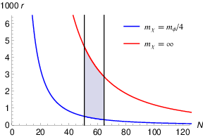
The bound (4.9) on is also a prediction of the theory, required by the consistency of the fakeon projection with inflationary cosmology. Because of it, the tensor-to-scalar ratio and the spectral index are predicted within less than one order of magnitude. Precisely,
| (7.5) |
For example, for we have
The allowed values of are shown in fig. 1, where the vertical lines denote the minimum and maximum values of in the range at 68% CL [21]. The windows (7.5) are compatible with the data available at present, which give [21].
The results of this paper also provide corrections to the amplitudes, which can be used to estimate the theoretical errors. From (7.2) we find
so we obtain
With , the first correction to is between 0.3% () and 2.5% (). Although and do not depend on in our approximation, they will at higher orders.
8 Conclusions
We have worked out the predictions of quantum gravity with fakeons on inflationary cosmology. By expanding around the de Sitter background the amplitudes and spectral indices of the scalar and tensor fluctuations have been calculated to the next-to-leading orders, comparing different frameworks, which lead to matching results. The physical content of the theory is exhausted by the two power spectra. The vector degrees of freedom, as well as the other scalar and tensor ones, are handled by means of the fakeon prescription and projected away. The methodologies we have developed to deal with this operation appear to be generalizable to higher orders.
The local, renormalizable, unitary, perturbative quantum field theory of gravity considered in this paper depends only on four parameters: the cosmological constant, Newton’s constant, and . The values of the cosmological constant and Newton’s constant are known. It will be possible to derive the values of and from and once new cosmological data will be available [39]. At that point, the theory will be uniquely determined and all other predictions (tensor tilt, running of the spectral indices, and so on) will be stringent tests of its validity.
The consistency of the approach puts a lower bound on the mass of the fakeon with respect to the mass of the scalar field. The tensor-to-scalar ratio is determined within less than an order of magnitude. Moreover, the relation is not affected by within our approximation. A separate analysis is required to study the case where the consistency bound on is violated and work out the consequences of the violation on the physics of the primordial universe. Finally, the investigation of this paper and the results we have obtained shed light on the problem of understanding purely virtual particles in curved space.
Acknowledgments
We are grateful to Denis Comelli and Gianfranco Cordella for helpful discussions. E.B. is supported by the NSF Grant No. PHY-1806428 and acknowledges the support of the ID 61466 Grant from the John Templeton Foundation (JTF), as part of the QISS project. M.P. is supported by the Estonian Research Council grants PRG803 and MOBTT86 and by the EU through the European Regional Development Fund CoE program TK133 “The Dark Side of the Universe”. M.P. is also grateful to Fondazione Angelo Della Riccia for financial support during the early stage of this work.
Appendices
A Map relating the inflaton framework to the geometric framework
In this appendix we derive some expansions used in the paper and show that the results of the inflaton and geometric frameworks agree with each other. For definiteness, the quantities with bars (, , , , , etc.) refer to the inflaton framework, while the quantities without bars (, , , , , etc.) refer to the geometric framework.
We start by determining in the geometric formalism. Writing the most general expansion
| (A.1) |
the numerical coefficients are calculated by differentiating (A.1) and then using the definition (3.5), the equation (5.1) and (A.1) again. This procedure gives an equality of two power series. Matching the coefficients recursively, we obtain for every . To the lowest orders, the result is
| (A.2) |
If we continue to arbitrary orders, we find an asymptotic series.
The action (2.4) is obtained from (2.1) by means of the conformal transformation (2.3). If we want to map the parametrizations (3.6) and (3.37) of the background metrics into each other, we need to combine that transformation with a time redefinition , so that
| (A.3) |
We split the conformal factor into the sum of its background part and the fluctuation . Using (5.10) and the second equation of (2.3), it is easy to find
| (A.4) |
The transformations of the background quantities are
| (A.5) |
plus those of and , which follow directly from their definitions. Using (5.1), (5.4) and (5.2), we find, to the lowest orders,
| (A.6) |
The relations can be extended to arbitrary orders, if needed. We find and d, which justifies the organization (3.3) of the expansion around the de Sitter background in the inflaton framework. In particular, inverting we get
| (A.7) | |||||
The last formula is derived from (A.2). Without passing through the geometric framework, the relations (A.7) can be worked out directly in the inflaton framework by expanding the equations (3.1) around the de Sitter background.
The map relating the fluctuations can be worked out from (A.3). The tensor modes and are clearly invariant,
| (A.8) |
while the scalar fluctuations and transform as
| (A.9) |
These formulas are written up to corrections of orders , , and , respectively. We can omit them for our purposes, since they do not affect the quadratic action and the two-point functions. We recall that the action is expanded around a solution of the equations of motion (which is then expanded around the de Sitter metric – which is not an exact solution), so the linear terms in the fluctuations are absent. Switching from one framework to the other, the corrections just mentioned affect the cubic terms, but not the quadratic ones.
From (A.9) we derive the transformation of the curvature perturbation . Observe that, given a scalar , where denotes the fluctuation around its background value , the combination
| (A.10) |
is invariant under infinitesimal time reparametrizations. If we choose and use the relations (A.4), we find, in the geometric framework,
| (A.11) |
the last equality following from (5.11). Using (A.4), (A.5) and (A.9) to rewrite this expression in the inflaton framework, we obtain
| (A.12) |
where is the background value of , such that . We recall that in section (3.2) the comoving gauge was used, so we just had there. Equations (A.11) and (A.12) prove that , so is also invariant when we switch frameworks.
This fact, together with (A.8), ensures that the power spectra calculated in the paper coincide in the two frameworks. We can use the formulas (A.6) to check it explicitly to the orders we have been working with. Comparing (3.36) with (5.8), (5.26) and (5.9), we find
Finally, comparing (3.46) and (3.47) with (5.18), (5.19) and (5.28), it is easy to verify that
B Superhorizon evolution
In this appendix we show that the curvature perturbation can be considered constant on superhorizon scales for adiabatic fluctuations of the energy-momentum tensor, in particular after the metric fluctuations exit the horizon and before they re-enter it. We start by showing this result in the inflaton framework.
Consider the energy momentum tensor with components
where , , and are its scalar fluctuations around the background. The gauge invariant curvature perturbation is
| (B.1) |
The unprojected equations derived from the action (2.4) for the metric (3.37) in the Newton gauge () read
| (B.2) |
where and the contributions of the scalar field are moved into . It is possible to show that formulas (B.2), together with the Friedmann equations
imply the equation
| (B.3) |
Thus, for adiabatic fluctuations
and on superhorizon scales , the scalar is practically constant. Since the property holds for the whole set of solutions of the unprojected equations, it also holds for the projected ones. Note that after the end of inflation is no longer small, so the factor in front in (B.3) is not a source of trouble.
In the geometric framework we reach the same conclusions. It is sufficient to work with the action (2.2) and note that the only difference with respect to the formulas just written is a redefinition of , brought by the variation of the terms containing with respect to the metric. Since we are considering only scalar quantities here, this is just a redefinition of , and the fluctuations , , and . Observe that we may need a nontrivial for this redefinition, which is the reason why we kept it nonzero in the derivation above.
References
- [1] R. Brout, F. Englert and E. Gunzig, The creation of the universe as a quantum phenomenon, Annals Phys. 115 (1978) 78.
- [2] A.A. Starobinsky, A new type of isotropic cosmological models without singularity, Phys. Lett. B 91 (1980) 99.
- [3] D. Kazanas, Dynamics of the universe and spontaneous symmetry breaking, Astrophys. J. 241 (1980) L59.
- [4] K. Sato, First-order phase transition of a vacuum and the expansion of the universe, Monthly Notices of the Royal Astr. Soc. 195 (1981) 467.
- [5] A.H. Guth, Inflationary universe: A possible solution to the horizon and flatness problems, Phys. Rev. D23 (1981) 347.
- [6] A.D. Linde, A new inflationary universe scenario: A possible solution of the horizon, flatness, homogeneity, isotropy and primordial monopole problems, Phys. Lett. B108 (1982) 389.
- [7] A. Albrecht and P.J. Steinhardt, Cosmology for grand unified theories with radiatively induced symmetry breaking, Phys. Rev. Lett. 48 (1982) 1220.
- [8] A.D. Linde, Chaotic inflation, Phys. Lett. B129 (1983) 177.
- [9] V.F. Mukhanov, G.V. Chibisov, Quantum fluctuations and a nonsingular universe, JETP Lett. 33 (1981) 532, Pisma Zh. Eksp. Teor. Fiz. 33 (1981) 549.
- [10] V.F. Mukhanov and G. Chibisov, The Vacuum energy and large scale structure of the universe, Sov. Phys. JETP 56 (1982) 258.
- [11] S. Hawking, The development of irregularities in a single bubble inflationary universe, Phys. Lett. B115 (1982) 295.
- [12] A.H. Guth and S. Pi, Fluctuations in the new inflationary universe, Phys. Rev. Lett. 49 (1982) 1110.
- [13] A.A. Starobinsky, Dynamics of phase transition in the new inflationary universe scenario and generation of perturbations, Phys. Lett. B117 (1982) 175.
- [14] J.M. Bardeen, P.J. Steinhardt and M.S. Turner, Spontaneous creation of almost scale-free density perturbations in an inflationary universe, Phys. Rev. D28 (1983) 679.
- [15] V.F. Mukhanov, Gravitational instability of the universe filled with a scalar field JETP Lett. 41 (1985) 493.
- [16] S. Weinberg, Cosmology, Oxford University Press, 2008.
- [17] V.F. Mukhanov, H.A. Feldman and R.H. Brandenberger, Phys. Rept. 215 (1992) 203; D. Baumann, TASI lectures on inflation, arXiv:0907.5424 [hep-th].
- [18] A. De Felice and S. Tsujikawa, theories, Living Rev. Rel. 13 (2010) 3 and arXiv:1002.4928 [gr-qc].
- [19] T.P. Sotiriou and V. Faraoni, theories of gravity, Rev. Mod. Phys. 82 (2010) 451 arXiv:0805.1726 [gr-qc].
- [20] J. Martin, C. Ringeval and V. Vennin, Encyclopaedia Inflationaris, Phys. Dark Univ. 5 (2014) 75 and arXiv:1303.3787 [astro-ph.CO]; J. Martin, C. Ringeval, R. Trotta and V. Vennin, The best inflationary models after Planck, JCAP 1403 (2014) 039 and arXiv:1312.3529 [astro-ph.CO].
- [21] Planck collaboration, Planck 2018 results. X. Constraints on inflation, arXiv:1807.06211 [astro-ph.CO].
- [22] S. Weinberg, Effective field theory for inflation, Phys. Rev. D 77 (2008) 123541 and arXiv:0804.4291 [hep-th].
- [23] S.W. Hawking and T. Hertog, Living with ghosts, Phys. Rev. D 6 (2002) 103515 and arXiv:hep-th/0107088.
- [24] D. Anselmi, On the quantum field theory of the gravitational interactions, J. High Energy Phys. 06 (2017) 086, 17A3 Renormalization.com and arXiv: 1704.07728 [hep-th].
- [25] D. Anselmi, Fakeons and Lee-Wick models, J. High Energy Phys. 02 (2018) 141, 18A1 Renormalization.com and arXiv:1801.00915 [hep-th].
- [26] D. Anselmi, The quest for purely virtual quanta: fakeons versus Feynman-Wheeler particles, J. High Energy Phys. 03 (2020) 142, 20A1 Renormalization.com and arXiv:2001.01942 [hep-th].
- [27] D. Anselmi and M. Piva, The ultraviolet behavior of quantum gravity, J. High Energ. Phys. 05 (2018) 27, 18A2 Renormalization.com and arXiv:1803.07777 [hep-th].
- [28] D. Anselmi and M. Piva, Quantum gravity, fakeons and microcausality, J. High Energy Phys. 11 (2018) 21, 18A3 Renormalization.com and arXiv:1806.03605 [hep-th].
- [29] S. Weinberg, Quantum contributions to cosmological correlations, Phys. Rev. D72 (2005) 043514 and arXiv:hep-th/0506236.
- [30] D. Anselmi, Fakeons, microcausality and the classical limit of quantum gravity, Class. and Quantum Grav. 36 (2019) 065010, 18A4 Renormalization.com and arXiv:1809.05037 [hep-th].
- [31] T. Clunan and M. Sasaki, Tensor ghosts in the inflationary cosmology, Class. Quant. Grav. 27 (2010) 165014 and arXiv:0907.3868 [hep-th]; N. Deruelle, M. Sasaki, Y. Sendouda and A. Youssef, Inflation with a Weyl term, or ghosts at work, JCAP 1103 (2011) 040 and arXiv:1012.5202 [gr-qc]; N. Deruelle, M. Sasaki, Y. Sendouda and A. Youssef, Lorentz-violating vs ghost gravitons: the example of Weyl gravity, J. High Energ. Phys. 2012 (2012) 9 and arXiv:1202.3131 [gr-qc]; Y.S. Myung and T. Moon, Primordial massive gravitational waves from Einstein-Chern-Simons-Weyl gravity, JCAP 08 (2014) 061 and arXiv:1406.4367 [gr-qc]; K. Kannike, G. Hütsi, L. Pizza, A. Racioppi, M. Raidal, A. Salvio and A. Strumia, Dynamically induced Planck scale and inflation, J. High Energy Phys. 05 (2015) 065 and arXiv:1502.01334 [astro-ph.CO].
- [32] M.M. Ivanov and A.A. Tokareva, Cosmology with a light ghost, JCAP 12 (2016) 018 and arXiv:1610.05330 [hep-th]; A. Salvio, Inflationary perturbations in no-scale theories, Eur. Phys. J. C77 (2017) 267 and arXiv:1703.08012 [astro-ph.CO].
- [33] A.S. Koshelev, L. Modesto, L. Rachwal and A.A. Starobinsky, Occurrence of exact inflation in non-local UV-complete gravity, J. High Energy Phys. 11 (2016) 1 and arXiv:1604.03127 [hep-th].
- [34] A.S. Koshelev, K.S. Kumar and A.A. Starobinsky, inflation to probe non-perturbative quantum gravity, J. High Energy Phys. 1803 (2018) 071 and arXiv:1711.08864 [hep-th]; A.S. Koshelev, K.S. Kumar, A. Mazumdar and A.A. Starobinsky, Non-Gaussianities and tensor-to-scalar ratio in non-local -like inflation, arXiv:2003.00629 [hep-th].
- [35] A. Vilenkin, Classical and quantum cosmology of the Starobinsky inflationary model, Phys. Rev. D 32 (1985) 2511.
- [36] K.S. Stelle, Renormalization of higher derivative quantum gravity, Phys. Rev. D 16 (1977) 953.
- [37] D. Anselmi, Fakeons and the classicization of quantum gravity: the FLRW metric, J. High Energy Phys. 04 (2019) 61, 19A1 Renormalization.com and arXiv:1901.09273 [gr-qc].
- [38] See for example, P. Peters and J.P. Uzan, Primordial cosmology, Oxford University Press, 2009.
- [39] K.N. Abazajian et al., CMB-S4 Science Book, First Edition, arXiv:1610.02743 [astro-ph.CO].