A machine learning route between band mapping and band structure
Electronic band structure (BS) and crystal structure are the two complementary identifiers of solid state materials. While convenient instruments and reconstruction algorithms have made large, empirical, crystal structure databases possible, extracting quasiparticle dispersion (closely related to BS) from photoemission band mapping data is currently limited by the available computational methods. To cope with the growing size and scale of photoemission data, we develop a pipeline including probabilistic machine learning and the associated data processing, optimization and evaluation methods for band structure reconstruction, leveraging theoretical calculations. The pipeline reconstructs all 14 valence bands of a semiconductor and shows excellent performance on benchmarks and other materials datasets. The reconstruction uncovers previously inaccessible momentum-space structural information on both global and local scales, while realizing a path towards integration with materials science databases. Our approach illustrates the potential of combining machine learning and domain knowledge for scalable feature extraction in multidimensional data.
Introduction
The modelling and characterization of the electronic BS of materials play an essential role in materials design [221] and device simulation [222]. The BS lives in the momentum space, and imprints the multidimensional and multi-valued functional relations between energy () and momenta () of periodically confined electrons [223]. Photoemission band mapping [224] (see Fig. 1a) using momentum- and energy-resolved photoemission spectroscopy (PES), including angle-resolved PES (ARPES) [225, 226] and multidimensional PES [227, 228] measures the BS as an intensity-valued multivariate probability distribution directly in . The proliferation of band mapping datasets and their public availability brought about by recent hardware upgrades [227, 228, 229, 230] have ushered in the possibilities of comprehensive benchmarking between theories and experiments, which become especially challenging for multiband materials with complex band dispersions [231, 232, 233]. The available methods for interpreting the photoemission spectra fall into two categories: Physics-based methods require least-squares fitting of 1D lineshapes, named energy or momentum distribution curves (EDCs or MDCs), to analytical models [234, 225, 235]. Although physics-informed data models guarantee high accuracy and interpretability, upscaling the pointwise fitting (or estimation) to large, densely sampled regions in the momentum space (e.g. including or more momentum locations) presents challenges due to limited numerical stability and efficiency. Therefore, their use is limited to selected momentum locations determined heuristically from physical knowledge of the materials and the experimental settings. Image processing-based methods apply data transformations to improve the visibility of dispersive features [236, 237, 238, 239]. They are more computationally efficient and can operate on entire datasets, yet offer only visual enhancement of the underlying band dispersion. They don’t allow reconstruction and therefore are insufficient for truly quantitative benchmarking or archiving.
A method balancing the two sides will extract the band dispersion with sufficiently high accuracy and be scalable to multidimensional datasets, therefore providing the basis for distilling structural information from complex band mapping data and for building efficient tools for annotating and understanding spectra. In this regard, we propose a computational framework (see Fig. 1b) for global reconstruction of the photoemission (or quasiparticle) BS as a set of energy (or electronic) bands, formed by energy values (i.e. band loci) connected along momentum coordinates. This local connectedness assumption is more valid than using local maxima of photoemission intensities because local maxima are not always good indicators of band loci [240]. We exploit the connection between theory and experiment in our framework, based on a probabilistic machine learning [241, 242] model to approximate the intensity data from band mapping experiments. The gist of the model is rooted in Bayes rule,
| (1) |
where are the random variables to be inferred and the data are mapped directly onto unknowns and experimental observables. We assign the energy values of the photoemission BS as the model’s variables to extract from data, and a nearest-neighbor (NN) Gaussian distribution as the prior, , to describe the proximity of energy values at nearby momenta. The EDC at every momentum grid point relates to the likelihood, , when we interpret the photoemission intensity probabilistically. The optimum is obtained via maximum a posteriori (MAP) estimation in probabilistic inference [241] (see Methods and Supplementary Fig. 2). Given the form of the NN prior, the posterior, , in the current setting forms a Markov random field (MRF) [241, 243, 244], which encapsulates the energy band continuity assumption and the measured intensity distribution of photoemission in a probabilistic graphical model. For one benefit, the probabilistic formulation can incorporate imperfect physical knowledge algebraically in the model or numerically as initialization (i.e. warm start, see Methods) of the MAP estimation, without requiring de facto ground truth and training as in supervised machine learning [245]. For another, the graphical model representation allows convenient optimization and extension to other dimensions (see Supplementary Fig. 1 and Section 1).

To demonstrate the effectiveness of the method, we have first reconstructed the entire 3D dispersion surfaces, , of all 14 valence bands within the projected first Brillouin zone (in (, , ) coordinates) of the semiconductor tungsten diselenide (WSe2), spanning 7 eV in energy and 3 along each momentum direction. Furthermore, we adapt informatics tools to BS data to sample and compare the reconstructed and theoretical BSs globally. The accuracy of the reconstruction is validated using synthetic data and the extracted local structural parameters in comparison with pointwise fitting. The available data and BS informatics enable detailed comparison of band dispersion at a resolution of 0.02 Å-1. Besides, we performed various tests and benchmarking on datasets of other materials and simulated data, where ground truth is available to evaluate the accuracy and computational efficiency.
Results
Band structure reconstruction and digitization. Our primary example is the 2D layered semiconductor WSe2 in the hexagonal lattice with a bilayer stacking periodicity (denoted as 2-WSe2) is a model system for band mapping experiments [247, 248, 231]. Earlier valence band mapping and reconstruction in ARPES experiments on WSe2 have demonstrated a high degree of similarity between theory and experiments [247, 248, 231], but a quantitative assessment within the entire (projected) Brillouin zone is still lacking. The valence BS of 2-WSe2 contains 14 strongly dispersive energy bands, formed by a mixture of the and orbitals of the W atoms and the orbitals of the Se atoms in its hexagonal unit cell. The strong spin-orbit coupling due to heavy elements produces large momentum- and spin-dependent energy splitting and modifications to the BS [231, 249].
We use a 2D MRF to model the loci of an energy band within the intensity-valued 3D band mapping data, regarded as a collection of momentum-ordered EDCs. It is graphically represented by a rectangular grid overlaid on the momentum axes with the indices (, are nonnegative integers), as shown in step (3) of Fig. 1b. The undetermined band energy of the EDC at , with the associated momentum coordinates , is considered a random variable, , of the MRF. Together, the probabilistic model is characterized by a joint distribution, expressed as the product of the likelihood and the Gaussian prior, in Eq. (1). To maintain its simplicity, we don’t explicitly account for the intensity modulations of various origins (such as imbalanced transition matrix elements [240]) in the original band mapping data, which cannot be remediated by upgrading the photon source or detector. Instead, we preprocess the data to minimize their effects on the reconstruction (see Fig. 1c-f). The preprocessing steps include (1) intensity symmetrization, (2) contrast enhancement [246], followed by (3) Gaussian smoothing (see Methods), whereafter the continuity of band-like features is restored. The EDCs from the preprocessed data, , are used effectively as the likelihood to calculate the MRF joint distribution,
| (2) |
Here, is a normalization constant, is a hyperparameter defining the width of the Gaussian prior, denotes the product over all discrete momentum values sampled in the experiment and the product over all the NN terms. A detailed derivation of Eq. (2) is given in Supplementary Section 1. Reconstruction of the bands in the photoemission BS is carried out sequentially and relies on local optimization of the MRF’s variables, .
To optimize over large graphical models, we adopt multiple parallelization schemes to achieve efficient operations on scalable computing hardware. A single band reconstruction involving optimization over random variables is achieved within seconds and hyperparameter tuning within tens of minutes (see Methods, Supplementary Figs. 3-4). In comparison, pointwise fitting often requires hand-tuning individually and therefore difficult to scale up to whole bands accordingly within a meaningful timeframe. To correctly resolve band crossings and nearly degenerate energies, we further inject relevant physical knowledge in the optimization by using density functional theory (DFT) band structure calculation with semi-local approximation [250] as a starting point for the reconstruction. The calculation qualitatively entails such physical symmetry information for WSe2, albeit not quantitatively reproducing the experimental quasiparticle BSs at all momentum coordinates. As shown with four DFT calculations with different exchange-correlation functionals [250] to initiate the reconstruction for WSe2 and in various cases using synthetic data with known ground truth (see Methods, Supplementary Table 3 and Supplementary Figs. 4-8), the reconstruction algorithm is not particularly sensitive to the initialization as long as the information about band crossings is present. The current framework can also support the initialization from more advanced electronic structure methods, such as [251] or that including electronic self-energies renormalized by electron-phonon coupling [252], when semi-local approximation yields not only quantitatively, but also qualitatively wrong quasiparticle BSs compared with the experiment. However, a systematic benchmark of theory and experiment goes beyond the scope of this work.

The reconstructed 14 valence bands of WSe2 initialized by LDA-level DFT are shown in Fig. 2b-d and Supplementary Videos. To globally compare the computed and reconstructed bands at a consistent resolution, we expand the BS in orthonormal polynomial bases [253], which are global shape descriptors and unbiased by the underlying electronic detail. The geometric featurization of band dispersion allows multiscale sampling and comparison using the coefficient (or feature) vectors [254]. We choose Zernike polynomials (ZPs) to decompose the 3D dispersion surfaces (see Fig. 3 and Methods) because of their existing adaptations to various boundary conditions [255].

In Fig. 3a-b, the band dispersions show generally decreasing dependence (seen from the magnitude of coefficients) on basis terms with increasing complexities (see Fig. 3a), and the majority of dispersion is encoded into a subset of the terms (see Fig. 3b). This observation implies that moderate smoothing may be applied to remove high-frequency features to improve the reconstruction in case of limited-quality data (acquired without sufficient accumulation time), which is often unavoidable when materials exhibit vacuum degradation, or during experimental parameter tuning. The example in Fig. 3b and additional numerical evidence in Supplementary Fig. 14 illustrate the approximation capability of the hexagonal ZPs. Concisely, these coefficients act as geometric fingerprints of the energy band dispersion, which enable the use of similarity or distance metrics (see Methods) for their comparison [254]. In Fig. 3c, the positive cosine similarity confirms the strong shape (or dispersion) resemblance of the 7 pairs of spin-split energy bands in the reconstructed BS of WSe2, while the low negative values, such as those between bands 1-2 and 13-14, reflect the opposite directions of their respective dispersion (see Fig. 2d). These observations are consistent with the outcome obtained from DFT calculations (see Supplementary Fig. 13).
Computational metrics and performance. To quantify the computational advantages of the machine learning-based reconstruction approach, we examine the outcome from diverse perspectives in consistency, accuracy and cost. To assess the consistency of reconstruction in its entirety, we introduce a BS distance metric (see Methods), invariant to the global energy shift frequently used to adjust the energy zero, to quantify the differences in band dispersion and the relative spacing between bands, which are the two major sources of variation between theories and experiments. The distance is calculated using the geometric fingerprints to bypass interpolation errors while reconciling the coordinate spacing difference between reconstructed and theoretical BSs, essential for differentiating BS data from heterogeneous sources in materials science databases [256, 257]. The results in Fig. 3d refer to the valence BS of WSe2 discussed in this work, where the distances and their spread (i.e. standard errors) are displayed in the upper and lower triangles, respectively. A high degree of consistency exists among the reconstructions (pairwise distance no larger than 608 meV/band) regardless of the level of DFT calculation used for initialization, indicating the robustness of the probabilistic reconstruction algorithm, whereas the distances between the DFT calculations are much larger, both in energy shifts and their spread. As shown in Fig. 3d and Supplementary Fig. 5, the learning algorithm can effectively reduce the epistemic uncertainty [258] between theories to obtain a consistent reconstruction.
To demonstrate the computational advantage of the MRF reconstruction over traditional line fitting methods, we benchmarked the outcome over selected regions in synthetic photoemission data. The regions are chosen based on their importance and we limit the size to have a manageable computing time (about an hour on our computing cluster at maximum for a single run), determined by the slower method, and allow for hyperparameter tuning, which requires tens of runs. The line fitting approach uses the Levenberg-Marquardt least squares optimization [260] with bound constraints for multicomponent photoemission spectra composed of a series of lineshape functions. We used the benchmark established in [259] for pointwise line fitting employing high-performance computing and two synthetic datasets with known ground truth dispersion, representing the local and global settings of the band structure reconstruction problem (see Supplementary Section 2.5). The synthetic data were based on band structure at the LDA-DFT level around the K point and along the high-symmetry line of the Brillouin zone. To level the hardware requirements, we used only distributed multicore-CPU computing for performance benchmarking. The estimated computing times are normalized to the per-band per-spectrum level [259]. The accuracy of the reconstruction is calculated using root-mean-squared (RMS) error, while the stability is quantified by the standard deviation of the residuals, which measures surface roughness [261]. The benchmarking results are compiled in Fig. 4 and Supplementary Table 2. They show that, compared with pointwise line fitting, the MRF reconstruction offers a considerable reduction in both normalized computing time and hyperparameter tuning time, while achieving consistently higher accuracy and stability in all but the two-band case. The combination of accuracy and stability in MRF reconstruction is due to the connectivity built into the prior, whereas in the pointwise fitting approach, information is not explicitly shared among neighbors. Since the number of bands reflects the complexity of multicomponent spectra, a near-constant normalized computing time and hyperparameter tuning time (see Fig. 4a-b) in MRF reconstruction regardless of the number of bands (or spectral components) allow us to scale up the computation to datasets comprising 104-105 or more spectra. The substantial gain in computational efficiency is a result of the inherent divide-and-conquer strategy in our BS reconstruction problem formulation and the associated distributed optimization method in the algorithm design. Comparatively, the distributed pointwise fitting exhibits a quasi-linear computational scaling with respect to the number of bands. When hyperparameter tuning is taken into account, in practice, it is only feasible for fitting small datasets with up to 103 multicomponent spectra [259].
Extended use cases and applications. The band dispersions recovered from photoemission data are often examined locally near dispersion extrema. We show in Fig. 5 that, besides providing global structural information, the reconstruction improves the robustness of traditional pointwise lineshape fitting in extended regions of the momentum space, when used as initial guess, because BS calculations may exhibit appreciable momentum-dependent deviations from experimental data that prevent them from being a sufficiently good starting point. Pointwise fitting in turn acts as the refinement of local details not explicitly included in the probabilistic reconstruction model, which prioritizes efficiency. This sequential approach recovers large regions in the Brillouin zone at high energy resolution without laborious hand-tuning of the fitting parameters per photoemission spectrum. Adopting this approach to WSe2, we recovered (i) a compendium of local band structure parameters (see Supplementary Table 4). The trigonal warping parameters of the first two valence bands around the -point are 5.8 eV and 3.9 eV, respectively, confirming the magnitude difference between these spin-split bands predicted by theory [249]. The warping signature extends further to high-energy bands. (ii) Dispersion fitting around the saddle point (and ) of the band structure reveals that the gap opened by spin-orbit interaction extends beyond it anisotropically on the dispersion surfaces with the minimum gap at 338 meV, markedly larger than DFT results, which predict degeneracy [249]. We expect this observation to contribute to the spin-dependent optical absorption due to the association of the saddle point in energy dispersion with a van Hove singularity [249, 262].

In addition to WSe2, we have performed BS reconstruction on two other photoemission datasets from other classes of materials: (1) Bismuth tellurium selenide (Bi2Te2Se), a topological insulator, measured using the same laboratory photoemission setup (see Fig. 6a-e) as for the WSe2 dataset. Although we used only simple numerical functions (Gaussian and paraboloid) to initialize the MRF reconstruction, the outcome demonstrates correct discrete momentum-space symmetry and details of energy dispersion down to the concave-shaped hexagonal warping in the band energy contours around the Dirac point [263]. Four energy bands, including the two low-energy valence bands, a surface-state energy band, and a partially occupied conduction band, were recovered using our approach for Bi2Te2Se. (2) Bulk gold (Au) photoemission dataset measured at a synchrotron X-ray source (see Fig. 6f-g). We used DFT calculations as the initialization to reconstruct four of the bulk energy bands, which are usually very challenging to extract by hand tracing or parametric function fitting, due in part to blurring ( dispersion) from the 3D characteristics of the electrons in the metallic bulk. Further discussions on these two materials and their band reconstructions are provided in Supplementary Section 3.

Discussion
The reconstruction approach described here provides a quantitative connection between empirical band dispersion () obtained from photoemission band mapping and their theoretical counterparts () through various orders of momentum-dependent “perturbations” (). The connection may be expressed as,
| (3) |
In Eq. (3), is the band index, represents electron self-energy, the zeroth-order term () means a rigid shift, while higher-order terms have increasing momentum-dependent nonlinearities. Our results here demonstrate that this formulation leads to practical band reconstruction, which recovers the accumulated “perturbations” () in Eq. (3) for every experimentally resolvable energy band. The outcome with current reconstruction accuracy and stability should assist interpretation of deep-lying bands, parametrizing multiband Hamiltonian models [264]. The data size reduction by over 5000 times from 3D band mapping data to geometric features vectors (see Methods) facilitates database integration [257, 265].
Apart from the benefits, we want to outline three limitations of our reconstruction approach. Firstly, the reconstruction approach doesn’t work ab initio and requires knowing the number of energy bands, , as implicated by the correspondence in Eq. (3). Although in simple datasets with up to several bands, can be estimated using prior knowledge of the material or from visual inspection, correctly estimating in complex datasets still requires calculated band structures. Secondly, when the electron self-energy modulation is significant, separating the so-called bare-band dispersion (i.e. single-particle dispersion) from the quasiparticle dispersion is needed for understanding the materials physics [266]. This requires re-evaluating the band structure reconstruction concept and consider the full spectral function (see Supplementary Section 1.1) explicitly to account for nonstandard lineshapes. Nevertheless, the outcome of our current approach may act as a trial solution for disentangling the bare-band dispersion relation from the electron self-energy [266]. Because the local connectedness assumption in Eq. (2) remains largely valid, our reconstruction may still recover the quasiparticle dispersion. We demonstrate this in Supplementary Fig. 10 using simulated photoemission data with a kink anomaly, a strong modification of dispersion from electron self-energy [225, 226]. Thirdly, an appropriate initialization may be expensive or impossible to obtain, either due to the computational cost, if higher-level theories (such as DFT with hybrid functionals and ) are required, or due to the complexity of the materials system, including undetermined microscopic interactions, sample defects or structural disorder, creating strong intensity blurring from dispersion, etc. These scenarios will remain challenging for band reconstruction.
Besides our demonstrations, we anticipate additional use cases that include (i) online monitoring [267] of band mapping experiments in the study of materials phase transitions [268] or functioning devices [269], where changes in atomic structure or carrier mobility are often accompanied by detectable changes in the electronic structure (including band dispersion), resulting in with time () dependence in addition to momentum () and energy. (ii) Spatial mapping of electronic structure variations for electronic devices via scanning photoemission measurements [270, 271], resulting in with spatial () dependence. In cases (i)-(ii), a fast reconstruction and evaluation framework may be used in a feedback loop to steer or optimize experimental conditions. (iii) Implementation of the reconstruction across various materials and to band-mapping data [227] conditioned on external parameters, including temperature, photon energy, dynamical time delay, and spin as resolved quantities, will generate comprehensive knowledge about the (non)equilibrium electronic structure of materials to benchmark theories. Moreover, the reconstruction method is (iv) transferable to extracting the band dispersion of other quasiparticles (e.g. phonons [272], polaritons [273], etc [274]) in periodic systems, given the availability of corresponding multidimensional datasets. (v) The analogy between band mapping and spatially-resolved spectral imaging, which produces location-dependent spectra, or suggests that the reconstruction algorithm may find use in teasing out the spatial (, ) variation of the spectral shifts, complementary to the outcome of clustering algorithms [275].
The increasing amount of publicly accessible and reusable datasets from materials science communities [265] motivate future extensions to the model with other types of informative priors that account for the full complexity of the physical signal while maintaining computational efficiency. Overall, the multidisciplinary methodology provides an example for building next-generation high-throughput materials characterization toolkits combining learning algorithms with physical knowledge [276] to arrive at a comprehensive understanding of materials properties unattainable before.
References
- [1] Eric. Isaacs and Chris Wolverton “Inverse Band Structure Design via Materials Database Screening: Application to Square Planar Thermoelectrics” In Chemistry of Materials 30.5, 2018, pp. 1540–1546 DOI: 10.1021/acs.chemmater.7b04496
- [2] E.. Marin et al. “Modeling of Electron Devices Based on 2-D Materials” In IEEE Transactions on Electron Devices 65.10, 2018, pp. 4167–4179 DOI: 10.1109/TED.2018.2854902
- [3] L.. Bouckaert, R. Smoluchowski and E. Wigner “Theory of Brillouin Zones and Symmetry Properties of Wave Functions in Crystals” In Physical Review 50.1, 1936, pp. 58–67 DOI: 10.1103/PhysRev.50.58
- [4] T.-C. Chiang and F. Seitz “Photoemission spectroscopy in solids” In Annalen der Physik 10.1-2, 2001, pp. 61–74 DOI: 10.1002/1521-3889(200102)10:1/2¡61::AID-ANDP61¿3.0.CO;2-G
- [5] Andrea Damascelli, Zahid Hussain and Zhi-Xun Shen “Angle-resolved photoemission studies of the cuprate superconductors” In Reviews of Modern Physics 75.2, 2003, pp. 473–541 DOI: 10.1103/RevModPhys.75.473
- [6] Hongyun Zhang et al. “Angle-resolved photoemission spectroscopy” In Nature Reviews Methods Primers 2.1, 2022, pp. 54 DOI: 10.1038/s43586-022-00133-7
- [7] Gerd Schönhense, Katerina Medjanik and Hans-Joachim Elmers “Space-, time- and spin-resolved photoemission” In Journal of Electron Spectroscopy and Related Phenomena 200, 2015, pp. 94–118 DOI: 10.1016/j.elspec.2015.05.016
- [8] K. Medjanik et al. “Direct 3D mapping of the Fermi surface and Fermi velocity” In Nature Materials 16.6, 2017, pp. 615–621 DOI: 10.1038/nmat4875
- [9] M. Puppin et al. “Time- and angle-resolved photoemission spectroscopy of solids in the extreme ultraviolet at 500 kHz repetition rate” In Review of Scientific Instruments 90.2, 2019, pp. 023104 DOI: 10.1063/1.5081938
- [10] Alexandre Gauthier et al. “Tuning time and energy resolution in time-resolved photoemission spectroscopy with nonlinear crystals” In Journal of Applied Physics 128.9, 2020, pp. 093101 DOI: 10.1063/5.0018834
- [11] J.. Riley et al. “Direct observation of spin-polarized bulk bands in an inversion-symmetric semiconductor” In Nature Physics 10.11, 2014, pp. 835–839 DOI: 10.1038/nphys3105
- [12] M.. Bahramy et al. “Ubiquitous formation of bulk Dirac cones and topological surface states from a single orbital manifold in transition-metal dichalcogenides” In Nature Materials 17.1, 2018, pp. 21–28 DOI: 10.1038/nmat5031
- [13] Niels.. Schröter et al. “Chiral topological semimetal with multifold band crossings and long Fermi arcs” In Nature Physics 15.8, 2019, pp. 759–765 DOI: 10.1038/s41567-019-0511-y
- [14] T. Valla et al. “Evidence for Quantum Critical Behavior in the Optimally Doped Cuprate Bi2Sr2CaCu2O8+δ” In Science 285.5436, 1999, pp. 2110–2113 DOI: 10.1126/science.285.5436.2110
- [15] G. Levy et al. “Deconstruction of resolution effects in angle-resolved photoemission” In Physical Review B 90.4, 2014, pp. 045150 DOI: 10.1103/PhysRevB.90.045150
- [16] P. Zhang et al. “A precise method for visualizing dispersive features in image plots” In Review of Scientific Instruments 82.4, 2011, pp. 043712 DOI: 10.1063/1.3585113
- [17] Yu He, Yan Wang and Zhi-Xun Shen “Visualizing dispersive features in 2D image via minimum gradient method” In Review of Scientific Instruments 88.7, 2017, pp. 073903 DOI: 10.1063/1.4993919
- [18] Han Peng et al. “Super resolution convolutional neural network for feature extraction in spectroscopic data” In Review of Scientific Instruments 91.3, 2020, pp. 033905 DOI: 10.1063/1.5132586
- [19] Younsik Kim et al. “Deep learning-based statistical noise reduction for multidimensional spectral data” In Review of Scientific Instruments 92.7, 2021, pp. 073901 DOI: 10.1063/5.0054920
- [20] Simon Moser “An experimentalist’s guide to the matrix element in angle resolved photoemission” In Journal of Electron Spectroscopy and Related Phenomena 214, 2017, pp. 29–52 DOI: 10.1016/j.elspec.2016.11.007
- [21] Kevin. Murphy “Machine Learning: A Probabilistic Perspective” MIT Press, 2012
- [22] Zoubin Ghahramani “Probabilistic machine learning and artificial intelligence” In Nature 521.7553, 2015, pp. 452–459 DOI: 10.1038/nature14541
- [23] Chaohui Wang, Nikos Komodakis and Nikos Paragios “Markov Random Field modeling, inference & learning in computer vision & image understanding: A survey” In Computer Vision and Image Understanding 117.11, 2013, pp. 1610–1627 DOI: https://doi.org/10.1016/j.cviu.2013.07.004
- [24] Mary Comer and Jeff Simmons “The Markov Random Field in Materials Applications: A synoptic view for signal processing and materials readers” In IEEE Signal Processing Magazine 39.1, 2022, pp. 16–24 DOI: 10.1109/MSP.2021.3123564
- [25] Kevin Kaufmann et al. “Crystal symmetry determination in electron diffraction using machine learning” In Science 367.6477, 2020, pp. 564–568 DOI: 10.1126/science.aay3062
- [26] Vincent Stimper et al. “Multidimensional Contrast Limited Adaptive Histogram Equalization” In IEEE Access 7, 2019, pp. 165437–165447 DOI: 10.1109/ACCESS.2019.2952899
- [27] M. Traving et al. “Electronic structure of WSe2: A combined photoemission and inverse photoemission study” In Physical Review B 55.16, 1997, pp. 10392–10399 DOI: 10.1103/PhysRevB.55.10392
- [28] Th. Finteis et al. “Occupied and unoccupied electronic band structure of WSe2” In Physical Review B 55.16, 1997, pp. 10400–10411 DOI: 10.1103/PhysRevB.55.10400
- [29] Andor Kormányos et al. “k · p theory for two-dimensional transition metal dichalcogenide semiconductors” In 2D Materials 2.2, 2015, pp. 022001 DOI: 10.1088/2053-1583/2/2/022001
- [30] John. Perdew and Karla Schmidt “Jacob’s ladder of density functional approximations for the exchange-correlation energy” In AIP Conference Proceedings 577 AIP, 2001, pp. 1–20 DOI: 10.1063/1.1390175
- [31] Dorothea Golze, Marc Dvorak and Patrick Rinke “The GW Compendium: A Practical Guide to Theoretical Photoemission Spectroscopy” In Frontiers in Chemistry 7:377, 2019 DOI: 10.3389/fchem.2019.00377
- [32] Marios Zacharias, Matthias Scheffler and Christian Carbogno “Fully anharmonic nonperturbative theory of vibronically renormalized electronic band structures” In Physical Review B 102.4, 2020, pp. 045126 DOI: 10.1103/PhysRevB.102.045126
- [33] Dengsheng Zhang and Guojun Lu “Review of shape representation and description techniques” In Pattern Recognition 37.1, 2004, pp. 1–19 DOI: 10.1016/j.patcog.2003.07.008
- [34] A. Khotanzad and Y.H. Hong “Invariant image recognition by Zernike moments” In IEEE Transactions on Pattern Analysis and Machine Intelligence 12.5, 1990, pp. 489–497 DOI: 10.1109/34.55109
- [35] Virendra. Mahajan and Guang-ming Dai “Orthonormal polynomials in wavefront analysis: analytical solution” In Journal of the Optical Society of America A 24.9, 2007, pp. 2994 DOI: 10.1364/JOSAA.24.002994
- [36] Lauri Himanen, Amber Geurts, Adam Foster and Patrick Rinke “Data‐Driven Materials Science: Status, Challenges, and Perspectives” In Advanced Science, 2019, pp. 1900808 DOI: 10.1002/advs.201900808
- [37] M.. Horton, S. Dwaraknath and K.. Persson “Promises and perils of computational materials databases” In Nature Computational Science 1.1, 2021, pp. 3–5 DOI: 10.1038/s43588-020-00016-5
- [38] Armen Kiureghian and Ove Ditlevsen “Aleatory or epistemic? Does it matter?” In Structural Safety 31.2, 2009, pp. 105–112 DOI: 10.1016/j.strusafe.2008.06.020
- [39] Rui Xian, Ralph Ernstorfer and Philipp Pelz “Scalable multicomponent spectral analysis for high-throughput data annotation” In arXiv, 2021, pp. 2102.05604 arXiv: http://arxiv.org/abs/2102.05604
- [40] Jorge Nocedal and Stephen. Wright “Numerical Optimization” Springer New York, 2006 DOI: 10.1007/978-0-387-40065-5
- [41] Mark. Smith “Roughness in the Earth Sciences” In Earth-Science Reviews 136, 2014, pp. 202–225 DOI: 10.1016/j.earscirev.2014.05.016
- [42] Huaihong Guo et al. “Double resonance Raman modes in monolayer and few-layer MoTe2” In Physical Review B 91.20, 2015, pp. 205415 DOI: 10.1103/PhysRevB.91.205415
- [43] Joseph. Heremans, Robert. Cava and Nitin Samarth “Tetradymites as thermoelectrics and topological insulators” In Nature Reviews Materials 2.10, 2017, pp. 17049 DOI: 10.1038/natrevmats.2017.49
- [44] “Multi-Band Effective Mass Approximations” 94, Lecture Notes in Computational Science and Engineering Springer, 2014 DOI: 10.1007/978-3-319-01427-2
- [45] Matthias Scheffler et al. “FAIR data enabling new horizons for materials research” In Nature 604.7907, 2022, pp. 635–642 DOI: 10.1038/s41586-022-04501-x
- [46] A.. Kordyuk et al. “Bare electron dispersion from experiment: Self-consistent self-energy analysis of photoemission data” In Physical Review B 71.21, 2005, pp. 214513 DOI: 10.1103/PhysRevB.71.214513
- [47] Marcus. Noack et al. “Gaussian processes for autonomous data acquisition at large-scale synchrotron and neutron facilities” In Nature Reviews Physics 3.10, 2021, pp. 685–697 DOI: 10.1038/s42254-021-00345-y
- [48] Samuel Beaulieu et al. “Ultrafast dynamical Lifshitz transition” In Science Advances 7.17, 2021, pp. eabd9275 DOI: 10.1126/sciadv.abd9275
- [49] Davide Curcio et al. “Accessing the Spectral Function in a Current-Carrying Device” In Physical Review Letters 125.23, 2020, pp. 236403 DOI: 10.1103/PhysRevLett.125.236403
- [50] Neil. Wilson et al. “Determination of band offsets, hybridization, and exciton binding in 2D semiconductor heterostructures” In Science Advances 3.2, 2017, pp. e1601832 DOI: 10.1126/sciadv.1601832
- [51] Søren Ulstrup et al. “Nanoscale mapping of quasiparticle band alignment” In Nature Communications 10.1, 2019, pp. 3283 DOI: 10.1038/s41467-019-11253-2
- [52] R.A. Ewings et al. “Horace : Software for the analysis of data from single crystal spectroscopy experiments at time-of-flight neutron instruments” In Nuclear Instruments and Methods in Physics Research Section A: Accelerators, Spectrometers, Detectors and Associated Equipment 834, 2016, pp. 132–142 DOI: 10.1016/j.nima.2016.07.036
- [53] C.. Whittaker et al. “Exciton Polaritons in a Two-Dimensional Lieb Lattice with Spin-Orbit Coupling” In Physical Review Letters 120.9, 2018, pp. 097401 DOI: 10.1103/PhysRevLett.120.097401
- [54] Andreas Frölich et al. “Frequency-Resolved Reciprocal-Space Mapping of Visible Spontaneous Emission from 3D Photonic Crystals” In Advanced Optical Materials 2.9, 2014, pp. 849–853 DOI: 10.1002/adom.201400150
- [55] Iban Amenabar et al. “Hyperspectral infrared nanoimaging of organic samples based on Fourier transform infrared nanospectroscopy” In Nature Communications 8.1, 2017, pp. 14402 DOI: 10.1038/ncomms14402
- [56] Laura von Rueden et al. “Informed Machine Learning - A Taxonomy and Survey of Integrating Prior Knowledge into Learning Systems” In IEEE Transactions on Knowledge and Data Engineering, 2021, pp. 1–1 DOI: 10.1109/TKDE.2021.3079836
- [57] A. Oelsner et al. “Microspectroscopy and imaging using a delay line detector in time-of-flight photoemission microscopy” In Review of Scientific Instruments 72.10, 2001, pp. 3968–3974 DOI: 10.1063/1.1405781
- [58] R. Xian et al. “An open-source, end-to-end workflow for multidimensional photoemission spectroscopy” In Scientific Data 7.1, 2020, pp. 442 DOI: 10.1038/s41597-020-00769-8
- [59] SPECS GmbH “METIS 1000 Brochure”, https://www.specs-group.com/fileadmin/user_upload/products/brochures/SPECS_Brochure-METIS_RZ_web.pdf, 2019
- [60] Rui Xian, Laurenz Rettig and Ralph Ernstorfer “Symmetry-guided nonrigid registration: The case for distortion correction in multidimensional photoemission spectroscopy” In Ultramicroscopy 202, 2019, pp. 133–139 DOI: 10.1016/j.ultramic.2019.04.004
- [61] J Kittler and J Föglein “Contextual classification of multispectral pixel data” In Image and Vision Computing 2.1, 1984, pp. 13–29 DOI: https://doi.org/10.1016/0262-8856(84)90040-4
- [62] Martín Abadi et al. “TensorFlow: Large-Scale Machine Learning on Heterogeneous Distributed Systems” In arXiv, 2016, pp. 1603.04467v2 arXiv: http://arxiv.org/abs/1603.04467
- [63] Stan Li “Markov Random Field Modeling in Image Analysis”, Advances in Pattern Recognition Springer, 2009
- [64] Vincent Stimper and Rui Xian “fuller”, https://github.com/mpes-kit/fuller URL: https://github.com/mpes-kit/fuller
- [65] Yoyo Hinuma et al. “Band structure diagram paths based on crystallography” In Computational Materials Science 128, 2017, pp. 140–184 DOI: 10.1016/j.commatsci.2016.10.015
- [66] D.. Ceperley and B.. Alder “Ground State of the Electron Gas by a Stochastic Method” In Physical Review Letters 45.7, 1980, pp. 566–569 DOI: 10.1103/PhysRevLett.45.566
- [67] John. Perdew and Yue Wang “Accurate and simple analytic representation of the electron-gas correlation energy” In Physical Review B 45.23, 1992, pp. 13244–13249 DOI: 10.1103/PhysRevB.45.13244
- [68] John. Perdew, Kieron Burke and Matthias Ernzerhof “Generalized Gradient Approximation Made Simple” In Physical Review Letters 77.18, 1996, pp. 3865–3868 DOI: 10.1103/PhysRevLett.77.3865
- [69] John. Perdew et al. “Restoring the Density-Gradient Expansion for Exchange in Solids and Surfaces” In Physical Review Letters 100.13, 2008, pp. 136406 DOI: 10.1103/PhysRevLett.100.136406
- [70] Jochen Heyd, Gustavo. Scuseria and Matthias Ernzerhof “Hybrid functionals based on a screened Coulomb potential” In The Journal of Chemical Physics 118.18, 2003, pp. 8207–8215 DOI: 10.1063/1.1564060
- [71] Volker Blum et al. “Ab initio molecular simulations with numeric atom-centered orbitals” In Computer Physics Communications 180.11, 2009, pp. 2175–2196 DOI: 10.1016/j.cpc.2009.06.022
- [72] William. Huhn and Volker Blum “One-hundred-three compound band-structure benchmark of post-self-consistent spin-orbit coupling treatments in density functional theory” In Physical Review Materials 1.3, 2017, pp. 033803 DOI: 10.1103/PhysRevMaterials.1.033803
- [73] James. Wyant and Katherine Creath “Basic wavefront aberration theory” In Applied Optics and Optical Engineering Xl Academic Press, 1992, pp. 1–53
- [74] David. Watkins “Fundamentals of matrix computations” Wiley, 2010
- [75] Stefan Hüfner “Photoelectron Spectroscopy”, Advanced Texts in Physics Springer Berlin Heidelberg, 2003 DOI: 10.1007/978-3-662-09280-4
- [76] Christopher. Bishop “Pattern Recognition and Machine Learning” Springer, 2006
- [77] J.. Hammersley and P. Clifford “Markov Fields on Finite Graphs and Lattices” Unpublished, 1971 URL: http://www.statslab.cam.ac.uk/~grg/books/hammfest/hamm-cliff.pdf
- [78] Julian Besag “Spatial Interaction and the Statistical Analysis of Lattice Systems” In Journal of the Royal Statistical Society. Series B (Methodological) 36.2 [Royal Statistical Society, Wiley], 1974, pp. 192–236 URL: http://www.jstor.org/stable/2984812
- [79] Stuart Geman and Donald Geman “Stochastic Relaxation, Gibbs Distributions, and the Bayesian Restoration of Images” In IEEE Transactions on Pattern Analysis and Machine Intelligence 6.6, 1984, pp. 721–741 DOI: 10.1109/TPAMI.1984.4767596
- [80] Julian Besag “On the Statistical Analysis of Dirty Pictures” In Journal of the Royal Statistical Society: Series B (Methodological) 48.3, 1986, pp. 259–279 DOI: 10.1111/j.2517-6161.1986.tb01412.x
- [81] Judea Pearl “Probabilistic Reasoning in Intelligent Systems” Morgan Kaufmann, 1988 DOI: 10.1016/C2009-0-27609-4
- [82] J. Besag “On the statistical analysis of nearest-neighbours” In Proceedings of the European Meeting of Statisticians, Budapest, 1972
- [83] M. Locatelli “A note on the Griewank test function” In Journal of Global Optimization 25.2, 2003, pp. 169–174 DOI: 10.1023/A:1021956306041
- [84] Cristina Bena and Gilles Montambaux “Remarks on the tight-binding model of graphene” In New Journal of Physics 11.9, 2009, pp. 095003 DOI: 10.1088/1367-2630/11/9/095003
- [85] Virendra. Mahajan and Guang-ming Dai “Orthonormal polynomials for hexagonal pupils” In Optics Letters 31.16, 2006, pp. 2462 DOI: 10.1364/OL.31.002462
- [86] H.. van Hulst and J… Reesinck “Line Breadths and Voigt Profiles.” In The Astrophysical Journal 106, 1947, pp. 121 DOI: 10.1086/144944
- [87] Mofreh. Zaghloul and Ahmed. Ali “Algorithm 916: Computing the Faddeyeva and Voigt Functions” In ACM Transactions on Mathematical Software 38.2, 2011, pp. 1–22 DOI: 10.1145/2049673.2049679
- [88] Shuo Dong et al. “Direct measurement of key exciton properties: Energy, dynamics, and spatial distribution of the wave function” In Natural Sciences 1.1, 2021, pp. 1:e10010 DOI: 10.1002/ntls.10010
- [89] S. LaShell, B.. McDougall and E. Jensen “Spin Splitting of an Au(111) Surface State Band Observed with Angle Resolved Photoelectron Spectroscopy” In Physical Review Letters 77.16, 1996, pp. 3419–3422 DOI: 10.1103/PhysRevLett.77.3419
- [90] Rui Xian “pesarxiv”, https://github.com/mpes-kit/pesarxiv URL: https://github.com/mpes-kit/pesarxiv
- [91] Carlos Grohmann, Mike. Smith and Claudio Riccomini “Multiscale Analysis of Topographic Surface Roughness in the Midland Valley, Scotland” In IEEE Transactions on Geoscience and Remote Sensing 49.4, 2011, pp. 1200–1213 DOI: 10.1109/TGRS.2010.2053546
- [92] Feliciano Giustino, Marvin. Cohen and Steven. Louie “Small phonon contribution to the photoemission kink in the copper oxide superconductors” In Nature 452.7190, 2008, pp. 975–978 DOI: 10.1038/nature06874
- [93] Carla Verdi, Fabio Caruso and Feliciano Giustino “Origin of the crossover from polarons to Fermi liquids in transition metal oxides” In Nature Communications 8.1, 2017, pp. 15769 DOI: 10.1038/ncomms15769
- [94] Jian-Li Mi et al. “Phase Separation and Bulk p-n Transition in Single Crystals of Bi2Te2Se Topological Insulator” In Advanced Materials 25.6, 2013, pp. 889–893 DOI: 10.1002/adma.201203542
- [95] Matteo Michiardi et al. “Strongly anisotropic spin-orbit splitting in a two-dimensional electron gas” In Physical Review B 91.3, 2015, pp. 035445 DOI: 10.1103/PhysRevB.91.035445
- [96] Antonin Chambolle “An Algorithm for Total Variation Minimization and Applications” In Journal of Mathematical Imaging and Vision 20.1-2 Springer, 2004, pp. 89–97 DOI: 10.1023/B:JMIV.0000011325.36760.1E
- [97] Stéfan van Walt et al. “scikit-image: image processing in Python” In PeerJ 2, 2014, pp. e453 DOI: 10.7717/peerj.453
- [98] E. Papalazarou et al. “Unraveling the Dirac fermion dynamics of the bulk-insulating topological system Bi2Te2Se” In Physical Review Materials 2.10, 2018, pp. 104202 DOI: 10.1103/PhysRevMaterials.2.104202
- [99] S.V. Hoffmann et al. “An undulator-based spherical grating monochromator beamline for angle-resolved photoemission spectroscopy” In Nuclear Instruments and Methods in Physics Research Section A: Accelerators, Spectrometers, Detectors and Associated Equipment 523.3, 2004, pp. 441–453 DOI: 10.1016/j.nima.2004.01.039
- [100] Maciej Dendzik et al. “Reconstruction-induced trefoil knot Fermi contour of Au(111)” In Physical Review B 94.20, 2016, pp. 201401 DOI: 10.1103/PhysRevB.94.201401
- [101] Christian Tusche, Alexander Krasyuk and Jürgen Kirschner “Spin resolved bandstructure imaging with a high resolution momentum microscope” In Ultramicroscopy 159, 2015, pp. 520–529 DOI: 10.1016/j.ultramic.2015.03.020
- [102] In-Bai Lin, Tony-Hann Sheu and Jia-Han Li “Effects of exchange correlation functional on optical permittivity of gold and electromagnetic responses” In Optics Express 22.25, 2014, pp. 30725 DOI: 10.1364/OE.22.030725
- [103] L. Ortenzi, E. Cappelluti, L. Benfatto and L. Pietronero “Fermi-Surface Shrinking and Interband Coupling in Iron-Based Pnictides” In Physical Review Letters 103.4, 2009, pp. 046404 DOI: 10.1103/PhysRevLett.103.046404
- [104] Junren Shi et al. “Direct Extraction of the Eliashberg Function for Electron-Phonon Coupling: A Case Study of Be(100)” In Physical Review Letters 92.18, 2004, pp. 186401 DOI: 10.1103/PhysRevLett.92.186401
- [105] P.. Allen and R.. Dynes “Transition temperature of strong-coupled superconductors reanalyzed” In Physical Review B 12.3, 1975, pp. 905–922 DOI: 10.1103/PhysRevB.12.905
- [106] Franz Knuth et al. “All-electron formalism for total energy strain derivatives and stress tensor components for numeric atom-centered orbitals” In Computer Physics Communications 190, 2015, pp. 33–50 DOI: https://doi.org/10.1016/j.cpc.2015.01.003
- [107] D. Voß, P. Krüger, A. Mazur and J. Pollmann “Atomic and electronic structure of WSe2 from ab initio theory: Bulk crystal and thin film systems” In Phys. Rev. B 60 American Physical Society, 1999, pp. 14311–14317 DOI: 10.1103/PhysRevB.60.14311
- [108] K Kam, C Chang and D Lynch “Fundamental absorption edges and indirect band gaps in WMoSe2 (01)” In Journal of Physics C: Solid State Physics 17.22 IOP Publishing, 1984, pp. 4031–4040 DOI: 10.1088/0022-3719/17/22/021
- [109] Sujay. Desai et al. “Strain-Induced Indirect to Direct Bandgap Transition in Multilayer WSe2” In Nano Letters 14.8, 2014, pp. 4592–4597 DOI: 10.1021/nl501638a
- [110] Matt Newville et al. “lmfit/lmfit-py 1.0.0” In Zenodo, https://doi.org/10.5281/zenodo.3588521, 2019 DOI: 10.5281/ZENODO.3588521
Methods
-
Band mapping measurements of WSe2. Multidimensional photoemission spectroscopy experiments were conducted with a laser-driven, high harmonic generation-based extreme UV light source [229] operating at 21.7 eV and 500 kHz and a METIS 1000 (SPECS GmbH) momentum microscope featuring a delay-line detector coupled to a time-of-flight drift tube [228, 277]. The experiment captures photoelectrons directly in their 3D coordinates, [227, 228]. Single crystal samples of WSe2 ( 99.995% pure) were purchased from HQ graphene and were used directly for measurements without further purification. Before measurements, the WSe2 samples were attached to the Cu substrate by conductive epoxy resin (EPO-TEK H20E). The samples were cleaved by cleaving pins attached to the sample surface upon transfer into the measurement chamber, which operates at an ambient pressure of mbar during photoemission experiments. No effect of surface termination has been observed in the measured WSe2 photoemission spectra, similar to previous experimental observations [247, 231]. For the valence band mapping experiments, the energy focal plane of the photoelectrons within the time-of-flight drift tube was set close to the top valence band. Although effects of sample degradation has also been reported [248] during the course of long-duration angular scanning in ARPES measurements, with our high-repetition-rate photon source [229] and the fast electronics of the momentum microscope, band mapping of WSe2 achieves sufficient signal-to-noise ratio for valence band reconstruction within only tens of minutes of data acquisition, without the need for angular scanning and subsequent reconstruction from momentum-space slices.
-
Data processing and reconstruction. The raw data, in the form of single-electron events recorded by the delay-line detector, were preprocessed using home-developed software packages [278]. The events were first binned to the grid with a size of 256256470 to cover the full valence band range in WSe2 within the projected Brillouin zone, which amounts to a pixel size of 0.015 along the momentum axes and 18 meV along the energy axis. The bin sizes are within the limits of the momentum resolution ( 0.01 ) and energy resolution ( 15 meV) of the photoelectron spectrometer [279].
Data binning is carried out in conjunction with the necessary lens distortion correction [280] and calibrations as described in [278]. The outcome provides a sufficient level of granularity in the momentum space to resolve the fine features in band dispersion while achieving higher signal-to-noise ratio than using single-event data directly. Afterwards, we applied intensity symmetrization to the data along the sixfold rotation symmetry and mirror symmetry axes [231] of the photoemission intensity pattern in the coordinates, followed by contrast enhancement using the multidimensional extension of the contrast limited adaptive histogram equalization (MCLAHE) algorithm, where the intensities in the image are transformed by a look-up table built from the normalized cumulative distribution function of local image patches [246]. Finally, we applied Gaussian smoothing to the data along the , and axes with a standard deviation of 0.8, 0.8 and 1 pixels (or about 0.012 , 0.012 , and 18 meV), respectively.
After data preprocessing, we sequentially reconstructed every energy band of WSe2 from the photoemission data using the maximum a posteriori (MAP) approach described in the main text. The reconstruction requires tuning of three hyperparameters: (1) the momentum scaling and (2) the rigid energy shift to coarse-align the computed energy band, e.g. from density functional theory (DFT), to the photoemission data, and (3) the width of the nearest-neighbor Gaussian prior ( in Eq. (2)). The hyperparameter tuning is also carried out individually for each band to adapt to their specific environment. An example of hyperparameter tuning is given in Supplementary Fig. 4. The MAP reconstruction method involves optimization of the band energy random variables, to maximize the posterior probability or to minimize the negative log-probability loss function, , obtained from Eq. (2) as is used in our actual implementation.
(4) We implemented the optimization using a parallelized version of the iterated conditional mode (ICM) [281] method in Tensorflow [282] in order to run on multicore computing clusters and GPUs. The parallelization involves a checkerboard coloring scheme (or coding method) of the graph nodes [283] and subsequent hierarchical grouping of colored nodes, which allows alternating updates on different subgraphs (i.e. subsets of the nodes) of the Markov random field during optimization. Typically, the optimization process in the reconstruction of one band converges within and therefore is terminated after 100 epochs, which takes 7 seconds on a single NVIDIA GTX980 GPU for the above-mentioned data size. Details on the parallelized implementation are provided in Supplementary Section 1. In addition, because symmetry information is not explicitly included in the MRF model, the reconstructed bands generally requires further symmetrization as refinement or post-processing to be ready for database integration.
We described our approach of using band structure calculations to initialize the MAP optimization as a warm start. The term ”warm start” in the context of numerical optimization generally refers to the initialization of an optimization using the outcome of an associated and yet more solvable problem (e.g. surrogate model) obtained beforehand that yields an approximate answer, instead of starting from scratch (i.e. cold start). Warm-starting an optimization improves the effective use of prior knowledge and its convergence rate [260]. In the current context, we regard the band structure reconstruction from photoemission band mapping data as the optimization problem to warm start, and the outcome from an electronic structure calculation can produce a sufficiently good approximate to the solution of the optimization problem. For WSe2, straightforward DFT calculations with semi-local approximation (which in itself involves explicit optimizations such as geometric optimization of the crystal structures) are sufficient, but our approach is not limited to DFT. Therefore, the use of ”warm start” in our application is conceptually well-aligned with the origin of the term.
To validate the MAP reconstruction algorithm in a variety of scenarios, we used synthetic photoemission data where the nominal ground-truth band structures are available. The band structures are constructed using analytic functions, model Hamiltonians or DFT calculations. The initializations are generated by tuning the numerical parameters used to generate the ground-truth band structures. The procedures and results are presented in Supplementary Section 2. In simple cases, such as single or well-isolated bands, the reconstruction yields a close solution to the ground truth even with a flat band initialization. In the more general multiband scenario with congested bands and band crossings (or anti-crossings), an approximate dispersion (or shape) of the band and the crossing information is required in the initialization (i.e. warm start) in order to converge to a realistic solution. We further tested the robustness of the initializations by (1) scaling the energies of the ground truth and by (2) using DFT calculations with different exchange-correlation (XC) functionals, in order to capture sufficient variability of available band structure calculations in the real world. We quantify the variations in the initializations and the performance of the reconstruction using the average error (Eq. (9), or Fig. 3b), calculated with respect to the ground truth. Among the different numerical experiments, we find that the optimization converges consistently to a set of bands that better matches the experimental data than the initialization. This is manifest in that the average errors of the initializations are reduced to a similar level in the corresponding reconstruction outcomes, a trend seen over all bands regardless of their dispersion. In the synthetic data with an energy spacing of 18 meV, the average error in the reconstruction is on the order of 40-50 meV for each band, which amounts to an average inaccuracy of 3 bins along the energy dimension at a momentum location. The inaccuracy is, however, dependent on the bin sizes used in the preprocessing and the fundamental resolution in the experiment. We have made the code for the MAP reconstruction algorithm and the synthetic data generation publicly accessible from the online repository fuller [284] for broader applications.
-
Visualization strategies. Band mapping and band structure data contain unique multidimensional data structures in materials science that are often presented with specific visualizations motivated by the underlying solid state physics and symmetry properties. In this work, we select a fixed set of 2D and 3D visualization techniques to illustrate their link and allow comparison with other photoemission studies of the same materials. Typically, ARPES data [226] of the form are sampled and visualized along a particular path (i.e. k-path [285]) in the momentum space [248, 247] where only specific high-symmetry positions are labeled with capital letters [223]. A canonical k-path exists for each symmetry setting [285]. Photoemission band mapping generates datasets with a dimensionality of three or higher and often contains a lower symmetry (in intensity ) as a result of the photoemission matrix elements [240] and the experimental condition. These factors lead to more flexibility in data representation [278] and motivate the use of alternative k-paths that capture the complexity of the photoemission spectra. In Fig. 1c-f for WSe2 and Fig. 6a-c for Bi2Te2Se, we combine 3D volumetric rendering and 2D k-path views to illustrate both the data symmetry and the intensity modulations present in the data.
To visualize band dispersion surfaces, , we combine 3D stacked surfaces and 2D image sequences, as exemplified in Fig. 2b, d for WSe2 and Fig. 6d, e for Bi2Te2Se. This paired approach balances the strengths and shortcomings of different viewpoints to achieve a comprehensive representation of the data type. The 3D stacked surface representation highlights the entirety and complexity of the data, but often contains occluded regions imperceptible from a fixed viewing direction. The 2D image sequence representation includes all energy dispersion information, yet loses the interrelationship on the energy scale between energy bands, which matter in the event of (anti)crossings. In combining these two approaches, we typically choose the same color map and scale to maintain referenceability between the two representations. For each energy band, the full color scale is used to cover its energy range, becoming the normalized energy scale, which illustrates the local detail of the dispersion that otherwise may be hard to discern.
-
Band structure calculations. Electronic band structures were calculated within (generalized) DFT using the local density approximation (LDA) [286, 287], the generalized-gradient approximation (GGA-PBE) [288] and GGA-PBEsol [289]), and the hybrid XC functional HSE06 [290], which incorporates a fraction of the exact exchange. All calculations were performed with the all-electron, full-potential numeric-atomic orbital code, FHI-aims [291]. They were conducted for the geometries obtained by fully relaxing the atomic structure with the respective XC-functional to keep the electronic and atomic structures consistent. Spin-orbit coupling was included in a perturbational fashion [292]. The momentum grid used for the calculation was equally sampled with a spacing of 0.012 in both and directions that covers the irreducible part of the first Brillouin zone at = 0.35 , estimated using the inner potential of WSe2 from a previous measurement [231]. The calculated band structure is symmetrized to fill the entire hexagonal Brillouin zone to be used to initialize the band structure reconstruction and synthetic data generation. We note here that for the MAP reconstruction, the momentum grid size used in theoretical calculations (such as DFT at various levels used here) need not be identical to that of the data (or instrument resolution) and in those cases an appropriate upsampling (or downsampling) should be applied to the calculation to match their momentum resolution. Further details are presented in Supplementary Section 4.
-
Band structure informatics. The shape feature space representation of each electronic band is derived from the decomposition,
(5) Here, represents the momentum coordinate, is the single-band dispersion relation (e.g. dispersion surface in 3D), and are the coefficient and its associated basis term, respectively. They are grouped separately into the feature vector, , and the basis vector, . The orthonormality of the basis is guaranteed within the projected Brillouin zone (PBZ) of the material.
(6) For the hexagonal PBZ of WSe2, the basis terms are hexagonal Zernike polynomials (ZPs) constructed using a linear combination of the circular ZPs via Gram-Schmidt orthonormalization within a regular (i.e. equilateral and equiangular) hexagon [255]. A similar method can be used to generate ZP-derived orthonormal basis adapted to other boundary conditions [255]. The representation in feature space [254] provides a way to quantify the difference (or distance) between energy bands or band structures at different resolutions or scales without additional interpolation. To quantify the shape similarity between energy bands and , we calculate the cosine similarity using the feature vectors,
(7) The cosine similarity is bounded within , with a value of 0 describing orthogonality of the feature vectors and a value of 1 and -1 describing parallel and anti-parallel relations between them, respectively, both indicating high similarity. The use of cosine similarity in feature space allows comparison of dispersion while being unaffected by their magnitudes. In comparing the dispersion between single energy bands using Eq. (7), the first term in the polynomial expansion, or the hexagonal equivalent of the Zernike piston [293], is discarded as it only represents a constant energy offset (with zero spatial frequency) instead of dispersion, which is characterized by a combination of finite and nonzero spatial frequencies.
The electronic band structure is a collection of energy bands . To quantify the distance between two band structures, and , containing the same number of energy bands while ignoring their global energy difference, we first subtract the energy grand mean (i.e. mean of the energy means of all bands within the region of the band structure for comparison). Then, we compute the Euclidean distance, or the -norm, for the th pair of bands, .
(8) Here, denotes the feature vector after subtracting the energy grand mean so that any global energy shift is removed. We define the band structure distance as the average distance over all pairs of bands, or = . The values of are shown in the upper triangle of Fig. 3d and their corresponding standard errors (over the 14 valence bands of WSe2) in the lower triangle. The distance in Eq. (8) is independent of basis and allows energy bands calculated on different resolutions or from different materials with the same symmetry (e.g. differing only by Brillouin zone size) to be compared.
We use same-resolution error metrics to evaluate the approximation quality of the expansion basis and to quantify the reconstruction outcome with a known ground-truth band structure. Specifically, we define the average approximation error (with energy unit), , for each energy band using the energy difference at every momentum location,
(9) where is the number of momentum grid points and the summation runs over the projected Brillouin zone. In addition, we construct the relative approximation error, , following the definition of the normwise error [294] in matrix computation,
(10) Eq. (9)-(10) are used to compute the curves in Fig. 3b as a function of the number of basis terms included in the approximation. The relevant code for the representation using hexagonal ZPs and the computation of the metrics is also accessible in the public repository fuller [284].
-
Data reduction. The raw data and intermediate results are stored in the HDF5 format [278]. The file sizes quoted here for reference are calculated from storage as double-precision floats or integers (for indices). The photoemission band mapping data of WSe2 (256256470 bins) have a size of about 235 MB (240646 kB) after binning from single-event data (7.8 GB or 8176788 kB). The reconstructed valence bands at the same resolution occupy about 3 MB (3352 kB) in storage, and the size further decreases to 46 kB when we store the shape feature vector associated with each band. If only the top-100 coefficient (ranked by the absolute values of their amplitudes) and their indices in the feature vectors are stored, the data amounts to 24 kB. For the case of WSe2, the top-100 coefficients can approximate the band dispersion with a relative error (see Eq. (10)) of for every energy band, as shown in Supplementary Fig. 14.
References
- [111] Eric. Isaacs and Chris Wolverton “Inverse Band Structure Design via Materials Database Screening: Application to Square Planar Thermoelectrics” In Chemistry of Materials 30.5, 2018, pp. 1540–1546 DOI: 10.1021/acs.chemmater.7b04496
- [112] E.. Marin et al. “Modeling of Electron Devices Based on 2-D Materials” In IEEE Transactions on Electron Devices 65.10, 2018, pp. 4167–4179 DOI: 10.1109/TED.2018.2854902
- [113] L.. Bouckaert, R. Smoluchowski and E. Wigner “Theory of Brillouin Zones and Symmetry Properties of Wave Functions in Crystals” In Physical Review 50.1, 1936, pp. 58–67 DOI: 10.1103/PhysRev.50.58
- [114] T.-C. Chiang and F. Seitz “Photoemission spectroscopy in solids” In Annalen der Physik 10.1-2, 2001, pp. 61–74 DOI: 10.1002/1521-3889(200102)10:1/2¡61::AID-ANDP61¿3.0.CO;2-G
- [115] Andrea Damascelli, Zahid Hussain and Zhi-Xun Shen “Angle-resolved photoemission studies of the cuprate superconductors” In Reviews of Modern Physics 75.2, 2003, pp. 473–541 DOI: 10.1103/RevModPhys.75.473
- [116] Hongyun Zhang et al. “Angle-resolved photoemission spectroscopy” In Nature Reviews Methods Primers 2.1, 2022, pp. 54 DOI: 10.1038/s43586-022-00133-7
- [117] Gerd Schönhense, Katerina Medjanik and Hans-Joachim Elmers “Space-, time- and spin-resolved photoemission” In Journal of Electron Spectroscopy and Related Phenomena 200, 2015, pp. 94–118 DOI: 10.1016/j.elspec.2015.05.016
- [118] K. Medjanik et al. “Direct 3D mapping of the Fermi surface and Fermi velocity” In Nature Materials 16.6, 2017, pp. 615–621 DOI: 10.1038/nmat4875
- [119] M. Puppin et al. “Time- and angle-resolved photoemission spectroscopy of solids in the extreme ultraviolet at 500 kHz repetition rate” In Review of Scientific Instruments 90.2, 2019, pp. 023104 DOI: 10.1063/1.5081938
- [120] Alexandre Gauthier et al. “Tuning time and energy resolution in time-resolved photoemission spectroscopy with nonlinear crystals” In Journal of Applied Physics 128.9, 2020, pp. 093101 DOI: 10.1063/5.0018834
- [121] J.. Riley et al. “Direct observation of spin-polarized bulk bands in an inversion-symmetric semiconductor” In Nature Physics 10.11, 2014, pp. 835–839 DOI: 10.1038/nphys3105
- [122] M.. Bahramy et al. “Ubiquitous formation of bulk Dirac cones and topological surface states from a single orbital manifold in transition-metal dichalcogenides” In Nature Materials 17.1, 2018, pp. 21–28 DOI: 10.1038/nmat5031
- [123] Niels.. Schröter et al. “Chiral topological semimetal with multifold band crossings and long Fermi arcs” In Nature Physics 15.8, 2019, pp. 759–765 DOI: 10.1038/s41567-019-0511-y
- [124] T. Valla et al. “Evidence for Quantum Critical Behavior in the Optimally Doped Cuprate Bi2Sr2CaCu2O8+δ” In Science 285.5436, 1999, pp. 2110–2113 DOI: 10.1126/science.285.5436.2110
- [125] G. Levy et al. “Deconstruction of resolution effects in angle-resolved photoemission” In Physical Review B 90.4, 2014, pp. 045150 DOI: 10.1103/PhysRevB.90.045150
- [126] P. Zhang et al. “A precise method for visualizing dispersive features in image plots” In Review of Scientific Instruments 82.4, 2011, pp. 043712 DOI: 10.1063/1.3585113
- [127] Yu He, Yan Wang and Zhi-Xun Shen “Visualizing dispersive features in 2D image via minimum gradient method” In Review of Scientific Instruments 88.7, 2017, pp. 073903 DOI: 10.1063/1.4993919
- [128] Han Peng et al. “Super resolution convolutional neural network for feature extraction in spectroscopic data” In Review of Scientific Instruments 91.3, 2020, pp. 033905 DOI: 10.1063/1.5132586
- [129] Younsik Kim et al. “Deep learning-based statistical noise reduction for multidimensional spectral data” In Review of Scientific Instruments 92.7, 2021, pp. 073901 DOI: 10.1063/5.0054920
- [130] Simon Moser “An experimentalist’s guide to the matrix element in angle resolved photoemission” In Journal of Electron Spectroscopy and Related Phenomena 214, 2017, pp. 29–52 DOI: 10.1016/j.elspec.2016.11.007
- [131] Kevin. Murphy “Machine Learning: A Probabilistic Perspective” MIT Press, 2012
- [132] Zoubin Ghahramani “Probabilistic machine learning and artificial intelligence” In Nature 521.7553, 2015, pp. 452–459 DOI: 10.1038/nature14541
- [133] Chaohui Wang, Nikos Komodakis and Nikos Paragios “Markov Random Field modeling, inference & learning in computer vision & image understanding: A survey” In Computer Vision and Image Understanding 117.11, 2013, pp. 1610–1627 DOI: https://doi.org/10.1016/j.cviu.2013.07.004
- [134] Mary Comer and Jeff Simmons “The Markov Random Field in Materials Applications: A synoptic view for signal processing and materials readers” In IEEE Signal Processing Magazine 39.1, 2022, pp. 16–24 DOI: 10.1109/MSP.2021.3123564
- [135] Kevin Kaufmann et al. “Crystal symmetry determination in electron diffraction using machine learning” In Science 367.6477, 2020, pp. 564–568 DOI: 10.1126/science.aay3062
- [136] Vincent Stimper et al. “Multidimensional Contrast Limited Adaptive Histogram Equalization” In IEEE Access 7, 2019, pp. 165437–165447 DOI: 10.1109/ACCESS.2019.2952899
- [137] M. Traving et al. “Electronic structure of WSe2: A combined photoemission and inverse photoemission study” In Physical Review B 55.16, 1997, pp. 10392–10399 DOI: 10.1103/PhysRevB.55.10392
- [138] Th. Finteis et al. “Occupied and unoccupied electronic band structure of WSe2” In Physical Review B 55.16, 1997, pp. 10400–10411 DOI: 10.1103/PhysRevB.55.10400
- [139] Andor Kormányos et al. “k · p theory for two-dimensional transition metal dichalcogenide semiconductors” In 2D Materials 2.2, 2015, pp. 022001 DOI: 10.1088/2053-1583/2/2/022001
- [140] John. Perdew and Karla Schmidt “Jacob’s ladder of density functional approximations for the exchange-correlation energy” In AIP Conference Proceedings 577 AIP, 2001, pp. 1–20 DOI: 10.1063/1.1390175
- [141] Dorothea Golze, Marc Dvorak and Patrick Rinke “The GW Compendium: A Practical Guide to Theoretical Photoemission Spectroscopy” In Frontiers in Chemistry 7:377, 2019 DOI: 10.3389/fchem.2019.00377
- [142] Marios Zacharias, Matthias Scheffler and Christian Carbogno “Fully anharmonic nonperturbative theory of vibronically renormalized electronic band structures” In Physical Review B 102.4, 2020, pp. 045126 DOI: 10.1103/PhysRevB.102.045126
- [143] Dengsheng Zhang and Guojun Lu “Review of shape representation and description techniques” In Pattern Recognition 37.1, 2004, pp. 1–19 DOI: 10.1016/j.patcog.2003.07.008
- [144] A. Khotanzad and Y.H. Hong “Invariant image recognition by Zernike moments” In IEEE Transactions on Pattern Analysis and Machine Intelligence 12.5, 1990, pp. 489–497 DOI: 10.1109/34.55109
- [145] Virendra. Mahajan and Guang-ming Dai “Orthonormal polynomials in wavefront analysis: analytical solution” In Journal of the Optical Society of America A 24.9, 2007, pp. 2994 DOI: 10.1364/JOSAA.24.002994
- [146] Lauri Himanen, Amber Geurts, Adam Foster and Patrick Rinke “Data‐Driven Materials Science: Status, Challenges, and Perspectives” In Advanced Science, 2019, pp. 1900808 DOI: 10.1002/advs.201900808
- [147] M.. Horton, S. Dwaraknath and K.. Persson “Promises and perils of computational materials databases” In Nature Computational Science 1.1, 2021, pp. 3–5 DOI: 10.1038/s43588-020-00016-5
- [148] Armen Kiureghian and Ove Ditlevsen “Aleatory or epistemic? Does it matter?” In Structural Safety 31.2, 2009, pp. 105–112 DOI: 10.1016/j.strusafe.2008.06.020
- [149] Rui Xian, Ralph Ernstorfer and Philipp Pelz “Scalable multicomponent spectral analysis for high-throughput data annotation” In arXiv, 2021, pp. 2102.05604 arXiv: http://arxiv.org/abs/2102.05604
- [150] Jorge Nocedal and Stephen. Wright “Numerical Optimization” Springer New York, 2006 DOI: 10.1007/978-0-387-40065-5
- [151] Mark. Smith “Roughness in the Earth Sciences” In Earth-Science Reviews 136, 2014, pp. 202–225 DOI: 10.1016/j.earscirev.2014.05.016
- [152] Huaihong Guo et al. “Double resonance Raman modes in monolayer and few-layer MoTe2” In Physical Review B 91.20, 2015, pp. 205415 DOI: 10.1103/PhysRevB.91.205415
- [153] Joseph. Heremans, Robert. Cava and Nitin Samarth “Tetradymites as thermoelectrics and topological insulators” In Nature Reviews Materials 2.10, 2017, pp. 17049 DOI: 10.1038/natrevmats.2017.49
- [154] “Multi-Band Effective Mass Approximations” 94, Lecture Notes in Computational Science and Engineering Springer, 2014 DOI: 10.1007/978-3-319-01427-2
- [155] Matthias Scheffler et al. “FAIR data enabling new horizons for materials research” In Nature 604.7907, 2022, pp. 635–642 DOI: 10.1038/s41586-022-04501-x
- [156] A.. Kordyuk et al. “Bare electron dispersion from experiment: Self-consistent self-energy analysis of photoemission data” In Physical Review B 71.21, 2005, pp. 214513 DOI: 10.1103/PhysRevB.71.214513
- [157] Marcus. Noack et al. “Gaussian processes for autonomous data acquisition at large-scale synchrotron and neutron facilities” In Nature Reviews Physics 3.10, 2021, pp. 685–697 DOI: 10.1038/s42254-021-00345-y
- [158] Samuel Beaulieu et al. “Ultrafast dynamical Lifshitz transition” In Science Advances 7.17, 2021, pp. eabd9275 DOI: 10.1126/sciadv.abd9275
- [159] Davide Curcio et al. “Accessing the Spectral Function in a Current-Carrying Device” In Physical Review Letters 125.23, 2020, pp. 236403 DOI: 10.1103/PhysRevLett.125.236403
- [160] Neil. Wilson et al. “Determination of band offsets, hybridization, and exciton binding in 2D semiconductor heterostructures” In Science Advances 3.2, 2017, pp. e1601832 DOI: 10.1126/sciadv.1601832
- [161] Søren Ulstrup et al. “Nanoscale mapping of quasiparticle band alignment” In Nature Communications 10.1, 2019, pp. 3283 DOI: 10.1038/s41467-019-11253-2
- [162] R.A. Ewings et al. “Horace : Software for the analysis of data from single crystal spectroscopy experiments at time-of-flight neutron instruments” In Nuclear Instruments and Methods in Physics Research Section A: Accelerators, Spectrometers, Detectors and Associated Equipment 834, 2016, pp. 132–142 DOI: 10.1016/j.nima.2016.07.036
- [163] C.. Whittaker et al. “Exciton Polaritons in a Two-Dimensional Lieb Lattice with Spin-Orbit Coupling” In Physical Review Letters 120.9, 2018, pp. 097401 DOI: 10.1103/PhysRevLett.120.097401
- [164] Andreas Frölich et al. “Frequency-Resolved Reciprocal-Space Mapping of Visible Spontaneous Emission from 3D Photonic Crystals” In Advanced Optical Materials 2.9, 2014, pp. 849–853 DOI: 10.1002/adom.201400150
- [165] Iban Amenabar et al. “Hyperspectral infrared nanoimaging of organic samples based on Fourier transform infrared nanospectroscopy” In Nature Communications 8.1, 2017, pp. 14402 DOI: 10.1038/ncomms14402
- [166] Laura von Rueden et al. “Informed Machine Learning - A Taxonomy and Survey of Integrating Prior Knowledge into Learning Systems” In IEEE Transactions on Knowledge and Data Engineering, 2021, pp. 1–1 DOI: 10.1109/TKDE.2021.3079836
- [167] A. Oelsner et al. “Microspectroscopy and imaging using a delay line detector in time-of-flight photoemission microscopy” In Review of Scientific Instruments 72.10, 2001, pp. 3968–3974 DOI: 10.1063/1.1405781
- [168] R. Xian et al. “An open-source, end-to-end workflow for multidimensional photoemission spectroscopy” In Scientific Data 7.1, 2020, pp. 442 DOI: 10.1038/s41597-020-00769-8
- [169] SPECS GmbH “METIS 1000 Brochure”, https://www.specs-group.com/fileadmin/user_upload/products/brochures/SPECS_Brochure-METIS_RZ_web.pdf, 2019
- [170] Rui Xian, Laurenz Rettig and Ralph Ernstorfer “Symmetry-guided nonrigid registration: The case for distortion correction in multidimensional photoemission spectroscopy” In Ultramicroscopy 202, 2019, pp. 133–139 DOI: 10.1016/j.ultramic.2019.04.004
- [171] J Kittler and J Föglein “Contextual classification of multispectral pixel data” In Image and Vision Computing 2.1, 1984, pp. 13–29 DOI: https://doi.org/10.1016/0262-8856(84)90040-4
- [172] Martín Abadi et al. “TensorFlow: Large-Scale Machine Learning on Heterogeneous Distributed Systems” In arXiv, 2016, pp. 1603.04467v2 arXiv: http://arxiv.org/abs/1603.04467
- [173] Stan Li “Markov Random Field Modeling in Image Analysis”, Advances in Pattern Recognition Springer, 2009
- [174] Vincent Stimper and Rui Xian “fuller”, https://github.com/mpes-kit/fuller URL: https://github.com/mpes-kit/fuller
- [175] Yoyo Hinuma et al. “Band structure diagram paths based on crystallography” In Computational Materials Science 128, 2017, pp. 140–184 DOI: 10.1016/j.commatsci.2016.10.015
- [176] D.. Ceperley and B.. Alder “Ground State of the Electron Gas by a Stochastic Method” In Physical Review Letters 45.7, 1980, pp. 566–569 DOI: 10.1103/PhysRevLett.45.566
- [177] John. Perdew and Yue Wang “Accurate and simple analytic representation of the electron-gas correlation energy” In Physical Review B 45.23, 1992, pp. 13244–13249 DOI: 10.1103/PhysRevB.45.13244
- [178] John. Perdew, Kieron Burke and Matthias Ernzerhof “Generalized Gradient Approximation Made Simple” In Physical Review Letters 77.18, 1996, pp. 3865–3868 DOI: 10.1103/PhysRevLett.77.3865
- [179] John. Perdew et al. “Restoring the Density-Gradient Expansion for Exchange in Solids and Surfaces” In Physical Review Letters 100.13, 2008, pp. 136406 DOI: 10.1103/PhysRevLett.100.136406
- [180] Jochen Heyd, Gustavo. Scuseria and Matthias Ernzerhof “Hybrid functionals based on a screened Coulomb potential” In The Journal of Chemical Physics 118.18, 2003, pp. 8207–8215 DOI: 10.1063/1.1564060
- [181] Volker Blum et al. “Ab initio molecular simulations with numeric atom-centered orbitals” In Computer Physics Communications 180.11, 2009, pp. 2175–2196 DOI: 10.1016/j.cpc.2009.06.022
- [182] William. Huhn and Volker Blum “One-hundred-three compound band-structure benchmark of post-self-consistent spin-orbit coupling treatments in density functional theory” In Physical Review Materials 1.3, 2017, pp. 033803 DOI: 10.1103/PhysRevMaterials.1.033803
- [183] James. Wyant and Katherine Creath “Basic wavefront aberration theory” In Applied Optics and Optical Engineering Xl Academic Press, 1992, pp. 1–53
- [184] David. Watkins “Fundamentals of matrix computations” Wiley, 2010
- [185] Stefan Hüfner “Photoelectron Spectroscopy”, Advanced Texts in Physics Springer Berlin Heidelberg, 2003 DOI: 10.1007/978-3-662-09280-4
- [186] Christopher. Bishop “Pattern Recognition and Machine Learning” Springer, 2006
- [187] J.. Hammersley and P. Clifford “Markov Fields on Finite Graphs and Lattices” Unpublished, 1971 URL: http://www.statslab.cam.ac.uk/~grg/books/hammfest/hamm-cliff.pdf
- [188] Julian Besag “Spatial Interaction and the Statistical Analysis of Lattice Systems” In Journal of the Royal Statistical Society. Series B (Methodological) 36.2 [Royal Statistical Society, Wiley], 1974, pp. 192–236 URL: http://www.jstor.org/stable/2984812
- [189] Stuart Geman and Donald Geman “Stochastic Relaxation, Gibbs Distributions, and the Bayesian Restoration of Images” In IEEE Transactions on Pattern Analysis and Machine Intelligence 6.6, 1984, pp. 721–741 DOI: 10.1109/TPAMI.1984.4767596
- [190] Julian Besag “On the Statistical Analysis of Dirty Pictures” In Journal of the Royal Statistical Society: Series B (Methodological) 48.3, 1986, pp. 259–279 DOI: 10.1111/j.2517-6161.1986.tb01412.x
- [191] Judea Pearl “Probabilistic Reasoning in Intelligent Systems” Morgan Kaufmann, 1988 DOI: 10.1016/C2009-0-27609-4
- [192] J. Besag “On the statistical analysis of nearest-neighbours” In Proceedings of the European Meeting of Statisticians, Budapest, 1972
- [193] M. Locatelli “A note on the Griewank test function” In Journal of Global Optimization 25.2, 2003, pp. 169–174 DOI: 10.1023/A:1021956306041
- [194] Cristina Bena and Gilles Montambaux “Remarks on the tight-binding model of graphene” In New Journal of Physics 11.9, 2009, pp. 095003 DOI: 10.1088/1367-2630/11/9/095003
- [195] Virendra. Mahajan and Guang-ming Dai “Orthonormal polynomials for hexagonal pupils” In Optics Letters 31.16, 2006, pp. 2462 DOI: 10.1364/OL.31.002462
- [196] H.. van Hulst and J… Reesinck “Line Breadths and Voigt Profiles.” In The Astrophysical Journal 106, 1947, pp. 121 DOI: 10.1086/144944
- [197] Mofreh. Zaghloul and Ahmed. Ali “Algorithm 916: Computing the Faddeyeva and Voigt Functions” In ACM Transactions on Mathematical Software 38.2, 2011, pp. 1–22 DOI: 10.1145/2049673.2049679
- [198] Shuo Dong et al. “Direct measurement of key exciton properties: Energy, dynamics, and spatial distribution of the wave function” In Natural Sciences 1.1, 2021, pp. 1:e10010 DOI: 10.1002/ntls.10010
- [199] S. LaShell, B.. McDougall and E. Jensen “Spin Splitting of an Au(111) Surface State Band Observed with Angle Resolved Photoelectron Spectroscopy” In Physical Review Letters 77.16, 1996, pp. 3419–3422 DOI: 10.1103/PhysRevLett.77.3419
- [200] Rui Xian “pesarxiv”, https://github.com/mpes-kit/pesarxiv URL: https://github.com/mpes-kit/pesarxiv
- [201] Carlos Grohmann, Mike. Smith and Claudio Riccomini “Multiscale Analysis of Topographic Surface Roughness in the Midland Valley, Scotland” In IEEE Transactions on Geoscience and Remote Sensing 49.4, 2011, pp. 1200–1213 DOI: 10.1109/TGRS.2010.2053546
- [202] Feliciano Giustino, Marvin. Cohen and Steven. Louie “Small phonon contribution to the photoemission kink in the copper oxide superconductors” In Nature 452.7190, 2008, pp. 975–978 DOI: 10.1038/nature06874
- [203] Carla Verdi, Fabio Caruso and Feliciano Giustino “Origin of the crossover from polarons to Fermi liquids in transition metal oxides” In Nature Communications 8.1, 2017, pp. 15769 DOI: 10.1038/ncomms15769
- [204] Jian-Li Mi et al. “Phase Separation and Bulk p-n Transition in Single Crystals of Bi2Te2Se Topological Insulator” In Advanced Materials 25.6, 2013, pp. 889–893 DOI: 10.1002/adma.201203542
- [205] Matteo Michiardi et al. “Strongly anisotropic spin-orbit splitting in a two-dimensional electron gas” In Physical Review B 91.3, 2015, pp. 035445 DOI: 10.1103/PhysRevB.91.035445
- [206] Antonin Chambolle “An Algorithm for Total Variation Minimization and Applications” In Journal of Mathematical Imaging and Vision 20.1-2 Springer, 2004, pp. 89–97 DOI: 10.1023/B:JMIV.0000011325.36760.1E
- [207] Stéfan van Walt et al. “scikit-image: image processing in Python” In PeerJ 2, 2014, pp. e453 DOI: 10.7717/peerj.453
- [208] E. Papalazarou et al. “Unraveling the Dirac fermion dynamics of the bulk-insulating topological system Bi2Te2Se” In Physical Review Materials 2.10, 2018, pp. 104202 DOI: 10.1103/PhysRevMaterials.2.104202
- [209] S.V. Hoffmann et al. “An undulator-based spherical grating monochromator beamline for angle-resolved photoemission spectroscopy” In Nuclear Instruments and Methods in Physics Research Section A: Accelerators, Spectrometers, Detectors and Associated Equipment 523.3, 2004, pp. 441–453 DOI: 10.1016/j.nima.2004.01.039
- [210] Maciej Dendzik et al. “Reconstruction-induced trefoil knot Fermi contour of Au(111)” In Physical Review B 94.20, 2016, pp. 201401 DOI: 10.1103/PhysRevB.94.201401
- [211] Christian Tusche, Alexander Krasyuk and Jürgen Kirschner “Spin resolved bandstructure imaging with a high resolution momentum microscope” In Ultramicroscopy 159, 2015, pp. 520–529 DOI: 10.1016/j.ultramic.2015.03.020
- [212] In-Bai Lin, Tony-Hann Sheu and Jia-Han Li “Effects of exchange correlation functional on optical permittivity of gold and electromagnetic responses” In Optics Express 22.25, 2014, pp. 30725 DOI: 10.1364/OE.22.030725
- [213] L. Ortenzi, E. Cappelluti, L. Benfatto and L. Pietronero “Fermi-Surface Shrinking and Interband Coupling in Iron-Based Pnictides” In Physical Review Letters 103.4, 2009, pp. 046404 DOI: 10.1103/PhysRevLett.103.046404
- [214] Junren Shi et al. “Direct Extraction of the Eliashberg Function for Electron-Phonon Coupling: A Case Study of Be(100)” In Physical Review Letters 92.18, 2004, pp. 186401 DOI: 10.1103/PhysRevLett.92.186401
- [215] P.. Allen and R.. Dynes “Transition temperature of strong-coupled superconductors reanalyzed” In Physical Review B 12.3, 1975, pp. 905–922 DOI: 10.1103/PhysRevB.12.905
- [216] Franz Knuth et al. “All-electron formalism for total energy strain derivatives and stress tensor components for numeric atom-centered orbitals” In Computer Physics Communications 190, 2015, pp. 33–50 DOI: https://doi.org/10.1016/j.cpc.2015.01.003
- [217] D. Voß, P. Krüger, A. Mazur and J. Pollmann “Atomic and electronic structure of WSe2 from ab initio theory: Bulk crystal and thin film systems” In Phys. Rev. B 60 American Physical Society, 1999, pp. 14311–14317 DOI: 10.1103/PhysRevB.60.14311
- [218] K Kam, C Chang and D Lynch “Fundamental absorption edges and indirect band gaps in WMoSe2 (01)” In Journal of Physics C: Solid State Physics 17.22 IOP Publishing, 1984, pp. 4031–4040 DOI: 10.1088/0022-3719/17/22/021
- [219] Sujay. Desai et al. “Strain-Induced Indirect to Direct Bandgap Transition in Multilayer WSe2” In Nano Letters 14.8, 2014, pp. 4592–4597 DOI: 10.1021/nl501638a
- [220] Matt Newville et al. “lmfit/lmfit-py 1.0.0” In Zenodo, https://doi.org/10.5281/zenodo.3588521, 2019 DOI: 10.5281/ZENODO.3588521
Acknowledgments
We thank M. Scheffler for fruitful discussions and S. Schülke, G. Schnapka at Gemeinsames Netzwerkzentrum (GNZ) in Berlin and M. Rampp at Max Planck Computing and Data Facility (MPCDF) in Garching for support on the computing infrastructure. The work was partially supported by BiGmax, the Max Planck Society’s Research Network on Big-Data-Driven Materials-Science, the European Research Council (ERC) under the European Union’s Horizon 2020 research and innovation program (Grant No. 740233 and Grant No. ERC-2015-CoG-682843), the German Research Foundation (DFG) through the Emmy Noether program under grant number RE 3977/1, the SFB/TRR 227 “Ultrafast Spin Dynamics” (project-ID 328545488, projects A09 and B07), and the NOMAD pillar of the FAIR-DI e.V. association. We thank M. Bremholm for providing the Bi2Te2Se samples, Ph. Hofmann and M. Bianchi for their support in obtaining Au(111) photoemission data. M. Dendzik acknowledges support from the Göran Gustafssons Foundation. S. Beaulieu acknowledges the financial support of the Banting Fellowship from the Natural Sciences and Engineering Research Council (NSERC) in Canada.
Authors contributions
R.P.X. and R.E. conceived the project. The photoemission band mapping experiments were supervised by L.R., R.E., and M.W.. S.D. and Sa.B. acquired the data on WSe2, M.D. acquired the data on Bi2Te2Se and Au(111). M.Z., M.D., and C.C. performed the DFT band structure calculations. R.P.X. and M.D. processed the raw data. R.P.X. devised the band structure digitization, algorithm validation schemes, metrics, and performed computational benchmarking. V.S. designed and implemented the machine learning algorithm under the supervision of St.B. and B.S. along with inputs from R.P.X.. R.P.X., V.S. co-wrote the first draft of the manuscript with contributions from M.Z. and M.D.. All authors contributed to discussion and revision of the manuscript to its final version.
Data availability
Source data for Figs. 1-6 are available with this manuscript. The electronic structure calculation of WSe2 are available from the NOMAD repository (10.17172/NOMAD/2020.03.28-1). The raw and processed photoemission datasets used in this work for WSe2 (10.5281/zenodo.7314278), Bi2Te2Se (10.5281/zenodo.7317667), and Au(111) (10.5281/zenodo.7305241 including DFT calculation) are available on Zenodo.
Code availability
The code developed for band structure reconstruction including examples is available at
https://github.com/mpes-kit/fuller.
Competing interests
The authors declare no competing interests in the content of the article.
Supplementary Information
A machine learning route between band mapping and band structure
1 Band structure reconstruction
1.1 Physical foundations
The three quantities of common interest for the interpretation of photoemission spectra are (1) the bare band energy, , (2) the complex-valued electron self-energy, , and (3) the transition matrix elements connecting the final () and initial () electronic states, . An established interface between theory and experiment for quantitating and interpreting the photoemission signal is the formalism of an experimental observable: the single-particle spectral function [295, 225], . For a single energy band of a many-body electronic system,
| (11) |
Within this framework, the band loci of the photoemission (or quasiparticle) band structure (BS), , correspond to the bare band dispersion modulated by the real part of the electron self-energy, and they occupy the local maxima of the spectral function evaluated at different momenta. However, in the photoemission process, the intensity counts registered by the detector are modulated by the transition matrix elements [240], the Fermi-Dirac occupation function, , and the resolution of the measuring instrument, , typically a multidimensional Gaussian function. This leads to the expression of the photoemission intensity, , registered on an energy- and momentum-resolved detector,
| (12) |
For a multiband electronic structure, band mapping measurements, in principle, have access to the spectral functions of at least all valence bands. The photoemission intensities are combined in summation to form the multiband (MB) counterpart of the single-band formula.
| (13) | ||||
| (14) |
The condition applies to valence bands, while may be achieved through nonlinear intensity normalization or contrast enhancement in data processing. The expression of the multiband photoemission intensity in Eqs. (13)-(14) provides the physical foundation and inspiration for the approximate generation of band mapping data (see Supplementary Section 2) that we employ to validate the reconstruction algorithm introduced in this work.
1.2 Markov random field modeling
The Markov random field (MRF) model for the photoemission band structure in photoemission band mapping data can be constructed similarly for data in multiple dimensions. In traditional angle-resolved photoemission spectroscopy (ARPES), photoemission intensities are measured in the coordinates, the proximity of the momentum positions in the band structure can be modeled using an MRF composed of a 1D chain of random variables as shown in Supplementary Fig. 1a. Band mapping data in coordinates, as described in the main text, can be modelled using a 2D MRF. In addition, the algorithm can be extended to higher dimensions involving coordinates beyond energy and momenta. For example, time-resolved photoemission data recorded in coordinates can be modelled using a 3D MRF as shown in Supplementary Fig. 1c. In the following, we provide a brief introduction to the theory underlying MRF and provide a simplified derivation of the 2D MRF model introduced in the main text.
Deriving the MRF amounts to determining the joint distribution of the random variables associated with its graphical representation. In probabilistic graphical model theory [296], a graph is constructed from the fundamental components called cliques. Each clique of a graph is a subset of nodes that shares an edge with another node in , with the total number of nodes in defined as its size. The MRFs in Supplementary Fig. 1a-c that model the photoemission data are built out of cliques of sizes 1–2 shown in Supplementary Fig. 1d. Although larger cliques can be constructed similarly [296], their parent graphical models are described by more complex joint distributions with drastically higher computational costs in optimization, therefore are not used in our MRFs. Mathematically, each clique is represented by a so-called potential function, , which is used to derive the joint distribution that characterizes the MRF. The potential function only depends on the node configuration in the cliques, , and satisfies . According to the Hammersley-Clifford theorem [297, 298, 296], the joint distribution of a vector of random variables, , can be written in the factorized form,
| (15) |
Here, is the set of all cliques in the graph, and the partition function is a normalization constant given by
The graphical representation of the MRFs relevant to this work are rectangular grids shown in Supplementary Fig. 1. The respective potential functions of the size-1 and size-2 cliques are interpreted as the likelihood and prior of the probabilistic graphical model, respectively. To cast the band structure reconstruction problem into this framework, we assign the band energies as the random variables in the model, and the potential function of each node (size-1 clique) as the (preprocessed) photoemission intensity at the respective grid position. For simplicity and computational efficiency, this formulation doesn’t explicitly account for the intensity modulations described in Eq. (12) and preprocessing steps are required to neutralize their effects. The continuity assumption (i.e. no sharp jump) of the band energies along momentum directions means that the potential function of size-2 cliques can be represented by a Gaussian on adjacent momentum grid positions. Intuitively, this means that the closer the two adjacent energies is, the more probable they are the actual band loci, and vice versa.
In the 1D case (see Supplementary Fig. 1a), the potential function of each node (containing one band energy random variable ) is given by
| (16) |
where is the photoemission intensity after preprocessing. The potential function of two connected nodes (describing the similarity between two neighboring band energy random variables) is given by
| (17) |
Plugging Eqs. (16)-(17) into Eq. (15) yields
| (18) |
as the joint distribution of the 1D MRF, with being the total number of momentum grid points. Analogously, we can derive the joint distribution of the 2D MRF as given in the main text, and that for the 3D MRF in the coordinates is
The MRF models in different dimensions discussed here follow the same Bayesian interpretation as the 2D MRF (Eq. (1) in the main text).
In practice, a 4D dataset of the kind, , and comparable spacing along the momentum dimensions ( ) should be treated together to best use the connectivity encoded in the structured prior of the Markov random field model, which becomes a 3D grid of random variables that accounts for the connectedness along the momentum directions. When the fourth dimension (such as ) in the data is not sampled as densely as the other dimensions ( ), which may be the case for synchrotron-based photoemission instruments (resulting in 3.5 D or quasi-4D datasets), the dataset can also be treated individually per scanned photon energy, since the local connectedness assumption along the third momentum direction is no longer retained.
1.3 Optimization procedure
Optimization of the MRF model is a local minima-finding process [296]. The following procedures are described using the 2D MRF in the main text as an example, but the approach can be extended to arbitrary dimensions. Due to the large number of random variables ( for the 2D MRF in the main text) and their complex dependence structure in the MRF, we solved it numerically using iterated conditional mode (ICM) [281] procedure and implemented with efficient parallelization schemes, including the coding method and the hierarchical grouping of random variables. Next, we discuss the motivations and clarify the details of these three aspects. We provide the associated pseudocode in Algorithm 1.
- 1.
Iterated conditional mode: Originally developed for similar optimization problems arising in image denoising [299, 300, 296], ICM is applicable to optimizing MRF at any dimension. The ICM procedure includes (i) initialization of the random variables (e.g. in 2D MRF) and (ii) selection of a single random variable to optimize in the loss function while keeping all the other random variables fixed. Each round in (ii) requires computing at most five terms in the loss (Eq. (3) in the main text Methods) which depend on the selected random variable . We can simply evaluate these terms at the energy axis values measured in the experiment to determine the energy associated with the lowest loss. (iii) iterate over all other random variables using the same procedure in (ii).
Supplementary Figure 2: Numerical optimization of the MRF model. a, Schematic of the checkerboard parallelization (or coding method) and hierarchical grouping schemes for speeding up the ICM. The nodes of the MRF are alternately colored white and black (checkerboard parallelization) and each set of four neighboring nodes are group into a unit as colored in grey (hierarchical grouping). The updates in optimization are carried out first at the four-node unit level, then alternately on the white or black nodes within the units. b, An example loss curve for reconstructing the second valence band of WSe2 using the 2D MRF model and parallelized ICM implementation. is the initial value of the loss at the start of the optimization. Within an epoch in the parallelized scheme, the white nodes and subsequently the black nodes are separately updated, therefore each band energy random variable is effectively updated once. The loss decreases rapidly in the beginning and reaches a minimum after about 90 epochs. - 2.
Coding method: The ICM procedure described above operates sequentially over every , which is inefficient for the MAP optimization involving a large number of parameters. To improve the optimization performance, we implement the ICM with a checkerboard parallelization scheme (or coding method) [283] that scales favorably on multicore computing clusters. The scheme assigns the nodes of the MRF alternately with white and black colors, as shown in Supplementary Fig. 2a. If the white nodes are blocked, the black nodes are no longer connected through paths (i.e. sequences of connected edges and nodes). This property is called d-separation [301, 296]. Analogously, blocking the black nodes d-separates the white nodes. Since the MRF models satisfy the Hammersley-Clifford theorem [297], d-separation is equivalent to conditional independence, meaning that the random variables represented by the black nodes are independent if we condition on those represented by the white nodes. Therefore, conditioning on the nodes of one color allows us to compute the terms in the log-probability loss (Eq. (3) in main text Methods) that depends on the nodes of another color in parallel, which means that the nodes associated with different colors can be updated alternately. Further details and proofs related to the coding method have been elaborated in [302, 298].
Algorithm 1 Optimization procedure for reconstructing a single energy band. Input: I (3D momentum-resolved photoemission data), E0 (2D initialization from density functional theory calculation), E (1D energy axis)
Parameter: (hyperparameter of the Markov random field), N (number of epochs)
Output: Erec (Reconstructed 2D energy band)
1: # Initialize the momentum index grid for an energy band2: size_kx, size_ky, size_E = size(I)3: ind_x, ind_y = meshgrid(range(size_kx, step=2), range(size_ky, step=2))4: # Divide data into four-node units. Eu(i,j,…), Iu(i,j,…) are the band energies and
# photoemission intensities for the node (i,j) in a unit (u) in Supplementary Fig. 2, respectively5: for i in [0, 1] do6: for j in [0, 1] do7: Eu[i, j, :, :] = E0[ind_x + i, ind_y + j]8: log_Iu[i, j, :, :, :] = log(I[ind_x + i, ind_y + j, :])9: # Iterative optimization of energy values10: for n in range(N) do11: # Update white nodes12: Eu[0, 0, :, :] = update_E(0, 0, log_Iu, Eu, E)13: Eu[1, 1, :, :] = update_E(1, 1, log_Iu, Eu, E)14: # Update black nodes15: Eu[0, 1, :, :] = update_E(0, 1, log_Iu, Eu, E)16: Eu[1, 0, :, :] = update_E(1, 0, log_Iu, Eu, E)17: # Assemble reconstruction from all nodes in the units18: for i in [0, 1] do19: for j in [0, 1] do20: Erec[ind_x + i, ind_y + j] = Eu[i, j, :, :]21: # Function to update the energy of the element (i, j) within a four-node unit22: function update_E(i, j, log_Iu, Eu, E)23: # Calculate the difference between current and all possible energies24: squ_diff = (Eu - E) ** 2 / (2 * ** 2)25: # Calculate all possible values, start with log-likelihood26: log_p = log_Iu[i, j, :, :, :]27: # Substract by energy differences from nearest neighbor nodes within unit28: log_p -= squ_diff[(i + 1) % 2, j, :, :, :]29: log_p -= squ_diff[i, (j + 1) % 2, :, :, :]30: # Substract by energy differences from nearest neighbor nodes of the neighboring unit31: log_p -= shift(squ_diff[(i + 1) % 2, j, :, :, :], 2 * i - 1, axis=2)32: log_p -= shift(squ_diff[i, (j + 1) % 2, :, :, :], 2 * j - 1, axis=3)33: # Return optimal energy values34: return E[argmax(log_p)] - 3.
Hierarchical grouping: The introduction of the checkerboard parallelization scheme reduces the translation symmetry of the original graph (originally symmetric by translation of an arbitrary number of nodes, now only symmetric by a translation of two nodes in each direction), which complicates the matrix operations needed to update the loss. However, we can restore the translation symmetry and carry out the computation on a higher level by grouping a set of four neighboring nodes into a unit, as illustrated in Supplementary Fig. 2a. In this way, updating the loss requires only standard matrix operations at the unit level followed by consecutive updates of the nodes within the units. During the optimization, the loss is updated by two sets of operations concerning (i) the nearest neighbor nodes within the unit (line 18-19 in Algorithm 1) and (ii) the nearest neighbor nodes of the neighboring unit (line 20-21 in Algorithm 1). The latter operations are carried out by shifting the higher-level rectangular grid formed by the units by one step vertically or horizontally, followed by an operation on nodes of the respective units of the original and the shifted grid. The procedure is implemented in the open-source fuller package [284] using Tensorflow [282]. Supplementary Fig. 2b shows an example loss curve (i.e. loss as a function of iteration) in reconstruction of an energy band, where the optimization is essentially complete within 90 iterations.
- 4.
Robust initialization: Since the current MRF model doesn’t include any explicit regularization on the outcome with respect to the initialization, the optimizer is free to explore a large range of values. In other words, the initial band dispersion is able to freely deform to fit to the band loci embedded in the data. This design improves the robustness of the algorithm to initialization. As a result, in scenarios with only non-crossing energy bands, the MAP optimization can simply be initialized with constant energy values to yield consistent results. In general situations involving band crossings, the optimization procedure requires an initialization with approximate energy values that preserves the band-crossing information, such as those provided by electronic structure calculations. In this scenario, the robustness of the algorithm is manifest in the fact that it can tolerate a certain amount of deviation in the initialization and still converges to a satisfactory reconstruction, which, in realistic settings, is closer to the real band structure contained in photoemission data than the initialization (e.g. from electronic structure calculations). Quantitative examples demonstrating the robustness of initialization are provided using synthetic data in Supplementary Figs. 6-9 (see Supplementary Section 2).
1.4 Hyperparameter tuning
The optimization process in the band structure reconstruction involves the tuning of three kinds of hyperparameters, which are the momentum scaling parameter, the rigid energy shift and the width of the nearest-neighbor Gaussian prior. A flowchart presented in Supplementary Fig. 3 illustrates the general steps in obtaining a desirable reconstruction including where the tuning of each hyperparameter fits in.

- 1.
Momentum scaling: applied to equalize the momentum scale and resolution between the BS calculation (e.g. conducted on relaxed unit cells, see Supplementary Table 3) and the experimental data (measured on real materials). In our reconstruction procedure, the scaling factor is fixed in the reconstruction of all energy bands using a particular level of density functional theory (DFT) calculation as initialization.
- 2.
Rigid energy shift (E): separately applied to each energy band in the calculated BS to coarse-align to the band mapping data. In our case, the shift is chosen manually by visual inspection of the theoretical band energies overplotted on photoemission data (usually in the energy-momentum slices). In practice, the necessary energy shifts vary between bands and also depend on the level of approximation in the BS calculation used as initialization, as illustrated in Fig. 2a of the main text.
- 3.
Width of the nearest-neighbor Gaussian prior (): The value of the parameter is chosen manually from an initial estimate and subsequently optimized by visual inspection of the reconstruction outcome. In the case of WSe2, the momentum grid of the experimental data has a spacing of 0.015 , we used [0.05, 0.2] eV. Generally speaking, the initial estimate of has the order of magnitude proportional to the momentum grid spacing times the dispersion due to the following argument: To obtain a consistent reconstruction, we expect the posterior to stay relatively constant and be independent of the momentum grid spacing, which should be sufficiently fine to ensure band continuity. Since after preprocessing the data, the intensity (i.e. the likelihood) is normalized and stays constant with respect to the momentum grid spacing, the nearest-neighbor Gaussian prior term should stay constant correspondingly. For example, for two nearest-neighbor energy variables along the axis, the reasoning above requires,
(19) Thereby, we obtain , which provide an order-of-magnitude estimate of . The same lines of reasoning apply to the axis, for detector systems with relatively constant momentum resolution. As the grid spacing is the same in both and directions, a single is used for reconstructing each band in the case of WSe2, but the best differs somewhat between energy bands due to their various amounts of dispersion and how they are connected to the neighboring bands (i.e. their environment), hence the range of as specified earlier.

Supplementary Figure 4: Demonstration of hyperparameter tuning. An example of tuning the hyperparameters, the rigid energy shift (E) and the width of the nearest-neighbor Gaussian prior (), for reconstructing the second valence band of WSe2. a, Evolution of reconstructed energy band during hyperparameter tuning. b, Evolution of the initialization and reconstructed band along high-symmetry directions of the hexagonal lattice of WSe2. The energy bands are overlaid on top of preprocessed data from photoemission band mapping of WSe2 (Fig. 1f in the main text). In a,b, the images showing the optimal region for the hyperparameters identified by the scientists are emphasized with orange-colored frames. 
Supplementary Figure 5: Band structure reconstructions with different theory initializations. Comparisons between reconstructed photoemission band structures (abbreviated as recon.) and calculated band structures (abbreviated as calc.) from density functional theory (DFT) with different exchange-correlation functionals, including a, local density approximation (LDA); b, PBE generalized gradient approximation (GGA); c, PBEsol GGA; d, HSE06 hybrid functional. For each set of DFT band structure, the same energy shift (as in Supplementary Fig. 12) is applied globally to all bands to align the energy zero at the point with the reconstruction. e, The distribution of hyperparameters used for the reconstruction in a-d. To demonstrate the process of hyperparameter tuning, we provide an example showing the reconstruction of the second valence band of WSe2 (see Supplementary Fig. 4), visualized in the top view of the reconstruction outcome and in the momentum path along high-symmetry lines of the projected Brillouin zone. The orange-framed subfigures represent the range of hyperparameter settings that yield a good reconstruction, which represents a relatively broad acceptance range to yield a good reconstruction. Although this aspect is dependent on the data, in our experience, the hyperparameter tuning may be carried out in a semi-automated fashion guided by visualization and heuristics. Typically, 10-20 trials are sufficient to yield a good reconstruction, although a grid search may also be carried out for completeness. For a given dataset, the hyperparameters typically fall within a similar range, therefore, determining the range of hyperparameters need only be carried out once. The choice of hyperparameters is more flexible for reconstructing more isolated bands or those with fewer crossings, and vice versa. The band-wise reconstruction and the computational efficiency of the algorithm also enable further parallelization in hyperparameter tuning by distributing the optimization tasks in a high-performance computing infrastructure.
1.5 Reconstructions using different theories as initializations
Comparison between reconstructed and theoretical band structures for 2-WSe2 are presented as a similarity matrix in the main text. To provide more intuitive visual guidance in interpreting the BS distance metric used in constructing the similarity matrix, we compare these band structures along the high-symmetry lines of the Brillouin zone in Supplementary Fig. 5.
Here, the comparison between reconstructed and calculated band structures show that the HSE06 and PBE have, respectively, the largest and smallest overestimation of total band width of WSe2 among the four initializations, though HSE06 has a higher level of chemical accuracy than PBE [250]. The calculated band structures are closer to the reconstruction near the -point than elsewhere in the projected Brillouin zone, reflecting the difference in electronic dimensionality between (nearly ideally 2D) and elsewhere [231].
2 Generation of and validation on synthetic data
The advantage of using synthetic data is that the underlying band structure (i.e. ground truth) is exactly known so it can be used for benchmarking the performance of the MAP reconstruction algorithm described in this work. Benchmarking includes numerical experiments on two interrelated aspects: (1) testing the robustness of the reconstruction algorithm using different initializations and comparing the deviations of the outcome from the ground-truth; (2) testing the accuracy of reconstruction by determining the closest-possible reconstruction outcome from a given initialization. In the following, we first describe the workflow of generating the band structure, the photoemission data and the initializations, which provide all essential components to carry out the tests. Then we present the benchmarking results on various cases.
2.1 Generation of band structure data
We have adopted two approaches to generate band structure data to meet the needs for testing the reconstruction algorithm. Firstly, we used analytic functions to describe the band dispersion (see Supplementary Fig. 6). They are computationally efficient, contain tunable parameters, can be produced at any resolution, and are easily extendable to higher dimensions. In 2D momentum space, we constructed a multi-sinusoidal band and two double-crossing parabolic bands. In 3D momentum space, we constructed a scaled version of the strongly oscillating second-order Griewank function [303] and the tight-binding formulation of the two-band graphene band structure [304] as model band dispersion surfaces. The modified Griewank function takes the form,
| (20) |
The two-band tight-binding model of graphene has energy dispersion relations,
| (21) |
Here, and refer to the conduction band and the valence band, respectively.

Secondly, we used numerical band structures from DFT calculations with different exchange-correlation functionals (see Supplementary Section 4). They are more physically realistic, but also require more computation to obtain than generating bands from analytic functions.
2.2 Initialization tuning
For simple bands constructed using analytic functions, tuning can be achieved by modifying the parameters in the functions. In complex multiband situations such as that of WSe2, we tuned the initialization of the reconstruction algorithm by scaling or perturbing the coefficient amplitudes of the constituent bases of the band structure. In our case, the bases are the terms of the hexagonal Zernike polynomials (ZPs) [305, 255]. Although unconstrained basis tuning is prone to unrealistic results, it achieves a level of ad hoc control for the efficient generation of a large amount of distinct initializations. For more physically realistic tuning, we used DFT calculations with different exchange-correlation functionals (see Supplementary Section 4).
2.3 Approximate generation of photoemission data
We approximately synthesized momentum-resolved photoemission data for each energy band by plugging the band energy and linewidth parameter at each momentum position into the Voigt profile [306] (with Gaussian and Lorentzian parameters and , and amplitude ) computed using the Faddeeva function [307]. The Voigt profile approximates the convolution of a single-particle spectral function (see Supplementary Section 1), describing the photoemission observable, with a Gaussian energy resolution function. The synthetic photoemission intensity, , for a band structure composed of a set of energy bands, , is generated by combining multiple Voigt profiles in summation, similar to Eqs. (13)-(14).
| (22) |
Without loss of generality, we assume the energy resolution in detection for all bands to be the same (). For the cases shown in Supplementary Figs. 6-9, the linewidth parameter are set to a constant throughout the band. In all synthetic data, we omitted the inhomogeneous intensity modifications in realistic photoemission data due to experimental factors such as the experimental geometry, sample condition, matrix element effect, photon energy, etc. This omittance relies on the assumption that the essential preprocessing step, such as symmetrization and contrast enhancement [246] in our workflow (see main text Methods), can sufficiently restore the intensity continuity along the energy bands. The momentum resolution effect is also not accounted for because the instrument (such as METIS 1000 [228, 279]) has a higher momentum resolution than the momentum spacing used in data binning or generation.
2.4 Validation of the reconstruction algorithm
Using synthetic data generated from analytic functions of varying complexities as the band structure, we test out the accuracy of the reconstruction algorithm (see Supplementary Fig. 6); Using synthetic multiband data generated from the LDA-level DFT (LDA-DFT) band structures of WSe2 (see Supplementary Section 4), we tested out the sensitivity of reconstruction to the initialization (see Supplementary Fig. 9). In this case, to capture sufficient physical realism similar to the photoemission band mapping of WSe2 presented in the main text, we set the energy resolution parameter of = 100 meV, the lineshape parameter = 50 meV [308], and the energy spacing of data to 18 meV, identical to the energy bin size for the experimental data. The tests include four sets of numerical experiments summarized below:
- 1.
Reconstructing non-crossing bands: For isolated bands, we tested synthetic data constructed from a multi-sinusoidal band (Supplementary Fig. 6a), the band generated by the Griewank function (Supplementary Fig. 6c-d), and the two-band tight-binding model of graphene (Supplementary Fig. 6e-f). In these cases, initialization with a flat band without any initial knowledge of the band dispersion (i.e. cold start) is sufficient to recover its shape, regardless of the complexity of the dispersion.
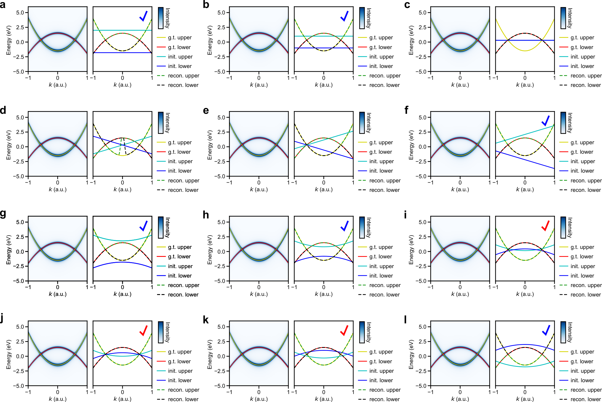
Supplementary Figure 7: Essential information in initialization for reconstruction. Results from a series of numerical experiments for demonstrating the effects of band-crossing information in the initialization. For clarity, the results are compared against the ground truth (g.t.) band dispersion – double-crossing parabolas – by overplotting in dashed lines. The tuning involves initializing the reconstruction with three sets of common curves: a-c, parallel straight lines, d-f, single-crossing straight lines, and g-l, double parabolas. The red check marks () label the reconstructions with correct crossings, while the blue check marks () label those with anti-crossings. All numerical experiments used the same simulated data from a toy model with double-crossing parabolas containing only the second and zeroth-order terms. For reconstruction experiments, the nearest-neighbor Gaussian width hyperparameter () in the MRF model is tuned, while the relative position of the initial conditions is shifted to each configuration. - 2.
Reconstructing crossing bands: We tested the simplest case of crossing bands with two parabolas of opposite directions of opening (Supplementary Fig. 6b), a recurring pattern in band structures. To recover the dispersion without band index scrambling, the knowledge of crossing needs to be included numerically in the initialization. This means, operationally, that the initialization requires crossing bands at nearby energy values, or that the reconstruction needs a warm-start optimization. For the double-crossing parabolas, the initializations that yield feasible outcomes are generated by slight tuning of the parabola parameters in the range that retains the crossing.
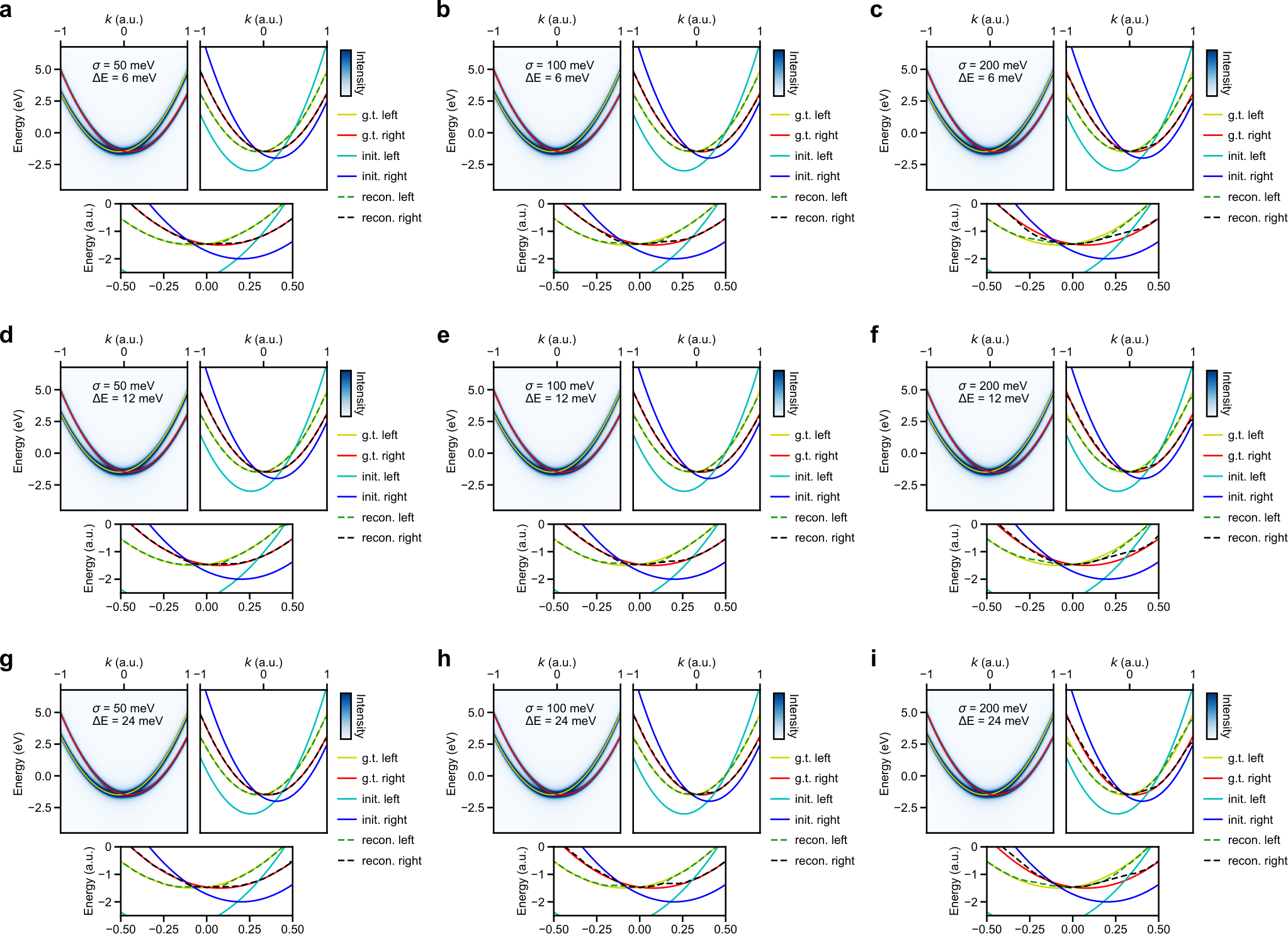
Supplementary Figure 8: The effects of data resolution on reconstruction. Results from a series of numerical experiments for demonstrating the effects of data resolution in either instrument resolution () or energy spacing of data () on the reconstruction accuracy. The results are compared against the ground truth (g.t.) band dispersion – displaced parabolas – by overplotting in dashes lines. The parameter is tuned to 50 meV, 100 meV and 200 meV, while the parameter to 6 meV, 12 meV and 24 meV. In a-i, the synthetic data with ground truth dispersion is shown on the left, the reconstruction outcome is displayed on the right, along with a zoomed-in view near the crossing placed at the bottom. Quantitative values of the reconstruction error are given in Supplementary Table 1. A careful examination over possible scenarios largely confirms this intuition: (1) Initialization with parallel straight lines (without any crossing) only results in non-crossing bands in the reconstruction (Supplementary Fig. 7a-c). When the initial straight line contains the crossings in the ground truth, a symmetry breaking in the reconstruction takes place (Supplementary Fig. 7c), depending on the data and the Gaussian width hyperparameter (). (2) Initialization with two straight lines containing a single crossing yields a reconstruction with at most a single crossing (Supplementary Fig. 7d-f). (3) Initialization with double parabolas yields a reconstruction with at most the same number of crossings within the range of the data (Supplementary Fig. 7g-l). When the reconstruction is successful, the crossings in the initialization are close to the intersection between the two parabolas. Besides, double-crossing parabolas with other parameters from those in Supplementary Fig. 7 are tested and similar outcomes are obtained.
= 50 meV = 100 meV = 200 meV = 6 meV 2.1 3.7 7.5 = 12 meV 2.3 3.8 7.9 = 24 meV 2.4 4.6 10.4 Supplementary Table 1: Reconstruction error in resolution tuning experiments. For each band, the reconstruction error is the root-mean-square error per momentum spacing (unit in meV) between reconstruction and the ground truth, according to Eq. (9). In each numerical experiment, the tabulated reconstruction error is averaged over the corresponding two parabolic bands shown in Supplementary Fig. 8. The columns are the instrument resolution () and the rows are the energy spacing () used to generate the intensity data. The crossing-band model is also an effective test case for resolution effects of the reconstruction algorithm. In this case, a momentum shift is introduced to two parabolic bands to produce the crossing, similar to the Rashba-split surface states of Au [309], which if often used to calibrate experimental resolution in photoemission studies. We conduct a series of numerical experiments using different widths of the instrument resolution and energy spacing to simulate the resolution effect in the synthetic data, using reasonable parameter values. All numerical experiments use a nearest-neighbor Gaussian width hyperparameter within for the reconstruction and no rigid energy shift is introduced. We tabulate the outcomes visually in Supplementary Fig. 8 as gridded figures and quantitatively in Supplementary Table 1 using the reconstruction error (root-mean-square error between ground truth and reconstruction) with the unit in meV. These results show that the reconstruction accuracy, as quantified by the error, has the same trend as the data resolution, which is determined by both the instrument resolution and energy sampling. The instrument resolution appears to have a larger effect on the reconstruction than the energy spacing. In other words, the worse the data resolution ( = 200 meV and = 24 meV being the worst case), the higher the reconstruction error. From visual inspection of the reconstruction in Supplementary Fig. 8, including the zoomed-in region where the crossing is present, it appears that these changes in reconstruction accuracy create essentially no difference in the band dispersion away from the band crossing and only a marginal difference in the vicinity of the band crossing.

Supplementary Figure 9: Validation on 3D synthetic multiband photoemission data. a, Synthetic photoemission data with b, the underlying band structure obtained from LDA-level DFT calculation of WSe2 (only the first 8 valence bands are used here). c, Comparison of two sets of differently scaled (by 0.8 and 1.2 times, respectively) initial conditions with respect to the ground-truth band structure calculation (LDA calc.), shown for a - (left) and a - (right) slice. d,e, Comparison of the average error for energy bands used as initializations (solid dots) and reconstructions (hollow dots). The initializations are constructed by scaling the ground-truth band energies (d) or by using other DFT calculations (e). The reconstructions all have reduced compared with the initialization and is consistent across all energy bands. f,g, Reconstruction, ground truth (LDA), and initialization overlaid on the synthetic data along high-symmetry lines of the hexagonal Brillouin zone, corresponding to two of the cases in d and e, respectively. The energy zeros of the initialization in d-e are aligned with the ground truth via a global shift. h, Comparisons of ground truth (LDA), reconstructed bands, and the differences between initialization (PBE), reconstruction and ground truth (g.t.) for each band. - 3.
Sensitivity of reconstruction to scaled energies as initialization: We scaled the energies of the LDA-DFT band structure of WSe2 (using the first 8 valence bands) around the mean energy of each band (see Supplementary Fig. 9c) for use as the initialization. The accuracy of the reconstruction outcome is evaluated by its average error (Eq. (8) in the main text Methods), calculated with respect to the ground-truth band energies. The results displayed in Supplementary Fig. 9d,f show that the average error and its spread in the reconstruction are reduced from the corresponding values in the initialization. Quantitatively, in the reconstruction, is within the range 20-65 meV, while in the initialization, varies within 45-100 meV for all 8 valence bands.
- 4.
Sensitivity of reconstruction to differently calculated band structures as initialization: We used DFT band structure calculations of WSe2 with PBE, PBEsol and HSE06 exchange-correlation functionals (see Supplementary Section 4) to initialize the reconstruction. The accuracy of the reconstruction is quantified similarly as in the previous numerical experiment using . The results displayed in Supplementary Fig. 9e,g,h show that, despite the huge spread in the average error for the different levels of DFT calculations (used as initialization without global shift alignment of energy zero), the corresponding reconstructions all have average errors at around or below 40 meV for every band. The value of varies by up to 30 meV (i.e. between band #1 and #6) in each set of reconstructed bands, much lower than those in the initialization. The former can be improved by casting the experimental data into finer bins in the preprocessing stage (single-electron events can be binned into various sizes) or interpolating between existing bins, while the latter can be improved by using a continuous probabilistic model [296] to formulate the reconstruction problem, albeit at the cost of much increased computational demand.
The results of the above numerical experiments demonstrate that the reconstruction by MAP optimization converges to a consistent range in the tested scenarios and initializations. It should be noted here that the fundamental accuracy in reconstruction reported here is still limited by the coordinate spacings of the data along all dimensions and the discrete nature of the MRF model (the output is centered only at the bin locations).
2.5 Computational benchmarks
We used the available synthetic photoemission datasets based on the computed band structure of WSe2 to construct benchmarks. The synthesis made use of the approach described in Supplementary Section 2.1. The two datasets used here, taken from [310], exhibit different characteristics, which may be qualitatively described using the energy range of an energy band. The more overlap in the energy range between two energy bands, the more likely they have crossings (or anti-crossings). The dataset-specific information is as follows:
- •
The synthetic dataset of the WSe2 K-point shows close proximity in energies between neighboring momentum locations. The energy ranges of all energy bands have no or up to a moderate degree of overlap. The dataset size is 30 30 500 and contains 900 photoemission spectra.
- •
The synthetic high-symmetry line dataset of WSe2 exhibits large dispersion. Since the high-symmetry line often represents the direction with the most dispersion in the band structure, the energy ranges of all energy bands are strongly overlapping. The dataset size is 186 500 and contains 186 photoemission spectra.
In both cases, the ground-truth band dispersions are taken from the LDA-DFT calculation, including all 14 valence bands, while the initializations for benchmarking both band reconstruction approaches are the PBE-DFT calculation (partial example see Supplementary Fig. 9g). Using these two datasets, we compare the reconstruction algorithms based on pointwise fitting (using the code in [259]) and MRF as introduced in this work. The hyperparameters for the pointwise fitting involve only the band-wise relative shifts applied in each band initialization (14 hyperparameters in total for 14 bands), which were tuned for each band sequentially from band #1 to band #14 using an expanding window approach (introduced in [259]). For the MRF reconstruction, the hyperparameters (including the band-wise shift and the width of the nearest-neighbor Gaussian prior, 28 hyperparameters in total for 14 bands) were tuned individually while reconstructing each band. The hyperparameter tuning made use of grid search through a range of preset values, using the root-mean-squared (RMS) error for determining the final choice. All benchmarks were run on an on-premises computing server (Dell PowerEdge R840), equipped with four Intel Xeon Gold 6150 multicore CPUs.
Dataset 1 Pointwise line fitting 2 MRF reconstruction (s) (s) (eV) (eV) (s) (s) (eV) (eV) WSe2 K point 900 1-2 42 421 4.6e-4 3.2e-4 6.6e-1 34 5.8e-3 4.1e-3 3-4 168 2519 3.6e-1 1.4e-1 1.0 96 1.1e-2 5.5e-3 5-8 412 11964 1.5e-1 5.3e-2 2.2 134 6.0e-2 2.1e-2 9-14 2792 78181 3.6e-1 9.6e-2 3.8 236 7.8e-2 2.1e-2 WSe2 high- symmetry line 186 1-2 13 191 3.6e-1 2.1e-1 3.9e-1 32 1.1e-2 2.0e-2 3-4 46 692 6.2e-1 2.9e-1 2.9e-1 31 1.9e-2 1.8e-2 5-8 385 8858 5.5e-1 1.7e-1 8.6e-1 56 3.0e-2 1.4e-2 9-14 872 27889 3.3 8.7e-1 1.6 109 4.1e-2 1.1e-2 Supplementary Table 2: Algorithm comparison using benchmark datasets. Two synthetic datasets with different number of spectra () and the range of band indices () are used for benchmarking the algorithm performance. The per-band, per-spectrum reconstruction error () is calculated using Eq. (23). The instability () quantifies the variation of the fitting residuals among all spectra within a dataset using the standard deviation of residuals, as in Eq. (24). The single-run time () is the averaged elapsed time in a single execution of fitting, while the tuning time () is the total time used for tuning the parameters to reach the final outcome. Both methods use DFT calculation as the initialization for the band positions. The computational performance of the two algorithms was evaluated using four different metrics as summarized in Supplementary Table 2. The timing metrics provided in the table include the average single-run computing time in each dataset as well as the total computing time of the hyperparameter tuning, which covers all grid search steps of the energy bands (indices described in ) in every benchmarking stage. The computing time for the single runs of each dataset shows a clear advantage of the machine learning-based algorithm and the gap between the two algorithms only widens as the number of bands increases. The accuracy of the reconstruction is quantified by an RMS error averaged over all reconstructed bands and spectra, following the expression for “band delta” in [292].
(23) where is the number of bands and the subscript is the band index. The instability is quantified by the standard deviation of the residual (difference between the ground truth and reconstructed energy dispersion), .
(24) where the overline indicates the mean. This metric has been used in earth sciences to quantify surface roughness [261, 311], which may be interpreted similarly in our case. The difference is that the roughness in the reconstructed surface is largely due to the instability of the optimization, besides the quality of the data, because band dispersions are generally smooth and continuous. In the main text Fig. 4, these tabulated metrics are normalized by the number of spectra to allow comparison between datasets, as is also adopted in [259]. We interpret the results in Supplementary Table 2 in the following two aspects:
- •
Computing time ( and ): For the same dataset, the single-run computing time of the MRF reconstruction is about 2-3 orders of magnitude faster than distributed pointwise fitting. Even with the hyperparameter tuning included, the MRF reconstruction still runs 1-2 orders of magnitude faster, although the MRF reconstruction requires tuning one more hyperparameter than the pointwise fitting approach for each band.
- •
Reconstruction quality ( and ): The substantially higher reconstruction error and instability for pointwise fitting are due to the lack of connectivity between neighbors come primarily from the (theoretical) initialization. Because for each band, even though a global energy shift hyperparameter is tuned, it cannot guarantee that everywhere locally the shift is optimal for band reconstruction, resulting in scrambled band indices in the local patches that the fitting fails. This scenario is a failure mode of the pointwise fitting-based reconstruction as illustrated in [259] for real-world experimental data. This limitation of the pointwise fitting approach is less pronounced when the energy range overlap between bands is small, yet becomes more severe in the high-symmetry line dataset, where the strong energy range overlap and the multiple band crossing (or anti-crossing) make the reconstruction harder to resolve by tuning a single energy shift parameter. The probabilistic framework of the MRF approach largely circumvents this limitation using a physical prior that accounts for the proximity of the neighboring energy values and achieves high stability in the reconstruction.
- •
3 Reconstruction for other datasets
To test the functionality of our MRF reconstruction algorithm on other materials, we have acquired photoemission band mapping datasets from gold (Au), a metal, and bismuth tellurium selenide (Bi2Te2Se), a topological insulator. Due to the complexity of the electronic structure of these materials, we focus here on reconstructing a subset of the energy bands of these two materials that are pronounced within the measured energy range. Besides, we simulated the case where the electron self-energy strongly modifies the band dispersion that results in kink anomalies [312, 313, 226].
3.1 Near-gap electronic bands of a topological insulator (Bi2Te2Se)
The dataset for Bi2Te2Se was measured at room temperature at the Fritz Haber Institute in Berlin using a momentum microscope (SPECS METIS 1000). The sample growth method was previously described in [314]. A clean surface was prepared in vacuum by in situ cleaving with Scotch tape. During the measurement, light excitation of 800 nm was used to examine ultrafast dynamics. The temporal features were ignored here and averaged to improve the signal-to-noise ratio of the data. The photoemission spectra of Bi2Te2Se near the Fermi level feature a topologically-protected surface state (SS) that intersects at the Dirac point (DP) [263] as shown in main text Fig. 6a-b. The SS bridges the valence and conduction bands, an identifiable and prominent feature for this class of materials directly measurable via photoemission [263, 315].
Preprocessing of the 3D band mapping data follows the procedure for WSe2 data described in the main text, except that the rotational symmetrization is only threefold, due to the symmetry of the material. We used numerical initializations from simple functions such as paraboloid and Gaussian in 2D, instead of any first-principles calculation. The reconstructed energy dispersions were smoothed using Chambolle’s total variation denoising algorithm [316] implemented in scikit-image [317], removing the high-frequency noise as a result of the Poisson statistics of the photoemission data. As shown in main text Fig. 6c, the simple initializations we chose are sufficient to reconstruct the complex dispersion from the first two valence bands, the SS and parts of the first conduction band occupied by the excited electronic population. The appearance of the first conduction band for Bi2Te2Se is a result of photoexcitation [318]. The reconstructed bands show sixfold symmetry and warping in agreement with previous theoretical investigations [263, 315], which is more straightforwardly visualized in 2D and 3D as in main text Fig. 6d-e. For the dispersion surfaces of the SS and the conduction band, we truncated the dispersion to a realistic energy range not far from the photon energies of the excitation light pulses.
3.2 Bulk electronic bands of gold (Au)
The Au dataset was measured at 100 K at the SGM-3 beamline [319] of the 3rd-generation synchrotron radiation facility ASTRID2 in Aarhus, Denmark. The Au samples were purchased from MaTecK GmbH with a (111) surface. The sample preparation procedure has been previously described [320]. The photoemission data were measured along the high-symmetry direction (KM) of Au(111), which exhibits a hexagonal symmetry in the surface Brillouin zone [321] (indicated with an overbar over each symmetry label) similar to WSe2. As shown in main text Fig. 6f, the collection of energy bands present in the photoemission data for Au(111) includes the surface states (SSs), which, at sufficient momentum and energy resolution, are composed of momentum-shifted parabolas [309]. The photon energy for the photoemission measurement is 80 eV, which resolves the bands and the surface states poorly but the bulk bands better. The bands and the bands are the low-energy bulk electronic bands of Au.
Before reconstruction, the Au data has been preprocessed using contrast enhancement and intensity smoothing as described in the main text for the WSe2 data before reconstruction. The reconstruction used existing DFT calculations, which feature a Au(111) slab containing five Au layers constructed according to [322], as initialization to retrieve parts of the bands that are resolvable within the current dataset. The comparison between initialization and reconstruction is shown in main text Fig. 6g. The choice of the initialization is a consistent set of energy bands (i.e. produced by the same slab) from DFT calculations of Au(111) slabs in the energy range close to the noticeable bands in the photoemission data. Although traditionally, slab calculations along with overplotting are used to approximate the total band width, we have shown that our reconstruction approach can detect existing band-like dispersive features in these highly congested data.

3.3 Reconstructing the kink anomaly
Kink anomalies are a kind of feature for electron-phonon interaction in photoemission signals [225, 226] found in various materials [312, 323, 313]. To test the reconstruction performance, we simulated the photoemission signal for a kink anomaly using the full spectral function introduced in Eq. (11). The real part of the electron self-energy is calculated using the Eliashberg function [324] represented as an Einstein mode (i.e. single-phonon mode with a delta-function-like frequency response) [325], which appears near the Fermi level. Further details of the computational model can be found in the Jupyter notebooks within the associated compute capsule. The presence of an Einstein mode in the spectral function results in a phonon-induced kink at around - 0.1 eV.
The outcome of the reconstruction, shown in Supplementary Fig. 10, indicates that the MRF model can recover faithfully the quasiparticle dispersion including the shape of the kink anomaly. The reconstruction can simply be initialized with a flat line, which produces identical results from initialization with a linear dispersion that could represent prior knowledge of the algorithm user. The results show that for strongly dispersive energy bands with almost vertical dispersion along the energy direction, reconstruction along the energy direction (i.e. treating the data as a collection of momentum distribution functions) yields a better outcome. This is because the existence of the kink violates the one-to-one mapping between the band energy, , and the photoelectron momentum, (see Supplementary Fig. 10a-b). In these cases, the reconstruction is still viable using the momentum distribution function as the likelihood in the MRF model, which effectively amounts to transposing the image and swapping the momentum and energy coordinates, while the same optimization algorithm described in this work for the EDC-based approach can be reused to obtain the correct quasiparticle dispersion (see Supplementary Fig. 10c-d).
4 Band structure calculations
4.1 DFT calculations
The crystal structure of bulk WSe2 with 2 stacking (2-WSe2) belongs to the P63/mmc space group and consists of two Se-W-Se triatomic layers as shown in Supplementary Fig. 11. The stacking order of the two hexagonal layers is --- and the long -axis is oriented perpendicular to the layers. Electronic structure calculations were performed within DFT using the local density approximation (LDA), the generalized-gradient approximation (GGA-PBE and GGA-PBEsol), and hybrid (HSE06) exchange-correlation functionals as implemented in FHI-aims [291]. The atomic orbitals basis sets, the integration grids and the Hartree potential employed for all calculations are according to the default “tight” numerical settings of FHI-aims. A 16164 uniform k-gird was used to sample the Brillouin zone. The Broyden-Fletcher-Goldfarb-Shanno optimization algorithm was used to relax the atomic positions until the residual force component per atom was less than 10-2 eV/Å. Supplementary Table 3 shows the optimized lattice constants, and , as obtained by the evaluation of the analytical stress tensor [326] using different exchange-correlation functionals. In all BS calculations, we included the effect of spin-orbit coupling, which is known to introduce a large splitting of the outermost valence states of bulk 2-WSe2 [327].

| xc-functional | LDA | PBE | PBEsol | HSE06 | Experiment | ||||||||
| (Å) | 3.250 | 3.317 | 3.269 | 3.295 | 3.28 | ||||||||
| (Å) | 12.827 | 14.921 | 13.211 | 13.863 | 12.98 | ||||||||
| Spin-orbit splitting at K (eV) |
|
|
|
|
0.5 3 | ||||||||
| Band gap (eV) |
|
|
|
|
1.219 4 |
The calculated BSs of bulk 2-WSe2 using different levels of approximation for the exchange-correlation (XC) functional are shown in Supplementary Fig. 12. For each XC functional, the calculations were performed on (1) fully optimized structures (black lines), and on (2) optimized structures by fixing the lattice parameters of the unit cell to the experimental values (colored lines). All calculations using different XC functionals reveal an indirect band gap with the conduction band minimum located along the -K path ( and K being the bulk equivalents of the and high-symmetry points). For both sets of optimized structures, the LDA results reveal a valence band maximum at the point, compatible with experimental measurements, while the PBE, PBEsol, and HSE06 band structures obtained for fully optimized structures exhibit a valence band maximum at the K point. Nevertheless, fixing the unit cell dimensions at the experimental lattice constants reproduces the experimental behavior that the valence band maximum resides at the point. The difference between the two sets of calculations obtained using PBE, PBEsol, and HSE06 functionals is attributed to the overestimation of the lattice parameter and the residual strain along the -axis [329]. The calculated indirect band gaps and the spin-orbit splitting of the two topmost valence states at the K point using both sets of optimized structures are shown in Supplementary Table 3.

4.2 Brillouin zone tiling
The generation of a large and densely sampled patch of energy bands covering the first Brillouin zone and beyond is crucial for initializing the MRF model. To balance the computational cost using different XC functionals with the dense sampling similar to the experimental data grid, we used the symmetry properties of the Brillouin zone to tile the calculated momentum-space rectangular patch that covers the , K and M points of the Brillouin zone. The hexagonal Brillouin zone of WSe2 has a sixfold rotation symmetry axis and two independent mirror planes in the (, ) coordinates. The initial rectangular patch is first symmetrized about the two mirror planes in the -K and -M directions to form a larger patch, which is then rotated by and , respectively, and combined with the original mirror-symmetrized patch. The composite patch is then shifted along all six -M directions by one unit cell distance and the result is cut to the required shape compatible with photoemission data.
5 Band structure informatics
5.1 Global structure descriptors
We use informatics tools for data retrieval, representation and comparison for entire bands. We extend the examples given in main text Fig. 3b to other bands of WSe2 reconstructed in the present work. Supplementary Fig. 13 displays the band-wise comparison of dispersion surfaces within other DFT calculations. These results contain similar features as in main text Fig. 3a and c, reaffirming that the geometric featurization provides a sparse representation of the band dispersions and that the dispersion similarities are largely preserved despite the use of different exchange-correlation functionals in the DFT calculations. They may, therefore, be regarded as general features of the WSe2 band structure.
In Supplementary Fig. 14, we demonstrate numerically the approximation capability of the hexagonal ZP basis set to all 14 valence bands of WSe2. Despite the stark differences in energy dispersion, the approximation to reconstructed bands (Supplementary Fig. 14a-d) and theoretical band structure at the level of LDA-DFT (Supplementary Fig. 14e-h) show comparable convergence rates. Quantitatively, the approximation using hexagonal ZPs ordered by the magnitude of the corresponding coefficients (i.e. coefficient order) converges to within 10-30 meV/band within 50 polynomial basis terms, substantially faster than using the default order (see also Fig. 3b for reference). The remaining errors are on par with the finite step size along the energy axis in the data ( 18 meV) that results in the imperfect smoothness of the reconstructed bands. This further proves that the hexagonal ZPs can provide an accurate and sparse approximation for the band structure data. The trend of convergence between these two types of polynomial ordering is further illustrated in Supplementary Fig. 14i-j in the momentum path along high-symmetry lines of the reconstructed band structure.
5.2 Local structure descriptors
Local structural information includes energy gaps, effective masses, warpings, (avoided) crossings, etc. We extracted some of their associated parameters at and around three high-symmetry points (, , and , see main text Fig. 5a) and compiled the results in Supplementary Table 4. The dispersions and band structure parameters from the MAP reconstruction are compared with those extracted by the line-by-line fitting of the EDCs, which used the band energies from the reconstruction as initialization to improve robustness. Around , two spectral peaks corresponding to two spin-split bands were fit simultaneously, while around and , four were fit simultaneously due to the spectral proximity of the first four valence bands (see Supplementary Fig. 5). The fitting is carried out using a linear superposition of Voigt lineshapes and the lmfit package [330] with the reconstructed band energy as initialization (but not fixed). The fitting procedure iterates over the EDCs (e.g. a total of 5050 EDCs for the patch around ). Unstable fits yielding erratic results (e.g. if differing greatly from neighboring values) are re-fit with either algorithmically or manually adjusted initialization. Supplementary Table 4 shows that the local structural information from reconstruction is generally consistent with those obtained by iterative pointwise fitting while differing from DFT calculations. The deviations in the size of energy gaps at and between reconstruction and pointwise fitting lie in the same range as the momentum-averaged reconstruction errors (see Supplementary Section 2), which are due to the finite coordinate spacing in the data ( 18 meV in energy).
| Symmetry point | Parameter | LDA recon. 1 | Line fitting 2 | LDA 3 | HSE06 3 |
| 0.62 | 0.60 | 0.49 | 0.42 | ||
| 0.74 | 0.78 | 0.64 | 0.54 | ||
| (eV) | 5.3 | 5.8 | 6.2 | 4.5 | |
| (eV) | 4.0 | 3.9 | 3.9 | 3.2 | |
| (meV) | 419 | 446 | 485 | 467 | |
| 0.71 | 0.72 | 0.25 | 0.17 | ||
| 1.6 | 1.5 | 1.1 | 0.90 | ||
| (meV) | 352 | 338 | 127 | 48 | |
| 0.82 | 1.1 | 0.81 | 1.0 |
- 1
Using band dispersion reconstructed globally by the proposed probabilistic machine learning algorithm with DFT calculation at the LDA level as the initialization.
- 2
Using band dispersion from iterative lineshape fitting of the energy distribution curves (in a region around the corresponding high-symmetry points).
- 3
With fully optimized structure, see Supplementary Table 3.
The region extracted around (see main text Fig. 5d-e) contains about 10% of the distance of . Due to the strong trigonal warping (TW) effect in this class of materials, the effective masses and the TW parameters around were fit simultaneously in 2D using the momentum-space model derived from kp theory [249].
| (25) |
Here, q is the momentum vector k recentered on a particular (or ) point by translation, is the effective mass of the hole at point, is the magnitude of the TW (named in [249]), is the polar angle in the coordinate system centered on a (or ) point, is an auxiliary fitting parameter used to accommodate the orientation of the TW with respect to the pixel coordinates defined by the rectangular region of interest, accounts for the energy offset. The energy gaps at () and () are illustrated in main text Fig. 5 (b and d), respectively. The (or ) point situates at a saddle point of the dispersion surface (first valence band), as shown in main text Fig. 5b-c. Its lower symmetry (compared with , and ) means that the effective masses exhibits anisotropy, with opposite signs and magnitude along the and directions. We fit the dispersion locally using a model that also accounts for the spin-orbit interaction involving a linear momentum-dependent shift (Eq. 14 in [249]). The second valence band is not fitted at due to the pronounced dispersion modulation by interband coupling unaccounted for in the existing saddle-shaped model. At around , a single effective mass is extracted by fitting a paraboloid to a local patch of the dispersion surface.
References
- [221] Eric. Isaacs and Chris Wolverton “Inverse Band Structure Design via Materials Database Screening: Application to Square Planar Thermoelectrics” In Chemistry of Materials 30.5, 2018, pp. 1540–1546 DOI: 10.1021/acs.chemmater.7b04496
- [222] E.. Marin et al. “Modeling of Electron Devices Based on 2-D Materials” In IEEE Transactions on Electron Devices 65.10, 2018, pp. 4167–4179 DOI: 10.1109/TED.2018.2854902
- [223] L.. Bouckaert, R. Smoluchowski and E. Wigner “Theory of Brillouin Zones and Symmetry Properties of Wave Functions in Crystals” In Physical Review 50.1, 1936, pp. 58–67 DOI: 10.1103/PhysRev.50.58
- [224] T.-C. Chiang and F. Seitz “Photoemission spectroscopy in solids” In Annalen der Physik 10.1-2, 2001, pp. 61–74 DOI: 10.1002/1521-3889(200102)10:1/2¡61::AID-ANDP61¿3.0.CO;2-G
- [225] Andrea Damascelli, Zahid Hussain and Zhi-Xun Shen “Angle-resolved photoemission studies of the cuprate superconductors” In Reviews of Modern Physics 75.2, 2003, pp. 473–541 DOI: 10.1103/RevModPhys.75.473
- [226] Hongyun Zhang et al. “Angle-resolved photoemission spectroscopy” In Nature Reviews Methods Primers 2.1, 2022, pp. 54 DOI: 10.1038/s43586-022-00133-7
- [227] Gerd Schönhense, Katerina Medjanik and Hans-Joachim Elmers “Space-, time- and spin-resolved photoemission” In Journal of Electron Spectroscopy and Related Phenomena 200, 2015, pp. 94–118 DOI: 10.1016/j.elspec.2015.05.016
- [228] K. Medjanik et al. “Direct 3D mapping of the Fermi surface and Fermi velocity” In Nature Materials 16.6, 2017, pp. 615–621 DOI: 10.1038/nmat4875
- [229] M. Puppin et al. “Time- and angle-resolved photoemission spectroscopy of solids in the extreme ultraviolet at 500 kHz repetition rate” In Review of Scientific Instruments 90.2, 2019, pp. 023104 DOI: 10.1063/1.5081938
- [230] Alexandre Gauthier et al. “Tuning time and energy resolution in time-resolved photoemission spectroscopy with nonlinear crystals” In Journal of Applied Physics 128.9, 2020, pp. 093101 DOI: 10.1063/5.0018834
- [231] J.. Riley et al. “Direct observation of spin-polarized bulk bands in an inversion-symmetric semiconductor” In Nature Physics 10.11, 2014, pp. 835–839 DOI: 10.1038/nphys3105
- [232] M.. Bahramy et al. “Ubiquitous formation of bulk Dirac cones and topological surface states from a single orbital manifold in transition-metal dichalcogenides” In Nature Materials 17.1, 2018, pp. 21–28 DOI: 10.1038/nmat5031
- [233] Niels.. Schröter et al. “Chiral topological semimetal with multifold band crossings and long Fermi arcs” In Nature Physics 15.8, 2019, pp. 759–765 DOI: 10.1038/s41567-019-0511-y
- [234] T. Valla et al. “Evidence for Quantum Critical Behavior in the Optimally Doped Cuprate Bi2Sr2CaCu2O8+δ” In Science 285.5436, 1999, pp. 2110–2113 DOI: 10.1126/science.285.5436.2110
- [235] G. Levy et al. “Deconstruction of resolution effects in angle-resolved photoemission” In Physical Review B 90.4, 2014, pp. 045150 DOI: 10.1103/PhysRevB.90.045150
- [236] P. Zhang et al. “A precise method for visualizing dispersive features in image plots” In Review of Scientific Instruments 82.4, 2011, pp. 043712 DOI: 10.1063/1.3585113
- [237] Yu He, Yan Wang and Zhi-Xun Shen “Visualizing dispersive features in 2D image via minimum gradient method” In Review of Scientific Instruments 88.7, 2017, pp. 073903 DOI: 10.1063/1.4993919
- [238] Han Peng et al. “Super resolution convolutional neural network for feature extraction in spectroscopic data” In Review of Scientific Instruments 91.3, 2020, pp. 033905 DOI: 10.1063/1.5132586
- [239] Younsik Kim et al. “Deep learning-based statistical noise reduction for multidimensional spectral data” In Review of Scientific Instruments 92.7, 2021, pp. 073901 DOI: 10.1063/5.0054920
- [240] Simon Moser “An experimentalist’s guide to the matrix element in angle resolved photoemission” In Journal of Electron Spectroscopy and Related Phenomena 214, 2017, pp. 29–52 DOI: 10.1016/j.elspec.2016.11.007
- [241] Kevin. Murphy “Machine Learning: A Probabilistic Perspective” MIT Press, 2012
- [242] Zoubin Ghahramani “Probabilistic machine learning and artificial intelligence” In Nature 521.7553, 2015, pp. 452–459 DOI: 10.1038/nature14541
- [243] Chaohui Wang, Nikos Komodakis and Nikos Paragios “Markov Random Field modeling, inference & learning in computer vision & image understanding: A survey” In Computer Vision and Image Understanding 117.11, 2013, pp. 1610–1627 DOI: https://doi.org/10.1016/j.cviu.2013.07.004
- [244] Mary Comer and Jeff Simmons “The Markov Random Field in Materials Applications: A synoptic view for signal processing and materials readers” In IEEE Signal Processing Magazine 39.1, 2022, pp. 16–24 DOI: 10.1109/MSP.2021.3123564
- [245] Kevin Kaufmann et al. “Crystal symmetry determination in electron diffraction using machine learning” In Science 367.6477, 2020, pp. 564–568 DOI: 10.1126/science.aay3062
- [246] Vincent Stimper et al. “Multidimensional Contrast Limited Adaptive Histogram Equalization” In IEEE Access 7, 2019, pp. 165437–165447 DOI: 10.1109/ACCESS.2019.2952899
- [247] M. Traving et al. “Electronic structure of WSe2: A combined photoemission and inverse photoemission study” In Physical Review B 55.16, 1997, pp. 10392–10399 DOI: 10.1103/PhysRevB.55.10392
- [248] Th. Finteis et al. “Occupied and unoccupied electronic band structure of WSe2” In Physical Review B 55.16, 1997, pp. 10400–10411 DOI: 10.1103/PhysRevB.55.10400
- [249] Andor Kormányos et al. “k · p theory for two-dimensional transition metal dichalcogenide semiconductors” In 2D Materials 2.2, 2015, pp. 022001 DOI: 10.1088/2053-1583/2/2/022001
- [250] John. Perdew and Karla Schmidt “Jacob’s ladder of density functional approximations for the exchange-correlation energy” In AIP Conference Proceedings 577 AIP, 2001, pp. 1–20 DOI: 10.1063/1.1390175
- [251] Dorothea Golze, Marc Dvorak and Patrick Rinke “The GW Compendium: A Practical Guide to Theoretical Photoemission Spectroscopy” In Frontiers in Chemistry 7:377, 2019 DOI: 10.3389/fchem.2019.00377
- [252] Marios Zacharias, Matthias Scheffler and Christian Carbogno “Fully anharmonic nonperturbative theory of vibronically renormalized electronic band structures” In Physical Review B 102.4, 2020, pp. 045126 DOI: 10.1103/PhysRevB.102.045126
- [253] Dengsheng Zhang and Guojun Lu “Review of shape representation and description techniques” In Pattern Recognition 37.1, 2004, pp. 1–19 DOI: 10.1016/j.patcog.2003.07.008
- [254] A. Khotanzad and Y.H. Hong “Invariant image recognition by Zernike moments” In IEEE Transactions on Pattern Analysis and Machine Intelligence 12.5, 1990, pp. 489–497 DOI: 10.1109/34.55109
- [255] Virendra. Mahajan and Guang-ming Dai “Orthonormal polynomials in wavefront analysis: analytical solution” In Journal of the Optical Society of America A 24.9, 2007, pp. 2994 DOI: 10.1364/JOSAA.24.002994
- [256] Lauri Himanen, Amber Geurts, Adam Foster and Patrick Rinke “Data‐Driven Materials Science: Status, Challenges, and Perspectives” In Advanced Science, 2019, pp. 1900808 DOI: 10.1002/advs.201900808
- [257] M.. Horton, S. Dwaraknath and K.. Persson “Promises and perils of computational materials databases” In Nature Computational Science 1.1, 2021, pp. 3–5 DOI: 10.1038/s43588-020-00016-5
- [258] Armen Kiureghian and Ove Ditlevsen “Aleatory or epistemic? Does it matter?” In Structural Safety 31.2, 2009, pp. 105–112 DOI: 10.1016/j.strusafe.2008.06.020
- [259] Rui Xian, Ralph Ernstorfer and Philipp Pelz “Scalable multicomponent spectral analysis for high-throughput data annotation” In arXiv, 2021, pp. 2102.05604 arXiv: http://arxiv.org/abs/2102.05604
- [260] Jorge Nocedal and Stephen. Wright “Numerical Optimization” Springer New York, 2006 DOI: 10.1007/978-0-387-40065-5
- [261] Mark. Smith “Roughness in the Earth Sciences” In Earth-Science Reviews 136, 2014, pp. 202–225 DOI: 10.1016/j.earscirev.2014.05.016
- [262] Huaihong Guo et al. “Double resonance Raman modes in monolayer and few-layer MoTe2” In Physical Review B 91.20, 2015, pp. 205415 DOI: 10.1103/PhysRevB.91.205415
- [263] Joseph. Heremans, Robert. Cava and Nitin Samarth “Tetradymites as thermoelectrics and topological insulators” In Nature Reviews Materials 2.10, 2017, pp. 17049 DOI: 10.1038/natrevmats.2017.49
- [264] “Multi-Band Effective Mass Approximations” 94, Lecture Notes in Computational Science and Engineering Springer, 2014 DOI: 10.1007/978-3-319-01427-2
- [265] Matthias Scheffler et al. “FAIR data enabling new horizons for materials research” In Nature 604.7907, 2022, pp. 635–642 DOI: 10.1038/s41586-022-04501-x
- [266] A.. Kordyuk et al. “Bare electron dispersion from experiment: Self-consistent self-energy analysis of photoemission data” In Physical Review B 71.21, 2005, pp. 214513 DOI: 10.1103/PhysRevB.71.214513
- [267] Marcus. Noack et al. “Gaussian processes for autonomous data acquisition at large-scale synchrotron and neutron facilities” In Nature Reviews Physics 3.10, 2021, pp. 685–697 DOI: 10.1038/s42254-021-00345-y
- [268] Samuel Beaulieu et al. “Ultrafast dynamical Lifshitz transition” In Science Advances 7.17, 2021, pp. eabd9275 DOI: 10.1126/sciadv.abd9275
- [269] Davide Curcio et al. “Accessing the Spectral Function in a Current-Carrying Device” In Physical Review Letters 125.23, 2020, pp. 236403 DOI: 10.1103/PhysRevLett.125.236403
- [270] Neil. Wilson et al. “Determination of band offsets, hybridization, and exciton binding in 2D semiconductor heterostructures” In Science Advances 3.2, 2017, pp. e1601832 DOI: 10.1126/sciadv.1601832
- [271] Søren Ulstrup et al. “Nanoscale mapping of quasiparticle band alignment” In Nature Communications 10.1, 2019, pp. 3283 DOI: 10.1038/s41467-019-11253-2
- [272] R.A. Ewings et al. “Horace : Software for the analysis of data from single crystal spectroscopy experiments at time-of-flight neutron instruments” In Nuclear Instruments and Methods in Physics Research Section A: Accelerators, Spectrometers, Detectors and Associated Equipment 834, 2016, pp. 132–142 DOI: 10.1016/j.nima.2016.07.036
- [273] C.. Whittaker et al. “Exciton Polaritons in a Two-Dimensional Lieb Lattice with Spin-Orbit Coupling” In Physical Review Letters 120.9, 2018, pp. 097401 DOI: 10.1103/PhysRevLett.120.097401
- [274] Andreas Frölich et al. “Frequency-Resolved Reciprocal-Space Mapping of Visible Spontaneous Emission from 3D Photonic Crystals” In Advanced Optical Materials 2.9, 2014, pp. 849–853 DOI: 10.1002/adom.201400150
- [275] Iban Amenabar et al. “Hyperspectral infrared nanoimaging of organic samples based on Fourier transform infrared nanospectroscopy” In Nature Communications 8.1, 2017, pp. 14402 DOI: 10.1038/ncomms14402
- [276] Laura von Rueden et al. “Informed Machine Learning - A Taxonomy and Survey of Integrating Prior Knowledge into Learning Systems” In IEEE Transactions on Knowledge and Data Engineering, 2021, pp. 1–1 DOI: 10.1109/TKDE.2021.3079836
- [277] A. Oelsner et al. “Microspectroscopy and imaging using a delay line detector in time-of-flight photoemission microscopy” In Review of Scientific Instruments 72.10, 2001, pp. 3968–3974 DOI: 10.1063/1.1405781
- [278] R. Xian et al. “An open-source, end-to-end workflow for multidimensional photoemission spectroscopy” In Scientific Data 7.1, 2020, pp. 442 DOI: 10.1038/s41597-020-00769-8
- [279] SPECS GmbH “METIS 1000 Brochure”, https://www.specs-group.com/fileadmin/user_upload/products/brochures/SPECS_Brochure-METIS_RZ_web.pdf, 2019
- [280] Rui Xian, Laurenz Rettig and Ralph Ernstorfer “Symmetry-guided nonrigid registration: The case for distortion correction in multidimensional photoemission spectroscopy” In Ultramicroscopy 202, 2019, pp. 133–139 DOI: 10.1016/j.ultramic.2019.04.004
- [281] J Kittler and J Föglein “Contextual classification of multispectral pixel data” In Image and Vision Computing 2.1, 1984, pp. 13–29 DOI: https://doi.org/10.1016/0262-8856(84)90040-4
- [282] Martín Abadi et al. “TensorFlow: Large-Scale Machine Learning on Heterogeneous Distributed Systems” In arXiv, 2016, pp. 1603.04467v2 arXiv: http://arxiv.org/abs/1603.04467
- [283] Stan Li “Markov Random Field Modeling in Image Analysis”, Advances in Pattern Recognition Springer, 2009
- [284] Vincent Stimper and Rui Xian “fuller”, https://github.com/mpes-kit/fuller URL: https://github.com/mpes-kit/fuller
- [285] Yoyo Hinuma et al. “Band structure diagram paths based on crystallography” In Computational Materials Science 128, 2017, pp. 140–184 DOI: 10.1016/j.commatsci.2016.10.015
- [286] D.. Ceperley and B.. Alder “Ground State of the Electron Gas by a Stochastic Method” In Physical Review Letters 45.7, 1980, pp. 566–569 DOI: 10.1103/PhysRevLett.45.566
- [287] John. Perdew and Yue Wang “Accurate and simple analytic representation of the electron-gas correlation energy” In Physical Review B 45.23, 1992, pp. 13244–13249 DOI: 10.1103/PhysRevB.45.13244
- [288] John. Perdew, Kieron Burke and Matthias Ernzerhof “Generalized Gradient Approximation Made Simple” In Physical Review Letters 77.18, 1996, pp. 3865–3868 DOI: 10.1103/PhysRevLett.77.3865
- [289] John. Perdew et al. “Restoring the Density-Gradient Expansion for Exchange in Solids and Surfaces” In Physical Review Letters 100.13, 2008, pp. 136406 DOI: 10.1103/PhysRevLett.100.136406
- [290] Jochen Heyd, Gustavo. Scuseria and Matthias Ernzerhof “Hybrid functionals based on a screened Coulomb potential” In The Journal of Chemical Physics 118.18, 2003, pp. 8207–8215 DOI: 10.1063/1.1564060
- [291] Volker Blum et al. “Ab initio molecular simulations with numeric atom-centered orbitals” In Computer Physics Communications 180.11, 2009, pp. 2175–2196 DOI: 10.1016/j.cpc.2009.06.022
- [292] William. Huhn and Volker Blum “One-hundred-three compound band-structure benchmark of post-self-consistent spin-orbit coupling treatments in density functional theory” In Physical Review Materials 1.3, 2017, pp. 033803 DOI: 10.1103/PhysRevMaterials.1.033803
- [293] James. Wyant and Katherine Creath “Basic wavefront aberration theory” In Applied Optics and Optical Engineering Xl Academic Press, 1992, pp. 1–53
- [294] David. Watkins “Fundamentals of matrix computations” Wiley, 2010
- [295] Stefan Hüfner “Photoelectron Spectroscopy”, Advanced Texts in Physics Springer Berlin Heidelberg, 2003 DOI: 10.1007/978-3-662-09280-4
- [296] Christopher. Bishop “Pattern Recognition and Machine Learning” Springer, 2006
- [297] J.. Hammersley and P. Clifford “Markov Fields on Finite Graphs and Lattices” Unpublished, 1971 URL: http://www.statslab.cam.ac.uk/~grg/books/hammfest/hamm-cliff.pdf
- [298] Julian Besag “Spatial Interaction and the Statistical Analysis of Lattice Systems” In Journal of the Royal Statistical Society. Series B (Methodological) 36.2 [Royal Statistical Society, Wiley], 1974, pp. 192–236 URL: http://www.jstor.org/stable/2984812
- [299] Stuart Geman and Donald Geman “Stochastic Relaxation, Gibbs Distributions, and the Bayesian Restoration of Images” In IEEE Transactions on Pattern Analysis and Machine Intelligence 6.6, 1984, pp. 721–741 DOI: 10.1109/TPAMI.1984.4767596
- [300] Julian Besag “On the Statistical Analysis of Dirty Pictures” In Journal of the Royal Statistical Society: Series B (Methodological) 48.3, 1986, pp. 259–279 DOI: 10.1111/j.2517-6161.1986.tb01412.x
- [301] Judea Pearl “Probabilistic Reasoning in Intelligent Systems” Morgan Kaufmann, 1988 DOI: 10.1016/C2009-0-27609-4
- [302] J. Besag “On the statistical analysis of nearest-neighbours” In Proceedings of the European Meeting of Statisticians, Budapest, 1972
- [303] M. Locatelli “A note on the Griewank test function” In Journal of Global Optimization 25.2, 2003, pp. 169–174 DOI: 10.1023/A:1021956306041
- [304] Cristina Bena and Gilles Montambaux “Remarks on the tight-binding model of graphene” In New Journal of Physics 11.9, 2009, pp. 095003 DOI: 10.1088/1367-2630/11/9/095003
- [305] Virendra. Mahajan and Guang-ming Dai “Orthonormal polynomials for hexagonal pupils” In Optics Letters 31.16, 2006, pp. 2462 DOI: 10.1364/OL.31.002462
- [306] H.. van Hulst and J… Reesinck “Line Breadths and Voigt Profiles.” In The Astrophysical Journal 106, 1947, pp. 121 DOI: 10.1086/144944
- [307] Mofreh. Zaghloul and Ahmed. Ali “Algorithm 916: Computing the Faddeyeva and Voigt Functions” In ACM Transactions on Mathematical Software 38.2, 2011, pp. 1–22 DOI: 10.1145/2049673.2049679
- [308] Shuo Dong et al. “Direct measurement of key exciton properties: Energy, dynamics, and spatial distribution of the wave function” In Natural Sciences 1.1, 2021, pp. 1:e10010 DOI: 10.1002/ntls.10010
- [309] S. LaShell, B.. McDougall and E. Jensen “Spin Splitting of an Au(111) Surface State Band Observed with Angle Resolved Photoelectron Spectroscopy” In Physical Review Letters 77.16, 1996, pp. 3419–3422 DOI: 10.1103/PhysRevLett.77.3419
- [310] Rui Xian “pesarxiv”, https://github.com/mpes-kit/pesarxiv URL: https://github.com/mpes-kit/pesarxiv
- [311] Carlos Grohmann, Mike. Smith and Claudio Riccomini “Multiscale Analysis of Topographic Surface Roughness in the Midland Valley, Scotland” In IEEE Transactions on Geoscience and Remote Sensing 49.4, 2011, pp. 1200–1213 DOI: 10.1109/TGRS.2010.2053546
- [312] Feliciano Giustino, Marvin. Cohen and Steven. Louie “Small phonon contribution to the photoemission kink in the copper oxide superconductors” In Nature 452.7190, 2008, pp. 975–978 DOI: 10.1038/nature06874
- [313] Carla Verdi, Fabio Caruso and Feliciano Giustino “Origin of the crossover from polarons to Fermi liquids in transition metal oxides” In Nature Communications 8.1, 2017, pp. 15769 DOI: 10.1038/ncomms15769
- [314] Jian-Li Mi et al. “Phase Separation and Bulk p-n Transition in Single Crystals of Bi2Te2Se Topological Insulator” In Advanced Materials 25.6, 2013, pp. 889–893 DOI: 10.1002/adma.201203542
- [315] Matteo Michiardi et al. “Strongly anisotropic spin-orbit splitting in a two-dimensional electron gas” In Physical Review B 91.3, 2015, pp. 035445 DOI: 10.1103/PhysRevB.91.035445
- [316] Antonin Chambolle “An Algorithm for Total Variation Minimization and Applications” In Journal of Mathematical Imaging and Vision 20.1-2 Springer, 2004, pp. 89–97 DOI: 10.1023/B:JMIV.0000011325.36760.1E
- [317] Stéfan van Walt et al. “scikit-image: image processing in Python” In PeerJ 2, 2014, pp. e453 DOI: 10.7717/peerj.453
- [318] E. Papalazarou et al. “Unraveling the Dirac fermion dynamics of the bulk-insulating topological system Bi2Te2Se” In Physical Review Materials 2.10, 2018, pp. 104202 DOI: 10.1103/PhysRevMaterials.2.104202
- [319] S.V. Hoffmann et al. “An undulator-based spherical grating monochromator beamline for angle-resolved photoemission spectroscopy” In Nuclear Instruments and Methods in Physics Research Section A: Accelerators, Spectrometers, Detectors and Associated Equipment 523.3, 2004, pp. 441–453 DOI: 10.1016/j.nima.2004.01.039
- [320] Maciej Dendzik et al. “Reconstruction-induced trefoil knot Fermi contour of Au(111)” In Physical Review B 94.20, 2016, pp. 201401 DOI: 10.1103/PhysRevB.94.201401
- [321] Christian Tusche, Alexander Krasyuk and Jürgen Kirschner “Spin resolved bandstructure imaging with a high resolution momentum microscope” In Ultramicroscopy 159, 2015, pp. 520–529 DOI: 10.1016/j.ultramic.2015.03.020
- [322] In-Bai Lin, Tony-Hann Sheu and Jia-Han Li “Effects of exchange correlation functional on optical permittivity of gold and electromagnetic responses” In Optics Express 22.25, 2014, pp. 30725 DOI: 10.1364/OE.22.030725
- [323] L. Ortenzi, E. Cappelluti, L. Benfatto and L. Pietronero “Fermi-Surface Shrinking and Interband Coupling in Iron-Based Pnictides” In Physical Review Letters 103.4, 2009, pp. 046404 DOI: 10.1103/PhysRevLett.103.046404
- [324] Junren Shi et al. “Direct Extraction of the Eliashberg Function for Electron-Phonon Coupling: A Case Study of Be(100)” In Physical Review Letters 92.18, 2004, pp. 186401 DOI: 10.1103/PhysRevLett.92.186401
- [325] P.. Allen and R.. Dynes “Transition temperature of strong-coupled superconductors reanalyzed” In Physical Review B 12.3, 1975, pp. 905–922 DOI: 10.1103/PhysRevB.12.905
- [326] Franz Knuth et al. “All-electron formalism for total energy strain derivatives and stress tensor components for numeric atom-centered orbitals” In Computer Physics Communications 190, 2015, pp. 33–50 DOI: https://doi.org/10.1016/j.cpc.2015.01.003
- [327] D. Voß, P. Krüger, A. Mazur and J. Pollmann “Atomic and electronic structure of WSe2 from ab initio theory: Bulk crystal and thin film systems” In Phys. Rev. B 60 American Physical Society, 1999, pp. 14311–14317 DOI: 10.1103/PhysRevB.60.14311
- [328] K Kam, C Chang and D Lynch “Fundamental absorption edges and indirect band gaps in WMoSe2 (01)” In Journal of Physics C: Solid State Physics 17.22 IOP Publishing, 1984, pp. 4031–4040 DOI: 10.1088/0022-3719/17/22/021
- [329] Sujay. Desai et al. “Strain-Induced Indirect to Direct Bandgap Transition in Multilayer WSe2” In Nano Letters 14.8, 2014, pp. 4592–4597 DOI: 10.1021/nl501638a
- [330] Matt Newville et al. “lmfit/lmfit-py 1.0.0” In Zenodo, https://doi.org/10.5281/zenodo.3588521, 2019 DOI: 10.5281/ZENODO.3588521