Magnetic-field modeling with surface currents:
Physical and computational principles of bfieldtools

By taking a line integral of $\psi$ from $\vec{r}_{0}$ to $\vec{r}$ on the surface, we find that the difference in the stream function between the two ends of the path equals the flux of surface current $\vec{j}(\vec{r})$ passing the curve Peeren 2003a

where $d\vec{l}^{\prime}\times\hat{n}^{\prime}$ is a path differential perpendicular to the direction of the path. In consequence, a line integral from a reference point $\vec{r}_{0}$ determines the stream function uniquely on the surface.

From another point of view, the stream function can be interpreted as a surface density of magnetic dipoles normal to the surfacePeeren 2003b; Lopez et al. 2009 (see also Appendix A):

This interpretation of the stream function enables analogies to dipole layers involved in, e.g., volume conductor problems and the calculation of magnetic scalar potentials for divergence-free surface currents.

As the surface current density is assumed divergence-free everywhere, the flux of current through any boundary on the surface must be zero. Applying Eq. (2) on a boundary, we can deduce that this condition is equivalent to $\psi(\vec{r})$ being constant on the boundary. With only one boundary, the constant can be set to zero since an additional constant in $\psi(\vec{r})$ does not affect $\vec{j}(\vec{r})$. When the surface contains holes, the hole boundaries can have their own constants. These matters are further discussed in Sec. III when discretizing the stream function.

In particular, the boundary condition can be satisfied by the potential of a dipole density $\psi(\vec{r})\hat{n}$ on the same surface. Nédélec 2001; Hackbusch 1995 In potential theory, this source distribution is known as a double layer, equivalent to two parallel layers of opposite charge. In magnetostatic calculations, as discussed above, such a layer of magnetic dipoles corresponds to a surface-current density $\nabla_{\|}\psi(\vec{r})\times\hat{n}$. Any magnetic field within a source-free volume can thus be expressed with a stream function on the boundary of the volume.

As the discussion above applies only to a closed surface, a stream function on a surface with openings cannot generally represent all possible field patterns in the volume. This must be taken into account in coil designs where the current may only be placed in restricted regions as well as in field-interpolation tasks with equivalent surface currents. However, the dipole-layer analogy still applies to a stream function on an open surface: the stream function always corresponds to a discontinuity in the scalar potential Zevenhoven et al. 2014 similar to a dipole layer. Nédélec 2001

In source-free volumes, the magnetic field can be expressed with either a vector or scalar potential Jackson 1999

The vector potential of a surface current density can be written as an integral over the surface $S$, where the stream function is defined:

The vector potential can be equivalently written in terms of a magnetic dipole layer $\vec{m}=\psi\hat{n}$ (see Appendix A), which is the more convenient form to express the magnetic scalar potential

Similar dipole-layer potentials are used for the electric field in volume conductor problems Geselowitz 1967. Finally, the Biot–Savart formula for the magnetic field is obtained as the curl of the vector potential

In computations, it is useful to expand the stream function with a set of basis functions $\psi_{k}(\vec{r})$ as

The coefficients $s_{k}$ parametrize the stream function, enabling linear-algebraic techniques for processing it. Furthermore, the basis functions $\psi_{k}(\vec{r})$ can be made to satisfy possible boundary conditions so that any combination of them satisfies the same conditions. In some geometries, $\psi_{k}(\vec{r})$ can be chosen as, e.g., sinusoids or spherical harmonics. Zevenhoven et al. 2014; Peeren 2003b; Wyszyński et al. 2017 The rotated gradients of the basis functions provides a basis set of vector functions $\vec{j}_{k}(\vec{r})=\nabla_{\|}\psi_{k}(\vec{r})\times\hat{n}(\vec{r})$ that expand the current density.

The basis function coefficients $s_{k}$, forming a column vector $\boldsymbol{s}$, can be used to write the inductive energy and resistive dissipation power of a surface current as quadratic forms of $\boldsymbol{s}$ Peeren 2003b; Zevenhoven et al. 2014; Bringout and Buzug 2014. The inductive energy, i.e., the energy stored in the magnetic field, can be written as $\boldsymbol{s}^{\top}\boldsymbol{M}\boldsymbol{s}/2$, where the matrix $\boldsymbol{M}$ consists of the mutual inductances of the current patterns, which can be calculated as Jackson 1999

where $\vec{A}_{l}$ and $\vec{B}_{l}$ are the magnetic vector potential and the magnetic field generated by the current pattern $\vec{j}_{l}(\vec{r})$, respectively.

The power dissipation due to resistive heating can be written as $\boldsymbol{s}^{\top}\boldsymbol{R}\boldsymbol{s}$, where

is the mutual resistance associated with the two current patterns. Here, $\vec{e}_{k}$ is the electric field associated with $\vec{j}_{k}$ and $\sigma_{\mathrm{s}}(\vec{r})=\sigma(\vec{r})d(\vec{r})$ is the surface conductivity defined by material conductivity $\sigma$ and surface thickness $d$. Further, assuming constant surface conductivity and using stream functions to describe $\vec{j}_{k}$ and $\vec{j}_{l}$, we get

Partial integration (Gauss theorem) was used to get the last identity, where $\nabla_{\|}^{2}=\nabla_{\|}\cdot\nabla_{\|}$ is the surface Laplacian or the Laplace–Beltrami operator. Reuter et al. 2009; Levy 2006 The possible boundary terms vanish similar to derivation in Appendix A. The relationship between the mutual resistance and the Laplacian is utilized further in the next section.

We discretize the integral and differential equations described in the previous section by approximating the stream function as linear on each face of the triangle mesh. Such piecewise-linear functions can be conveniently expressed as in Eq. (8) by choosing the basis functions $\psi_{k}(\vec{r})$ to be so-called hat functions $h_{i}(\vec{r})$, where the index $i$ corresponds to the $i$th vertex of the mesh. The hat function $h_{i}(\vec{r})$ has the value one at vertex $i$ and zero at all other vertices. Within triangles, the value is interpolated linearly (see Fig. 1A). As in Eq. (8), the stream function can be written as a sum of the basis functions

where $s_{i}$, the weight for the vertex $i$, is equal to the current circulating around the vertex on the neighbouring triangles. We obtain current-density basis functions by taking the rotated gradient of the hat function $\vec{j}_{i}(\vec{r})=\nabla_{\|}h_{i}(\vec{r})\times\hat{n}\,$, which corresponds to an eddy current circulating around vertex $i$ as illustrated using black arrows in Fig. 1A.

In each neighbouring triangle, the gradient and rotated gradient of a hat function are constant and can be expressed using the local geometry de Goes, Desbrun, and Tong 2016; Botsch et al. 2010 as

where $A_{f}$ is the area of the neighbouring triangle $f$, $\hat{n}_{f}$ the triangle normal and $\vec{e}_{i}$ the edge opposing the vertex $i$ in the triangle.

The constant condition on the outer mesh boundary can be implemented by setting the boundary-vertex values to zero. However, each hole boundary can float at an arbitrary value. To satisfy the constant boundary condition on the hole boundaries, we construct a combined basis function for each hole boundary $C_{k}$ as

These functions are constant along the hole boundaries and can be conceptualized as a current flowing around the hole within the triangles neighbouring the hole vertices (Fig. 1A). The stream function can now be expressed as

where the first part sums over the inner vertices of the mesh and the latter sums over the holes of the mesh.

With this vertex-wise discretization of the stream function, we can represent physical quantities using operators acting on the vertex values $s_{i}$. Stacking the weights $s_{i}$ into a column vector $\boldsymbol{s}$, linear operators (e.g. the surface-Laplacian) acting on $\psi$ discretize to matrices that can be used in linear mappings $\boldsymbol{s}\mapsto\boldsymbol{As}$ or in quadratic forms $\boldsymbol{s}\mapsto\boldsymbol{s}^{\top}\boldsymbol{A}\boldsymbol{s}$. Additionally, fields originating from the discretized current can be expressed as $\vec{B}(\vec{r})=\sum_{n}\vec{B}_{n}(\vec{r})\,s_{n}=\vec{\boldsymbol{B}}(\vec{r})^{\top}\boldsymbol{s}$, where $\vec{\boldsymbol{B}}(\vec{r})$ is a column vector of the magnetic field contributions at $\vec{r}$ from each vertex in the mesh.

Using the hat functions to discretize the surface-Laplacian operator leads to the so-called cotan formula derived and applied in the context of partial differential equations as well as in geometry and graphics processing. MacNeal 1949; Pinkall and Polthier 1993; Jacobson 2013; Crane, Weischedel, and Wardetzky 2013 As second derivatives are ill-defined for hat functions (zero on the faces, infinite on vertices and edges), the discrete Laplacian operator $\boldsymbol{L}$ is understood as the weak (integrated) form of the surface Laplacian:

Using Eq. (18), the non-zero off-diagonal elements of $\boldsymbol{L}$ can be expressed as

where $i$ and $j$ correspond to two neighbouring vertices, angles $\alpha_{ij}$ and $\beta_{ij}$ are the angles opposing the edge connecting the vertices, and indices 1 and 2 correspond to the two triangles that share the edge, as illustrated in Fig. 2. Since constant functions belong to the null space of the Laplacian, the diagonal elements can be obtained as

When the surface has boundaries (outer edges or holes), the Laplacian has to be modified. Elements that correspond to the zero-valued boundary can be left out of the matrix. Using Eqs. (15) and (16), it can be deduced that the elements that correspond to the basis function of a hole boundary can be obtained by summing the rows and columns associated with the vertices on the boundary.

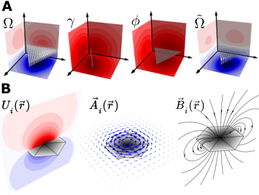
The first building block, used in all the field calculations, is the solid angle subtended at $\vec{r}$ by triangle $\Delta_{f}$ consisting of vertices $i$, $j$, and $k$: Van Oosterom and Strackee 1983

where $N=\vec{d}_{i}\times\vec{d}_{j}\cdot\vec{d}_{k}$ is the numerator and $D=|\vec{d}_{i}||\vec{d}_{j}||\vec{d}_{k}|+\sum_{l=(i,j,k)}|\vec{d}_{l}|(\vec{d}_{l+1}\cdot\vec{d}_{l-1})$ the denominator for the two-argument inverse tangent function $\mathrm{atan2}$ defined as in most standard programming languages. Here, $\vec{d}_{i}=\vec{r}-\vec{r}_{i}$ is a vector pointing from the vertex $i$ to the evaluation point $\vec{r}$ (see Fig. 1B). The magnetic scalar potential of unit (magnetic) dipole density on a triangle can be computed using the solid angle as $-\Omega_{f}/(4\pi)$.

The second building block is the potential of a line charge. The potential of a unit line charge on edge $\vec{e}_{i}$ (Fig. 1B) can be obtained as De Munck 1992

where $\vec{r}_{j}$ and $\vec{r}_{k}$ are the two ends of the edge $\vec{e}_{i}$.

With the two integrals above, we can express the potential of a unit charge density on a triangle $\Delta_{f}$: Ferguson, Zhang, and Stroink 1994

Here, $d_{f}=\hat{n}_{f}\cdot\vec{d}_{l+1}$ is the signed distance from the triangle plane along the plane normal and $x_{l}=\vec{G}_{f,l}\cdot\vec{d}_{l+1}$ is the normalized signed distance from the line extended from the edge $\vec{e}_{l}$ along $\vec{G}_{f,l}$ such that $x_{l}(\vec{r}_{l})=1$. The geometry related to these distances can be found in Fig. 1C.

Finally, we present the potential of a linearly varying dipolar density $h_{i}(\vec{r})$ on a triangle $\Delta_{f}$: De Munck 1992

where $c_{i,l}=\vec{e_{i}}\cdot\vec{e_{l}}/(2A_{f})$. As the notation in Eqs. (25) and (26) differ from the literature, we provide alternative, concise derivations of the formulas in Appendix B using the notation of this work.

The magnetic field $\vec{B}_{i}(\vec{r})$ of a constant current density in a triangle is derived in B and, using that result, the magnetic field due to a single hat-function current becomes

where $\mathcal{N}_{i}$ denotes the set of triangles neighbouring vertex $i$ as shown in Fig. 2. A corresponding formula expressed in local coordinates of a triangle has been derived by Pissanetzky. Pissanetzky 1992

The vector and scalar potentials for the current of a hat stream function $h_{i}$ can be obtained in a straightforward manner using the integrals in Sec. III.3. The vector potential [Eq. (5)] can be expressed using the discrete rotated-gradient [Eq.  (19)] and the integral $\phi_{f}(\vec{r})$: [Eq. (25)] Pissanetzky 1992; Koponen et al. 2017

The scalar potential [Eq. (6)] of $h_{i}$ involves only the potentials of linearly varying dipole densities $\tilde{\Omega}_{f,i}(\vec{r})$ [Eq. (26)]

The magnetic field and potentials due to a single hat-function current are illustrated in Fig. 3B.

In this basis, the mutual inductance operator $\boldsymbol{M}$ can also be interpreted as a mapping from the discretized stream function $\boldsymbol{s}$ to the magnetic flux (integrated normal component) at the mesh vertices. This can be seen from the second identity in Eq. (9): by replacing $\vec{m}_{k}$ with the dipole density $\hat{n}h_{k}$, the matrix element $M_{k,l}$ corresponds to the normal magnetic field of current $l$ integrated over the hat function of vertex $k$.

For mutual resistance we also have to model the surface conductivity $\sigma_{\mathrm{s}}$. Assuming piecewise-constant surface conductivity on the triangles, and using Eq. (10), we obtain the mutual resistance operator as

where $\sigma_{1}$ and $\sigma_{2}$ are the conductivities in triangles 1 and 2 neighbouring the edge from vertex $i$ to vertex $j$ (see Fig. 2). When $\sigma$ is constant over the surface, the resistance operator is proportional to the discrete surface Laplacian $R_{i,j}=-\frac{1}{\sigma_{\mathrm{s}}}L_{i,j}\,$. Several studies Lemdiasov and Ludwig 2005; Poole 2007; Lopez et al. 2009 use mutual resistance in this form although the relation to the discrete Laplacian has not been noted.

We obtain the expansion for the magnetic field by taking the gradient of the scalar potential:

where $\vec{V}_{lm}=(-(l+1)Y_{lm}\hat{r}+\nabla_{1}Y_{lm})/\sqrt{(l+1)(2l+1)}$ and $\vec{W}_{lm}=(lY_{lm}\hat{r}+\nabla_{1}Y_{lm})/\sqrt{l(2l+1)}$ are vector spherical harmonics. Hill 1954; Taulu and Kajola 2005 Here, $\nabla_{1}$ is the angular part of the gradient on a unit sphere. Plattner and Simons 2014 Both the set of vector spherical harmonics $\vec{V}_{lm}$, $\vec{W}_{lm}$, and the set of tangential vector spherical harmonics $\vec{X}_{lm}=-\hat{r}\times\nabla_{1}Y_{lm}/\sqrt{l(l+1)}$ are also orthonormal with respect to an inner product $\int_{\Omega}\vec{f}_{lm}\cdot\vec{g}_{l^{\prime}m^{\prime}}d\Omega\,$.

Because the multipole expansion of $\vec{B}$ is linear with respect to the coefficients, we can express it using linear operators $\boldsymbol{\vec{B}}_{\alpha}$ and $\boldsymbol{\vec{B}}_{\beta}$ as

where the expansions coefficients, truncated at a certain degree $l$, are stacked in the column vectors $\boldsymbol{\alpha}$ and $\boldsymbol{\beta}$. When the magnetic field is evaluated at a specific set of evaluation points, the linear operators above can be expressed as coupling matrices that map the given multipole coefficients to field values at the evaluation points.

The coefficients $\alpha_{lm}$ and $\beta_{lm}$ can be calculated directly from any surface-current distribution $\vec{j}(\vec{r})$ with help of the tangential vector spherical harmonics $\vec{X}_{lm}$ as Gray 1978; Nieminen et al. 2011

Using these equations together with the stream function in Eq. (1) and its discretization in Eq. (12), we define mesh operators (matrices) $\boldsymbol{C}_{\alpha}$ and $\boldsymbol{C}_{\beta}$ that map the stream-function values to the spherical harmonic coefficients

The convergence of the multipole series may be analyzed by inserting, for example, the inner multipole coefficients of Eq. (35) into Eq. (32) which yields terms involving factors $(r^{\prime}/r)^{(l-1)}$. If there are any sources with radius $r^{\prime}$ greater than the radius of the field point $r$, the factors $(r^{\prime}/r)^{(l-1)}$ approach infinity with growing $l$ and the series fails to converge. A similar analysis can be made for the outer sources. These analyses result in convergence regions for the expansions shown in Fig. 4A. As the figures show, the choice of the origin is crucial for the convergence, but it cannot be chosen in such a way that the series would converge everywhere in the volume where the scalar potential is defined.

We base the expansion on the eigenfunctions of the (negative) surface Laplacian. These eigenfunctions generalize a sinusoidal function basis, such as the spherical harmonics basis, to an arbitrary surface (see Fig. 5). Generally, these functions are characterized by the eigenvalue equation Levy 2006; Reuter et al. 2009

where the eigenvalue $k_{n}^{2}$ corresponds to the squared spatial frequency of the $n^{\mathrm{th}}$ eigenfunction $v_{n}$. The higher the order $n$ is, the higher the spatial frequency and the more zero crossings $v_{n}(\vec{r})$ has (Fig. 5). In relation to spherical harmonics, we call these functions surface harmonics (SUHs). In geometry processing, they are also known as manifold harmonics. Vallet and Lévy 2008

For practical computations, we discretize the functions as $v_{n}(\vec{r})=\sum_{i}V_{i,n}h_{i}(\vec{r})$, which leads to a discrete (generalized) eigenvalue equation Reuter et al. 2009

where $\boldsymbol{L}$ is the Laplace operator in Eq. (21) and $\boldsymbol{N}$ is a mass matrix taking into account the overlap of hat functions, and $\boldsymbol{v}_{n}$ correspond to columns of the matrix $\mathbf{V}$. As both $\boldsymbol{L}$ and $\boldsymbol{N}$ are sparse matrices, the vertex coefficient vectors $\boldsymbol{v}_{n}$ can be solved efficiently with sparse solvers. The resulting eigenfunctions $v_{n}(\vec{r})$ are orthonormal with respect to integration over the surface, which can be expressed in the discrete form as $\boldsymbol{v}_{n}^{\top}\boldsymbol{N}\boldsymbol{v}_{m}=\delta_{n,m}$.

Substituting the surface-harmonics representation of a stream function $\psi(\vec{r})=\sum_{n}a_{n}v_{n}(\vec{r})$ to Eq. (6), we can write the magnetic scalar potential as

Similarly, the SUH coefficients $\boldsymbol{a}$ can be mapped to the magnetic field as

Examples of the scalar potentials of the basis functions $v_{n}$ (SUH) are displayed in Fig. 4B with a comparison to the multipole expansion (SPH). Compared to the multipole potentials, in the SUH expansion, the potentials are distributed more uniformly around the corresponding surface.

The SUH expansion is not restricted to closed surfaces, but can be applied for stream functions on surfaces with boundaries and any number of holes. Such bases can be used for surface-coil design to decrease the degrees of freedom when optimizing surface currents, as demonstrated in the accompanying paper. Zetter et al. 2020

Instead of orthogonal stream functions, one may desire orthogonality in their magnetic fields. In that case, the basis functions can be solved from an discrete eigenvalue equation similar to Eq. (40) by replacing the mass matrix $\boldsymbol{N}$ with the inductance matrix $\boldsymbol{M}$. To enable physical interpretations, $\boldsymbol{L}$ can be replaced by $\boldsymbol{R}=\boldsymbol{L}/\sigma_{\mathrm{s}}$ to get the following eigenvalue equation

This equation is related to the independent modes of eddy currents on the conducting surface; $\tau_{n}$ is the time constant of the $n$th mode. These modes can be used, for example, to calculate the time dynamics of eddy-current induced fields Zevenhoven et al. 2014 or uncoupled current patterns for thermal noise calculations. Roth 1998; Iivanainen et al. 2020 It should be noted, however, that $\boldsymbol{M}$ is now a dense matrix, whereas $\boldsymbol{N}$ was very sparse, disabling the use of sparse eigensolvers and increasing computation time when building the matrix.

Let us consider a closed surface, inside which a desired field pattern is to be designed and a second (outer) surface, the exterior of which is to be shielded from the field. To derive a set of equations with a unique solution, we again discretize the surfaces using triangle meshes. The shielded field pattern can be obtained by designing suitable stream functions $\boldsymbol{s}_{1}$ and $\boldsymbol{s}_{2}$ on the two surfaces so that their combined field satisfies desired boundary conditions. Based on the discussion in Sec. III.5, we can write the boundary conditions for the normal component of the field at the surfaces using stacked mutual-inductance matrices $\boldsymbol{M}_{ij}$ as

where the first row corresponds to the desired magnetic field $\boldsymbol{b}_{\mathrm{n}}$ at the inner surface and the second row corresponds to the zero condition for the outer surface. Because $\boldsymbol{s}^{\top}\boldsymbol{M}\boldsymbol{s}$ is the total magnetic-field energy of the system, $\boldsymbol{M}$ is a positive semi-definite matrix. As the only zero eigenvalue is the one corresponding to a constant stream function (zero current), the system can be solved by inverting $\boldsymbol{M}$ deflated for the constant vector.

Two examples demonstrating the perfect shielding obtained by solving Eq. (44) are shown Fig. 6. The shielding by the outer surface corresponds to the situation where the exterior volume would be a superconductor that expels all fields so that no magnetic field crosses the outer surface. This is also analogous to an electrical volume-conductor problem where the exterior volume is insulating, confining the 3D current density.

When the outer current surface contains current-free regions in it, perfect cancellation of the primary field is generally not possible due to a lack of degrees of freedom in the current-pattern design. Next, we demonstrate a method to optimize the primary and shielding currents applicable also to an open surface geometry.

We will now optimize the primary current $\boldsymbol{s}_{1}$ for minimal energy with an additional constraint. Instead of a hard equality constraint for the desired field, we modify the cost function with a term that penalizes for the residual in desired multipole moments $\boldsymbol{\beta}$:

where $\lambda$ is a trade-off parameter between a perfect multipole fit and a minimal field energy. The coupling matrix $\boldsymbol{C}_{\beta}=\boldsymbol{C}_{\beta,1}+\boldsymbol{C}_{\beta,2}\boldsymbol{M}_{22}^{-1}\boldsymbol{M}_{21}$ is obtained using the constraint in Eq. (46); $\boldsymbol{C}_{\beta,i}$ are matrices that map $\boldsymbol{s}_{i}$ to the multipole moments. The solution for $\boldsymbol{s}_{1}$ that minimizes the cost function can again be found by equating the gradient $\nabla_{\boldsymbol{s_{1}}}E(\boldsymbol{s}_{1})$ to zero:

Examples of shielded configurations generated using the method above are shown in Fig. 7. Compared to the fields in Fig. 6, which are solved for a closed geometry, these fields leak in the directions where the shielding surface is missing. Thus, the placement of the shielding surfaces is crucial for the self-shielding performance.

Let us consider a primary potential $\boldsymbol{U}_{\mathrm{p}}(\vec{r})^{\top}\boldsymbol{s}_{\mathrm{p}}$ generated by a surface current with (discretized) stream function $\boldsymbol{s}_{\mathrm{p}}$ inside the magnetic shield. We can satisfy the equipotential condition on the shield by placing a suitable equivalent surface current $\boldsymbol{s}_{\mathrm{eq}}$ on the shield surface. In other words, we require that $\boldsymbol{U}_{\mathrm{p}}^{\top}(\vec{r})\boldsymbol{s}_{\mathrm{p}}+\boldsymbol{U}_{\mathrm{eq}}(\vec{r})^{\top}\boldsymbol{s}_{\mathrm{eq}}=0$ holds on the shield. To solve for $\boldsymbol{s}_{\mathrm{eq}}$, we apply the condition at collocation points on the shield mesh. Because $\boldsymbol{U}_{\mathrm{eq}}(\vec{r})\boldsymbol{s}_{\mathrm{eq}}$ is discontinuous across the shield, we apply the condition at collocation points slightly inwards from the shield surface as $\vec{r_{j}}-\epsilon\hat{n}_{j}$, where $\vec{r}_{j}$ are the vertex positions of the shield mesh, $\epsilon$ is a small number compared to the mesh resolution and $\vec{n}_{j}$ are the vertex normal vectors. After solving the resulting set of linear equations for $\boldsymbol{s}_{\mathrm{eq}}$, we can estimate the effect of the shield by $\boldsymbol{U}_{\mathrm{eq}}(\vec{r})^{\top}\boldsymbol{s}_{\mathrm{eq}}$ at all points inside the shield.

Figure 8 shows an example of a magnetically shielded configuration with a surface-current pattern on a bi-planar surface inside a perfect cylindrical magnetic shield. The current patterns on the planes are designed such that the field in the target volume, indicated by the dashed circle, is as homogeneous as possible. The secondary field due to the shield amplifies the magnetic field (the gradient of the potential) in the vicinity of the shield outside the target volume. The contribution from the cylinder cap also produces minor inhomogeneity in the magnetic field inside the target volume.

References

- Merkel (1987) P. Merkel, Nuclear Fusion 27, 867 (1987).
- Drevlak (1998) M. Drevlak, Fusion Technology 33, 106 (1998).
- Abe et al. (2003) M. Abe, T. Nakayama, S. Okamura, and K. Matsuoka, Physics of Plasmas 10, 1022 (2003).
- Pissanetzky (1992) S. Pissanetzky, Measurement Science and Technology 3, 667 (1992).
- Peeren (2003a) G. N. Peeren, Journal of Computational Physics 191, 305 (2003a).
- Lemdiasov and Ludwig (2005) R. A. Lemdiasov and R. Ludwig, Concepts in Magnetic Resonance Part B: Magnetic Resonance Engineering: An Educational Journal 26, 67 (2005).
- Poole (2007) M. S. Poole, Improved equipment and techniques for dynamic shimming in high field MRI, Ph.D. thesis, University of Nottingham (2007).
- Harris et al. (2013) C. T. Harris, D. W. Haw, W. B. Handler, and B. A. Chronik, Journal of Magnetic Resonance 234, 95 (2013).
- Hidalgo-Tobon (2010) S. Hidalgo-Tobon, Concepts in Magnetic Resonance Part A 36, 223 (2010).
- Koponen et al. (2017) L. M. Koponen, J. O. Nieminen, T. P. Mutanen, M. Stenroos, and R. J. Ilmoniemi, Brain stimulation 10, 795 (2017).
- Cobos Sánchez et al. (2018) C. Cobos Sánchez, F. J. Garcia-Pacheco, J. M. G. Rodriguez, and J. R. Hill, Engineering Analysis with Boundary Elements 88, 156 (2018).
- Bringout and Buzug (2014) G. Bringout and T. M. Buzug, IEEE Transactions on Magnetics 51, 1 (2014).
- Holmes et al. (2018) N. Holmes, J. Leggett, E. Boto, G. Roberts, R. M. Hill, T. M. Tierney, V. Shah, G. R. Barnes, M. J. Brookes, and R. Bowtell, NeuroImage 181, 760 (2018).
- Afach et al. (2014) S. Afach, G. Bison, K. Bodek, F. Burri, Z. Chowdhuri, M. Daum, M. Fertl, B. Franke, Z. Grujic, V. Hélaine, et al., Journal of Applied Physics 116, 084510 (2014).
- Wyszyński et al. (2017) G. Wyszyński, K. Bodek, S. Afach, G. Bison, Z. Chowdhuri, M. Daum, B. Franke, S. Komposch, B. Lauss, D. Ries, et al., AIP Advances 7, 035216 (2017).
- Roth and Wikswo Jr (1990) B. J. Roth and J. P. Wikswo Jr, Review of Scientific Instruments 61, 2439 (1990).
- Suits and Garroway (2003) B. Suits and A. Garroway, Journal of Applied Physics 94, 4170 (2003).
- Zevenhoven et al. (2014) K. C. J. Zevenhoven, S. Busch, M. Hatridge, F. Öisjöen, R. J. Ilmoniemi, and J. Clarke, Journal of Applied Physics 115, 1 (2014).
- Zevenhoven et al. (2015) K. C. J. Zevenhoven, H. Dong, R. J. Ilmoniemi, and J. Clarke, Applied Physics Letters 106, 034101 (2015).
- Roth (1998) B. J. Roth, Journal of Applied Physics 83, 635 (1998).
- Uhlemann et al. (2015) S. Uhlemann, H. Müller, J. Zach, and M. Haider, Ultramicroscopy 151, 199 (2015), special Issue: 80th Birthday of Harald Rose; PICO 2015 – Third Conference on Frontiers of Aberration Corrected Electron Microscopy.
- Vesanen et al. (2011) P. T. Vesanen, J. O. Nieminen, K. C. Zevenhoven, J. Dabek, J. Simola, J. Sarvas, and R. J. Ilmoniemi, IEEE Transactions on Magnetics 48, 53 (2011).
- Sumner, Pendlebury, and Smith (1987) T. J. Sumner, J. M. Pendlebury, and K. F. Smith, Journal of Physics D: Applied Physics 20, 1095 (1987).
- Blakely (1996) R. J. Blakely, Potential theory in gravity and magnetic applications (Cambridge University Press, 1996).
- Mendonca and Silva (1994) C. A. Mendonca and J. B. Silva, Geophysics 59, 722 (1994).
- Numminen et al. (1995) J. Numminen, S. Ahlfors, R. Ilmoniemi, J. Montonen, and J. Nenonen, IEEE Transactions on Biomedical Engineering 42, 72 (1995).
- Hänninen et al. (2001) H. Hänninen, P. Takala, M. Mäkijärvi, J. Montonen, P. Korhonen, L. Oikarinen, K. Simelius, J. Nenonen, T. Katila, and L. Toivonen, Basic research in cardiology 96, 405 (2001).
- Taulu and Kajola (2005) S. Taulu and M. Kajola, Journal of Applied Physics 97 (2005), 10.1063/1.1935742.
- Zetter et al. (2020) R. Zetter, A. J. Mäkinen, J. Iivanainen, K. C. J. Zevenhoven, R. J. Ilmoniemi, and L. Parkkonen, (2020), arXiv:2005.10056 [physics.comp-ph] .
- Turner (1986) R. Turner, Journal of Physics D: Applied Physics 19, L147 (1986).
- Crozier et al. (1995) S. Crozier, S. Dodd, K. Luescher, J. Field, and D. M. Doddrell, Magma: Magnetic Resonance Materials in Physics, Biology, and Medicine 3, 49 (1995).
- Brideson, Forbes, and Crozier (2002) M. A. Brideson, L. K. Forbes, and S. Crozier, Concepts in Magnetic Resonance: an Educational Journal 14, 9 (2002).
- Van Oosterom and Strackee (1983) A. Van Oosterom and J. Strackee, IEEE transactions on Biomedical Engineering , 125 (1983).
- De Munck (1992) J. De Munck, IEEE Transactions on Biomedical Engineering 39, 986 (1992).
- Ferguson, Zhang, and Stroink (1994) A. Ferguson, X. Zhang, and G. Stroink, IEEE Transactions on Biomedical Engineering 41, 455 (1994).
- de Goes, Desbrun, and Tong (2016) F. de Goes, M. Desbrun, and Y. Tong, in ACM SIGGRAPH 2016 Courses, SIGGRAPH ’16 (ACM, New York, NY, USA, 2016) pp. 27:1–27:49.
- Botsch et al. (2010) M. Botsch, L. Kobbelt, M. Pauly, P. Alliez, and B. Lévy, Polygon mesh processing (CRC press, 2010).
- Gray (1978) C. G. Gray, American Journal of Physics 46, 582 (1978).
- Nieminen et al. (2011) J. O. Nieminen, P. T. Vesanen, K. C. J. Zevenhoven, J. Dabek, J. Hassel, J. Luomahaara, J. S. Penttilä, and R. J. Ilmoniemi, Journal of Magnetic Resonance 212, 154 (2011).
- Levy (2006) B. Levy, in IEEE International Conference on Shape Modeling and Applications 2006 (SMI’06) (2006) pp. 13–13.
- Reuter et al. (2009) M. Reuter, S. Biasotti, D. Giorgi, G. Patanè, and M. Spagnuolo, Computers & Graphics 33, 381 (2009).
- Reusken (2020) A. Reusken, IMA Journal of Numerical Analysis 40, 109 (2020).
- Peeren (2003b) G. Peeren, Stream function approach for determining optimal surface currents, Ph.D. thesis, Philips Research (2003b).
- Lopez et al. (2009) H. S. Lopez, F. Liu, M. Poole, and S. Crozier, IEEE Transactions on Magnetics 45, 767 (2009).
- Jackson (1999) J. D. Jackson, Classical electrodynamics; 3rd ed. (John Wiley & Sons, Inc, New York, NY, 1999).
- Nédélec (2001) J.-C. Nédélec, Acoustic and electromagnetic equations: integral representations for harmonic problems (Springer-Verlag, 2001).
- Hackbusch (1995) W. Hackbusch, “Integral equations: Theory and numerical treatment,” (1995).
- Geselowitz (1967) D. B. Geselowitz, Biophysical journal 7, 1 (1967).
- MacNeal (1949) R. H. MacNeal, The solution of partial differential equations by means of electrical networks, Ph.D. thesis, California Institute of Technology (1949).
- Pinkall and Polthier (1993) U. Pinkall and K. Polthier, Experimental mathematics 2, 15 (1993).
- Jacobson (2013) A. Jacobson, Algorithms and interfaces for real-time deformation of 2d and 3d shapes, Ph.D. thesis, ETH Zurich (2013).
- Crane, Weischedel, and Wardetzky (2013) K. Crane, C. Weischedel, and M. Wardetzky, ACM Transactions on Graphics (TOG) 32, 1 (2013).
- Rao et al. (1979) S. Rao, A. Glisson, D. Wilton, and B. Vidula, IEEE Transactions on Antennas and Propagation 27, 604 (1979).
- Wilton et al. (1984) D. Wilton, S. Rao, A. Glisson, D. Schaubert, O. Al-Bundak, and C. Butler, IEEE Transactions on Antennas and Propagation 32, 276 (1984).
- Graglia (1993) R. D. Graglia, IEEE Transactions on Antennas and Propagation 41, 1448 (1993).
- Eibert and Hansen (1995) T. F. Eibert and V. Hansen, IEEE transactions on Antennas and Propagation 43, 1499 (1995).
- Xia et al. (2017) T. Xia, Z. Miao, S. Chen, H. Wang, and Y. Yao, PLOS ONE 12, 1 (2017).
- Plattner and Simons (2014) A. Plattner and F. J. Simons, Applied and Computational Harmonic Analysis 36, 1 (2014).
- Hill (1954) E. L. Hill, American Journal of Physics 22, 211 (1954).
- Vallet and Lévy (2008) B. Vallet and B. Lévy, in Computer Graphics Forum, Vol. 27 (Wiley Online Library, 2008) pp. 251–260.
- Iivanainen et al. (2020) J. Iivanainen, A. J. Mäkinen, R. Zetter, K. C. J. Zevenhoven, R. J. Ilmoniemi, and L. Parkkonen, in preparation (2020).
- Kybic et al. (2005) J. Kybic, M. Clerc, T. Abboud, O. Faugeras, R. Keriven, and T. Papadopoulo, IEEE transactions on Medical Imaging 24, 12 (2005).
- Stenroos, Mäntynen, and Nenonen (2007) M. Stenroos, V. Mäntynen, and J. Nenonen, Computer Methods and Programs in Biomedicine 88, 256 (2007).
- Sánchez et al. (2016) C. C. Sánchez, J. M. G. Rodriguez, Á. Q. Olozábal, and D. Blanco-Navarro, Physics in Medicine & Biology 62, 73 (2016).
- Wikswo and Swinney (1985) J. P. Wikswo and K. R. Swinney, Journal of Applied Physics 57, 4301 (1985).
- Nolte and Curio (1997) G. Nolte and G. Curio, Biophysical journal 73, 1253 (1997).
- Jerbi et al. (2002) K. Jerbi, J. C. Mosher, S. Baillet, and R. M. Leahy, Physics in Medicine & Biology 47, 523 (2002).
Appendix A Stream function as magnetic dipole density
In this appendix, we demonstrate the equivalence of the current-density and dipole-density interpretations of the stream function based on the magnetic vector potential. Let us start from the vector potential of a surface-current density: