Magnetic-field modeling with surface currents: Implementation and usage of bfieldtoolsPreprint: AIP/123-QED
Abstract
We present a novel open-source Python software package, bfieldtools, for magneto-quasistatic calculations with current densities on surfaces of arbitrary shape. The core functionality of the software relies on a stream-function representation of surface-current density and its discretization on a triangle mesh. Although this stream-function technique is well-known in certain fields, to date the related software implementations have not been published or have been limited to specific applications. With bfieldtools, we aimed to produce a general, easy-to-use and well-documented open-source software. The software package is written purely in Python; instead of explicitly using lower-level languages, we address computational bottlenecks through extensive vectorization and use of the NumPy library. The package enables easy deployment, rapid code development and facilitates application of the software to practical problems. In this paper, we describe the software package and give an extensive demonstration of its use with an emphasis on one of its main applications – coil design.
I Introduction
Within many fields of engineering and science, there is a need for modeling the relationship between magnetic fields and surface currents in complex geometries. For example, to model eddy currents in conducting sheets, one needs to calculate the coupling between the external field and the currents as well as the inductive effects of the currents within the conductor (Peeren 2003a; Zevenhoven et al. 2015, e.g.). Such modeling is also useful in computing the magnetic noise arising from thermal fluctuations (Roth 1998; Sandin et al. 2011; Iivanainen et al. 2020) and in designing surface-current patterns that generate a desired magnetic field. Finally, through such field calculations, surface currents can be used as equivalent sources in reconstruction and interpolation of magnetic fields, e.g., in geo- (Mendonça and Silva 1994; Blakely 1996) and biomagnetism (Taulu and Kajola 2005).
A current density is often represented using a set of basis functions. For currents on simple domains (such as planes, cylinders, toroids, or spheres), basis functions can be formed analytically (Turner 1986; Merkel 1987; Crozier et al. 1995; Liu and Petropoulos 1997; Drevlak 1998; Roth 1998; Suits and Garroway 2003; Forbes and Crozier 2004; Zevenhoven et al. 2014, e.g.). Pissanetzky 1992 introduced a general stream-function representation of the surface-current density on arbitrary surfaces, which discretizes the current on triangle surface meshes in a manner similar to finite-element and boundary-element methods (FEM and BEM, respectively).
Within the field of magnetic resonance imaging (MRI), triangle mesh -based stream-function methods have been applied to magnetic field modeling and coil design since the early 1990s (Pissanetzky 1992; Peeren 2003a; Lemdiasov and Ludwig 2005; Poole 2007; Harris et al. 2013, e.g.). Similar methods have also been used in plasma physics (Abe et al. 2003). More recently, the same principles have been used in the design of coils for transcranial magnetic stimulation (TMS) (Koponen et al. 2017; Cobos Sánchez et al. 2018) as well as magnetic nanoparticle imaging (Bringout, Grafe, and Buzug 2015).
Still, these coil-design techniques and surface-current models have most often been applied to simple geometries and their implementations have not been available for wider audiences. While the basic equations or concepts may be well-known, implementing, testing and validating such software requires considerable time and effort, something that may not be available for all prospective users.
In this paper, we present a novel open-source Python software package for magnetic field modeling and coil design, bfieldtools (available at https://bfieldtools.github.io). This paper focuses on describing the software package itself and demonstrates its usage through several examples. While we give a brief overview of the working principles behind the software in the following section, for a more thorough treatment of the underlying physics and computational aspects we refer to our accompanying publication (Mäkinen et al. 2020).
II Computations using the discrete stream function
bfieldtools uses the scalar stream-function representation of a surface current density (Pissanetzky 1992; Peeren 2003a), which is discretized as a piecewise linear function onto a triangle mesh. Compared to analytical methods that require certain symmetries for the source-current distributions, the use of triangle meshes as source domains provides the user with considerable geometrical freedom.
The triangle mesh discretization is based on approximating the stream functions linearly on the face of each triangle as in finite-element methods (FEM), and as illustrated in Fig. 1. A piecewise linear stream function is defined on the surface using so-called hat functions, which are defined as having the value one at a single vertex and falling linearly to zero at the edges of the triangles neighboring the vertex. The stream function can then be represented as a linear combination of the hat functions with weights
| (1) |
The stream function weights can be collected in a column vector . All operations in bfieldtools involving the stream function are linear, and can thus be represented as matrices operating on . For convenience, we will refer to as the stream function from here on.
The surface-current density is obtained as the rotated gradient (Mäkinen et al. 2020) of the piecewise linear stream function, which makes it constant on each triangle face. Thus, we can express the current density on the faces of the mesh as
| (2) |
where is the rotated gradient operator, which maps the scalar stream function defined on the mesh vertices to a 3-vector defined on the mesh faces. In Eq. 2, brackets are used to index individual elements of the operator. In practice, we represent the operators using multidimensional NumPy ndarrays, which are treated as a stack of 2D matrices, and with matrix multiplication applied with respect to their last two dimensions. Using ndarrays, Eq. 2 can be written in shorthand notation as
| (3) |
In this paper, we use bold lower- and upper-case symbols, e.g. and , to refer to column vectors and matrices, respectively.
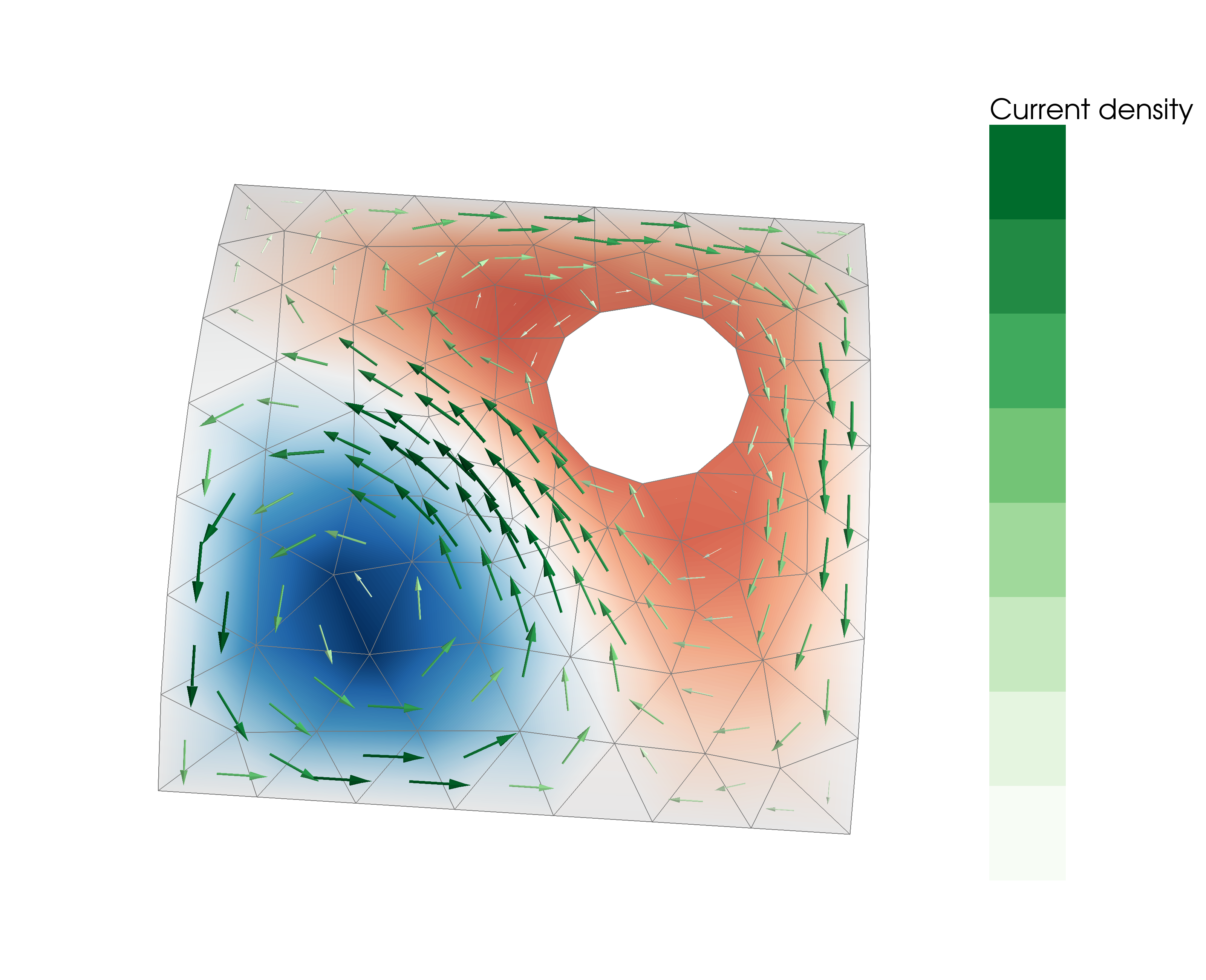
In the stream-function representation of surface-current density, the magnetic field and other related quantities (such as the magnetic potentials) at given points are linear functions of the stream function. For example, knowing the coupling between the stream function values defined at the vertices of the mesh and the magnetic field at the field evaluation points , the magnetic field at is computed as
| (4) |
Quantities related to energy can be obtained with quadratic expressions of the stream function. Using the inductance matrix [for definitions, see Mäkinen et al. 2020], the quadratic expression is the inductive field energy of the surface-current density. With the resistance matrix , the quadratic expression gives the Ohmic (heating) power of the surface current.
II.1 Stream-function optimization
When designing surface coils in the stream-function framework, one must find such an that fulfills the given requirements. The problem can be formulated as an optimization task. A requirement for minimal energy or power can be convenient since the optimization problem then becomes convex and thus has an unique solution which can be solved efficiently. Other requirements for can be included as inequality or equality constraints (e.g., one can constrain the magnetic field using Eq. 4), thus maintaining the convexity when the constraint equations are linear. A solution can be found as long as the set of constraints defines a non-empty set of candidate solutions. Coil design is discussed in more detail in Section IV.
II.2 Representations of fields and currents
In bfieldtools, the most flexible choice of basis for the stream function on a triangle mesh is arguably the direct use of the hat function basis, in which the surface current around each mesh vertex is described independently. Alternatively, one can apply the eigenfunctions of the surface Laplacian (Levy 2006; Reuter et al. 2009), which we call surface harmonics (SUH; Fig. 2; Mäkinen et al. 2020). The surface harmonics can be seen as a generalization of the more well-known spatial-frequency representations: on a sphere, the surface harmonics are essentially the spherical harmonics, and on a 2D plane, they correspond to the 2D Fourier series (Levy 2006). The series can represent smoothly-varying functions with a fairly small number of components, allowing the series to be truncated at a low order. For example, a stream function defined by the values on the 2000 vertices of a mesh might be expressed to a sufficient accuracy by 100 coefficients of the SUH series. Due to this compression, one can increase the mesh resolution without increasing the number of degrees of freedom and the computational cost, e.g., in optimization tasks. Truncating the SUH series also acts as an intuitive way to limit the maximum spatial frequency of the stream function and thereby in effect also its spatial gradient.

The surface harmonics are computed numerically using the generalized eigenvalue equation of the discretized surface-Laplacian operator (Levy 2006; Reuter et al. 2009)
| (5) |
where is a mass matrix taking into account the piecewise linear discretization of the mesh and contains the eigenvalues corresponding to the squared spatial frequencies of the surface harmonics, which are given by the columns of the basis matrix .
The SUH representation of a stream function can be obtained using the basis matrix as . Correspondingly, the magnetic field (Eq. 4) can be computed directly from :
| (6) |
Thus, the SUH coefficients can be used to specify any field that can be produced by a surface current on the corresponding surface mesh.
Another way to represent the magnetic field is the spherical multipole series (Taulu and Kajola 2005). In this representation, the coefficients and of the series can be used to specify the field in a source-free volume. The coefficients can be computed directly from the stream function with a linear mapping (Mäkinen et al. 2020)
| (7) |
where and are the coupling of the stream function to the coefficient vectors and , respectively, containing the multipole coefficients indexed linearly with increasing and up to a predefined cutoff. As in Eq. 6, these coefficients can also be linearly mapped to the magnetic field as
| (8) |
where and are the magnetic field coupling matrices representing spherical harmonic field components at the field evaluation points. This representation of the magnetic field is very compact for typical field profiles such as homogeneous or elementary gradient fields (which can be expressed with a single multipole coefficient), and can readily be applied, e.g., in coil design. To use the multipole series, the origin of the sphere used in the expansion has to be specified.
The SUH and multipole series can both provide a compact representation of the field. However, as discussed by Mäkinen and colleagues (Mäkinen et al. 2020), they have different convergence properties. The SUH and multipole coefficients can be fit to data, after which the estimated coefficients can be used to reconstruct and interpolate the magnetic field in the source-free space. In bfieldtools, we call the squared coefficients (both SUH and multipole) the spectrum of the magnetic field.
II.3 Boundary conditions
For the stream function to represent a divergence-free surface current (without current flowing in or out of the mesh), the derivative of the stream function along the boundaries of the mesh must be zero. In other words, the stream function must be constant on the boundary. It is typically convenient to set its value on the outer boundary of the mesh to zero. When the mesh has inner boundaries, the stream function value for the vertices on each boundary should be equal (but not necessarily zero). To enforce this, the hat functions along an inner boundary are combined into a single basis function, the value of which is constant along the boundary.
II.4 Eddy currents
There are many ways to control eddy-current-induced fields in a region of interest when quickly switching the applied magnetic field (Peeren 2003a; Zevenhoven et al. 2014; Zevenhoven et al. 2015, e.g.). Here, we present a way to compute the secondary field caused by eddy currents induced in some nearby conductor due to a primary field generated by a current in a surface coil. For an idealized case where the current waveform is a (Heaviside) step function, the instantaneous induced magnetic field caused by the eddy currents within a region of interest at time point is (Peeren 2003b)
| (9) |
where is the magnetic field coupling matrix of the conductive object to the region of interest, is the mutual inductance matrix between the coil mesh and the conductor mesh, and is the self-inductance matrix of the conductor mesh. Matrices and are determined by the generalized eigenvalue problem
| (10) |
where is the resistance matrix of the conductor and are the time constants of the different eddy current modes corresponding to the columns of .
II.5 Magnetic shielding
High-permeability shields are often used to minimize the effect of ambient magnetic fields on sensitive systems or experiments. However, the shield also distorts any magnetic fields generated inside the shield. When the relative permeability of the shield is high, the effect of the shield can be approximated by the boundary condition that the magnetic scalar potential on the inner shield surface is constant (Mäkinen et al. 2020). We solve this boundary condition by setting the constant to zero and by introducing an equivalent stream function to the shield surface such that
| (11) |
where and are the magnetic scalar potential coupling matrices of the coil and the shield for collocation points slightly inside the mesh. With the equipotential boundary condition, the magnetic field expression takes the form
| (12) |
which allows for the effect of magnetic shielding to be computed for any surface-current density within the shield.
III Software overview
bfieldtools is implemented purely in Python and leverages a large number of packages and libraries within the open-source scientific Python community. We use the trimesh package (Dawson-Haggerty 2020) for all mesh-related functionality. For numerical operations and linear algebra, we use NumPy (Oliphant 2015) and SciPy (Oliphant 2007; Virtanen et al. 2020). Visualizations are generated using matplotlib (Hunter 2007) and mayavi (Ramachandran and Varoquaux 2011) in two and three dimensions, respectively. The quadpy package (Schlömer, Ancellin, and Arnold 2020) is used for quadrature scheme generation for numerical integration, and the CVXPY package (Diamond and Boyd 2016; Agrawal et al. 2018) is employed in coil optimization.
bfieldtools has extensive online documentation, generated using Sphinx (https://www.sphinx-doc.org). The documentation includes an API reference, a large number of application examples acting as tutorials as well as links to background literature.
III.1 Software components
In this section, we summarize the functionality of the individual software submodules in bfieldtools. A graphical overview of the relations of the submodules in the package and the general software architecture is shown in Fig. 3.
Mesh conductor class
A large portion of the user-facing functionality of bfieldtools is centered around the use of MeshConductor objects that encapsulate a Trimesh triangle mesh object. The MeshConductor wrapper adds properties and methods such as the surface stream function, inductance and resistance matrices as well as magnetic field and potential coupling matrices. These properties are implemented with lazy evaluation, i.e. they are computed only when needed. In addition, the computed coupling matrices are cached to minimize redundant computation. Since the stream function may be represented in several different bases, the MeshConductor object is implemented such that it can internally handle basis changes.
Integrals
This submodule forms the core of bfieldtools. Using the analytical integral equations implemented in this submodule, most physical quantities used in the software package can be computed without numerical quadratures, yielding better accuracy in the vicinity of the mesh. In a typical use case, these functions are not directly accessed. Instead, they are used as building blocks for the mesh operators in other submodules. For an in-depth description of the analytical integrals, see Mäkinen et al. 2020.
Mesh calculus
This submodule implements calculus functions for triangle meshes. These functions include the gradient and rotated gradient, which map a scalar field represented as vertex values to tangential vector fields represented as 3-vectors on the mesh faces. The submodule also contains surface divergence and curl functions, which map tangential vector values on the faces to scalar values on the vertices (Botsch et al. 2010; de Goes, Desbrun, and Tong 2016; Reusken 2018, for more details see e.g.). Based on the same framework, the surface-Laplacian (or Laplace–Beltrami) operator (acting on scalars and vector functions defined on the vertices) is also implemented. Due to the boundary conditions discussed in Section II.3, the dimensions of the Laplacian differ for closed and open surfaWe present a novel open-source Python software package, bfieldtools, for magneto-quasistatic calculations with current densities on surfaces of arbitrary shape. The core functionality of the software relies on a stream-function representation of surface-current density and its discretization on a triangle mesh. Although this stream-function technique is well-known, to date the related software implementations have not been published or have been limited to specific applications. With bfieldtools, we aimed to produce a general, easy-to-use and well-documented open-source software. The software package is written purely in Python; instead of explicitly using lower-level languages, we address computational bottlenecks through extensive vectorization and use of the NumPy library. The package enables easy deployment, rapid code development and facilitates application of the software to practical problems. In this paper, we describe the software package and give an extensive demonstration of its use with an emphasis on one of its main applications – coil design.ces as well as for surfaces with holes, where each hole corresponds to one free value in the system. The mesh calculus module also includes a function to compute the mesh mass matrix used, e.g., in Eq. 5.
Mesh magnetics
This submodule contains functions for computing the coupling matrices of the magnetic field, vector potential and scalar potential (, and , respectively) described in Section II. In order to trade time for memory usage, the functions in this submodule include an option to compute the matrices in serial chunks. Furthermore, one may compute the magnetic field either using analytic integrals or, to speed up the computation, using numerical quadratures. When using the quadrature implementation, the choice of quadrature scheme can be freely specified by the user.
Mesh impedance
This submodule includes computations of, e.g., the resistance matrix , the (self-)inductance matrix , the mutual inductance matrix between two meshes as well as the mutual inductance between a mesh and loops of line currents (represented with connected current segments; see the line magnetics submodule). The inductance matrices are computed using the magnetic vector potential, as implemented in the mesh magnetics submodule. As these functions are highly vectorized, they are fast but require a significant amount of memory. As with the coupling matrix functions, the inductance matrix computations can be computed in serial chunks to save memory. Furthermore, one may speed up the computation by applying a numerical quadrature for evaluation points further away than a user-specified number of average triangle side lengths.
Contouring
For surface coil design, the contouring submodule contains functions for extracting discrete current loops from the continuous surface current density. The submodule also contains functions to process and smooth these current loops.
Line magnetics
bfieldtools includes a module for computations related to polyline currents comprising connected line segments. This includes the generated magnetic field as well as magnetic vector and scalar potentials. In addition, the module provides functions for computing (mutual) inductance of current loops.
Visualization
This submodule contains a variety of functions for visualizing meshes, stream functions, current loops, as well as fields and potentials. These functions are mainly wrappers for matplotlib (2D) and mayavi (3D) with suitable defaults for the type of data being plotted.
Spherical harmonics
bfieldtools includes a submodule containing functions for generating real (vector) spherical harmonics of arbitrary order as well as functions for multipole representation of the magnetic field (Eq. 8). Additionally, functions to, e.g., visualize the spherical harmonics, to estimate the spherical harmonics coefficients from data and to compute the multipole coefficients from the mesh stream function (Eq. 7) are provided. Different normalization schemes for the coefficients are provided.
Surface harmonics
The surface harmonics submodule contains tools for generating SUH components on a surface as well as working with SUH function expansions. These features are implemented in a class that calculates the expansion truncated to a given number of components. The returned object can be used for calculating the magnetic field associated with the SUH basis functions, estimating the SUH coefficients from data, as well for visualizing the functions.
Thermal noise
bfieldtools also includes a module for computing thermal AC magnetic noise arising from thin conducting objects (modeled using triangle meshes). The noise calculation implemented in the submodule uses the same computational stream-function framework and is described in more detail by Iivanainen et al. 2020.
Coil optimization
This submodule provides wrapper functions for quadratic coil optimization either using the regularized least-squares method or a numerical iterative solver via CVXPY. The functions take easy, human-readable parameters for the coil specification and constraints.
Utilities
Finally, bfieldtools includes a separate submodule for a variety of helper functions and utilities that are used across the other submodules.
IV Coil design
One of the main applications of the bieldtools software package is coil design. There are many applications in which one needs to design a coil fulfilling a set of requirements, e.g., on the field profile or homogeneity, the mechanical dimensions of the coil, stray field, coil heating and manufacturability. As discussed in Section II.1, the coils can be designed by optimizing a stream function such that a quadratic expression is minimized while some additional linear constraint(s) are met.
IV.1 Optimization methods
Depending on how the optimization problem is formulated, different optimization methods can be applied. In bfieldtools, the main optimization method for coil design is constrained quadratic optimization using a numerical iterative solver. The use of a numerical solvers allows the use of linear inequality constraints (such as allowing for a specific tolerance in, e.g., field profile). In bfieldtools, we employ the CVXPY convex optimization modeling language for accessible and easily applied optimization. When using CVXPY for optimizing the stream function , the problem statement is of the form
| (13) |
where is the quadratic objective matrix (e.g., inductance or resistance ), defines an optional linear penalty term, and the linear equality and inequality constraints are applied as needed. Multiple simultaneous constraints of the same type can easily be applied by stacking the constraint matrices. Furthermore, due to the flexibility of the CVXPY framework, one may also include additional constraints, such as constraining the -norm [e.g. 1-norm or -norm, as done by Poole and Jon Shah 2014] of a linear expression for , or by constraining the stream function value of specific vertices to be equal: .
An alternative approach (Pissanetzky 1992, e.g.) is to formulate the problem as a quadratic optimization without hard constraints, and instead use trade-off parameters. In this form, an example problem is formulated as
| (14) |
where determines the desired values of some quantity in some number of points and is the coupling matrix for that quantity and those points. Finally, is a scalar trade-off parameter, weighting the solution either towards minimizing the primary objective function or a penalty function. This formulation has a closed-form solution
| (15) |
which may be familiar as the Tikhonov-regularized least-squares formula. In the general case, multiple quadratic penalty terms may be applied, each with their own . In order to include linear equality constraints, one may, e.g., employ a Lagrange multiplier method as done by Lemdiasov and Ludwig 2005 and Poole 2007. However, while having good performance in problems with straightforward constraints, this inversion-based approach cannot accommodate hard inequality constraints.
IV.2 Objective functions
In bfieldtools, two main options for the quadratic objective are directly implemented. These are the minimization of the resistive power or the magnetic energy. Minimizing the resistive power results in a maximally smoothly varying stream function, as well as minimizing the resistive losses in the coil. This reduces the need for cooling the coil when large currents are used. Minimizing the magnetic energy results in minimal inductance of the coil. This reduces the voltage involved in fast ramping of the current in the coil.
Functions for magnetic and resistive energy minimization typically result in fairly similar stream functions. The two functions differ in that magnetic energy minimization allows for somewhat more variation at higher spatial frequencies of the stream function. These would be penalized more in resistive energy minimization. One may also form the quadratic objective as a weighted combination of resistive power and magnetic energy. Finally, bfieldtools allows for use of any other user-specified quadratic objective function.
IV.3 Constraints
Minimizing the quadratic objective without any penalty terms or constraints would lead to a trivial zero-current, zero-field solution. Thus, one must specify additional constraints to determine the final current pattern.
In coil design, constraining the magnetic field within a target region is the most typical constraint. In addition to specifying a target field one may also want to explicitly limit the stray field outside the coil. Using the spherical harmonics representation of the magnetic field as presented in Section II.2, one can also place constraints on and . Using a multipole-based constraint for the magnetic field naturally satisfies Maxwell’s equations in a source-free volume, whereas multiple user-specified point-based field constraints are not guaranteed to do so. One may also add other constraints, e.g. related to eddy currents (see Section II.4) or to high-permeability shielding (see Section II.5).
The use of inequality constraints in the optimization, as is possible when using an iterative solver, allows directly specifying the desired properties of the coil. This may be more intuitive than the use of trade-off/penalty parameters employed in the least-squares formulation. The use of inequality constraints also allows for wiggle room in the coil specification. This wiggle room decreases the need for apodization (Forbes and Crozier 2004; Hidalgo-Tobon 2010, e.g.), i.e. post-optimization smoothing of the stream function. Apodization has been applied due to high spatial-frequency oscillations or ’ringing’ in the stream function, which may arise when a target-field equality constraint is used, especially when minimizing the magnetic energy.
More sophisticated methods to limit high-frequency ringing directly constrain the gradient of the stream function; the spatial gradient of the stream function defines the surface-current density, and by extension, the spacing of the discretized coil windings. Constraining the maximum gradient affects the minimum spacing of windings, which can also be useful with regards to manufacturability. Limiting the maximum current density can also decrease local heating issues in high-power applications. The minimax method presented by Poole et al. 2010; Poole et al. 2012 should be similar in effect to constraining the stream function gradient, but works somewhat differently from an optimization viewpoint. An alternative way to reduce the minimum spacing of windings is to use a truncated SUH basis limited to low spatial frequencies.
IV.4 Discretization to wire segments
The surface-current density is obtained from the optimized stream function with Eq. 3. To extract the geometry of discrete conductor loops, one can simply use any number of stream function isolines with equal spacing in terms of stream function value. The number of isolines, i.e. current loops, can be freely chosen to fit the application; more loops will naturally result in a larger magnetic field per unit current and larger inductance, but will also better approximate the continuous surface current, thus having a smaller discretization error. Finally, the independent current loops must be connected in series, with special care taken to ensure that the current direction corresponds to the continuous current density. The manner in which the loops are connected should depend on manufacturing method and scale. For example, on a printed circuit board, the loops may be connected using vias and multiple layers, while larger-scale coils may even use soldered wire segments.
V Examples
The online documentation of bfieldtools (available at https://bfieldtools.github.io) contains several examples of applications, with code and accompanying explanatory text and figures. In this section, we discuss a number of selected examples in detail, walking through some of the software workflow, design decisions and rationale. However, for brevity and to focus on the essentials, we omit most imports as well as some repetitive or trivial steps. Online examples will be provided in full.
V.1 Biplanar coils with minimal stray field
In this example, we design a biplanar coil which produces homogeneous field within a spherical target region between the two square surface coils. In addition, we explicitly minimize the stray field on a spherical surface surrounding the coils. We start by importing the mesh file into a MeshConductor object. In this example, we use a very dense mesh, with 12 442 vertices and 24 304 faces. To speed up computation and limit the coil winding density, we use a truncated SUH representation for the stream function with .
We omit code lines for the generation of target and stray field points, and instead visualize the whole geometry in Fig. 4A. The target points are on a grid within a sphere around the centre of the biplanar coil (diameter 0.3 times the square side length), and the stray field points are on a spherical surface surrounding the coils (radius twice the square side length).

After having generated the geometry, we set the field specification at the defined target and stray points. In this case, we specify a homogeneous field along the -axis (within the target volume). We allow for <0.5% deviation in all three Cartesian components of the field at all target points. For all components of the stray field, we allow for <1% deviation from the target field amplitude. The homogeneous target field amplitude is set to a numerical value of for convenience. The absolute value does not matter, and will be scaled appropriately in the numerical solver. Having set the field specifications, we can run the numerical solver to optimize the stream function. We use the Ohmic power as the primary quadratic penalty and apply linear inequality constraints on the magnetic field at the target and stray field points.
Having computed the optimized stream function (see Fig. 4B), we can now convert the continuous stream function (current density) into discrete current loops and plot the result (as seen in Fig. 4C).
V.2 Eddy current minimization
Here, we use a geometry with a cylindrical coil surface similar to a conventional MRI bore, surrounded by a larger conducting cylindrical RF shield (both cylinder meshes have 4 764 vertices and 9 368 faces). We will design a reference coil which generates a homogeneous field along the X-axis (perpendicular to the long axis of the cylinder) within a spherical target volume. Furthermore, we will compute the eddy currents produced in the RF shield when switching the current in the coil. We also design another coil whose excitation generates minimal eddy-current field transients in the target volume. To this end, we add the expression in Eq. 9 as a constraint to the coil optimization procedure. We specifically do not use a an outer set of coils for self-shielding in order to showcase the eddy-current-induced field minimization procedure.
We omit the preparation steps shown in the previous example and instead present the geometry in Fig. 5. First, we compute the eddy-current modes and time constants of the cylindrical shield. As no current enters or leaves the shield, we set the stream function to zero at the boundary. The mesh boundary vertices are then not included in the generalized eigenvalue problem of Eq. 5 and the entries in corresponding to boundary vertices are fixed to zero by setting the MeshConductor object basis to ’inner’ (meaning inner vertices only). In this example, we only compute the 500 longest-lived eddy current modes, as the faster modes will have negligible effects past 1 ms.
Knowing the eddy-current dynamics, we can now define the coil-design specification and run the optimization procedure. In the static case, we allow for <0.5% field deviation on all field components from the target field at the target points. Additionally, we limit all components of the eddy-current-induced transient field at the target points at time points 1 ms, 3 ms and 5 ms to <5%, <1% and <0.25% of the homogeneous field strength, respectively.
First, for the reference coil, we omit the eddy-current-related parts of the coil specification. Then, for the second coil, we include the eddy-current constraints. The resulting discretized windings for the two coils are shown in Fig. 5A&B. In Fig. 5C, it is evident how much the eddy currents are suppressed for the second coil. The eddy-current field decays to below 1% of the static target field in 2.6 ms, whereas for the reference coil this time is 16.7 ms. Furthermore, Fig. 5D also shows the eddy-current pattern on the shield surface at different time points. For the coil in Fig. 5B, the eddy currents initially take such a pattern that they do not induce field in the target region. However, over time, the eddy-current pattern spreads and eventually resembles that of the reference coil in Fig. 5A, as the longer-lived eddy-current modes also have lower spatial frequencies.

V.3 Interactions with magnetic shielding
We consider the same square coil surfaces as in the first example, except now within a closed cylindrical magnetic shield (2 773 mesh vertices and 5 542 faces), see Fig. 6A. To emphasize the field distortion caused by the shield, we place the coils very close to the cylinder end. Again, we omit the preparations and only present the steps that lead to a coil in which the effect of the magnetic shielding is prospectively taken into account. We start by defining collocation points slightly inside the shield surface. We continue by solving Eq. 12, corresponding to the equipotential boundary condition at the shield (or at the collocation points). We include the solved field distortion in the coupling in the target field coupling matrix. In the optimization, we apply a linear inequality constraint for the target field.
The resulting coil windings are shown in Fig. 6C together with a reference coil design, for which the effect of the high-permeability shield was neglected (Fig. 6B). The field distribution within the target region is shown in Fig. 6D.

V.4 Magnetic field interpolation using equivalent surface currents
In this example, we represent a measured magnetic field using an equivalent surface current density. We use the equivalent current density to inter- and extrapolate the magnetic field in source-free space. Specifically, we apply the equivalent surface current representation to magnetoencephalography (MEG), in which the magnetic field produced by neural currents in the brain is measured using sensors positioned around the head. We use MEG data from the sample dataset of the MNE-Python software (Gramfort et al. 2014). The MEG data consists of measurements from 102 SQUID magnetometers sampled at 1 kHz during the presentation of repeated auditory beeps to the subject being measured. The magnetometers are oriented such that they measure the magnetic field component roughly normal to the subject’s scalp surface (see Fig. 7A).
We use the subject’s scalp surface (extracted from MR images) as the domain for the equivalent currents. Note that any surface that confines the “real” source currents generating the measured field would work. We use a regularized least-squares method to estimate the equivalent current distribution (corresponding to the stream function ) that attempts to reconstruct the measurements :
| (16) |
where the first term measures the norm of the current density over the surface with being the negative Laplacian operator (meaning that we assume the current density to be maximally smoothly varying), and the second term represents the residual between the measurements and the surface-current reconstruction. Here, is a coupling matrix that maps the stream function to the measured magnetic field component at the sensor positions and is a trade-off parameter to control the penalty on the residual in the reconstruction of the measurements.
To express the equivalent surface current in a compact manner, we apply a truncated surface-harmonic basis. The number of components is chosen such that it is large enough not to affect the result. For regularization, we use , where is the maximum eigenvalue of the matrix product .
Finally, using the estimated equivalent current density, we can compute the field at any point outside the scalp surface. The estimated surface stream function and its magnetic field reconstruction surrounding the head during the first peak of the auditory evoked response (–) is shown in Fig. 7A.

V.5 Field interpolation using spherical harmonics
In this example, we use the same data as in the previous example, but now we fit the data using spherical multipole components. We don’t utilize the scalp surface, but instead construct a multipole series with the origin at the approximate center of the sensor array. The inner expansion of the multipole series is bounded by a sphere that fits between the scalp surface and the sensor array. If all measurements are outside the inner expansion volume, and all active sources are within the volume, the -coefficients will determine the entire field Taulu and Kajola 2005.
We compute the fit for the inner expansion coefficients using the same regularized least-squares method as in the previous example (Eq. 16). We replace the scalp surface Laplacian by the surface Laplacian on a sphere. The regularization is set to , where is the maximum eigenvalue of the matrix product .
Having computed , we can now compute the magnetic field at any point in the outer expansion volume. A comparison between the magnetic field computed using the multipole series fit and the surface harmonics fit (Section V.4) at the sensor array surface can be seen in Fig. 7B. For comparison, the Figure also shows a 2D interpolation of the sensor data using multiquadric radial-basis functions, similar to the interpolation method used for visualizing MEG data in the MNE-Python software package (Gramfort et al. 2014).
VI Discussion
In this work, we have presented the features and different components of the bfieldtools software. Further, we have showcased its usage by several examples, including code snippets and visualizations.
VI.1 Software
Python has become a de-facto standard language for scientific software (Virtanen et al. 2020, see, e.g.,). We implemented bfieldtools in Python due to the rich open-source software ecosystem and large number of available libraries. In addition, Python allows for easy deployment of the software package across multiple platforms. Although the installation of the software depedencies is generally simple using official package installers (e.g. pip, https://pip.pypa.io/en/stable/) for the numerical solvers used in the coil optimization, the installation may include more complicated steps and vary across platforms.
We assume that the prospective users of bfieldtools are interested in understanding the details of the inner workings of the software. For that purpose, we strive to keep the software workflow straightforward and transparent by not hiding the NumPy arrays and other workings behind unnecessary layers of abstraction. For typical use, the MeshConductor class does include convenience functions and wrappers that reduce the need for explicit vertex indexing, function calls and extraneous variables. However, we also expose all intermediate and lower-level functions for advanced use and for, e.g, implementation of new functionality.
VI.2 Numerical operations and discretization
While bfieldtools does not include a meshing tool to create triangle surface meshes, most meshing tools used for finite-element modeling (FEM) or other physics modeling applications should produce meshes usable in bfieldtools. Typical FEM meshing rules of thumb also apply: the triangles should have small aspect ratios (preferably equilateral) and the mesh should have high enough resolution for the piecewise linear stream function to accurately represent the phenomena of interest. Narrow areas or areas close to mesh boundaries should generally have higher resolution.
When using functions employing quadrature approximation to compute, e.g., the magnetic field coupling matrix, the user is free to choose the quadrature scheme. In typical use, we recommend using a dense mesh with a low-order quadrature scheme, e.g. the centroid scheme, rather than using a sparse mesh with a high-order quadrature scheme. Quadrature schemes with points at the face corners or edges should be avoided, as they cause numerical issues due to singularities of the integrands.
When using CVXPY for (quadratic) optimization, the numerical solver backend can be chosen freely. Available solvers for quadratic programming include, e.g., MOSEK (Andersen and Andersen 2000), CVXOPT (Andersen, Dahl, and Vandenberghe 2019) and OSQP (Stellato et al. 2019). The examples in this work were run using MOSEK, which we have found to provide robust performance. However, MOSEK is a commercial product, and its use may thus be limited for some users, especially non-academic ones.
The solvers employed by CVXPY typically include (strict) feasibility checks in their optimization procedure. Additionally, they may specifically report which constraints are infeasible. The user thus gets immediate feedback on the physical feasibility of the design and can immediately respond, e.g., by altering the coil specification or the geometry.
VI.3 Performance
The examples in this paper were run on a regular workstation computer (4-core Intel Xeon E3-1230V5, 16 GiB RAM) with fairly dense meshes (2 000–12 000 vertices). The computation time of these examples was in the order of a one to a few minutes (biplanar coil example: 1 min 5 s; eddy current example: 5 min 49 s; magnetic shielding example: 6 min 43 s). Besides stream-function optimization, the most time-consuming part is generally the inductance matrix computation. For the self-inductance matrix, the computation time is roughly quadratic with respect to the number of mesh vertices with the approximate relation s (1 000 vertices: 7 s; 10 000 vertices: 868 s).
The use of surface harmonics speeds up many numerical operations such as the stream-function optimization. In the first example of this paper, instead of using the vertex-wise stream function representation with one degree of freedom for each of the 12 442 mesh vertices, we used a truncated SUH expansion with 100 degrees of freedom, which took 0.35 s for optimization and 3.7 s for constructing the SUH basis. By contrast, when optimizing vertex-wise, the solver ran out of memory (16 GiB) after 30 minutes. When using a more reasonably decimated mesh with 3 184 vertices and 6 076 faces, the vertex-wise stream-function optimization took 118 s.
VI.4 Outlook and future developments
In addition to the physical quantities and couplings described in Section II, there are other quantities for which linear mesh operators have been described previously, and which could also be implemented in bfieldtools. These include, e.g., torque due to a large (static) magnetic field (Lemdiasov and Ludwig 2005), temperature (Sánchez et al. 2015) and electric field in volume conductors (Koponen et al. 2017). These quantities are useful in specific applications and fields, e.g. torque is relevant in MRI coil design, and the electric field is especially important in TMS coil design.
The development of bfieldtools is ongoing. As the software is open source, we welcome users from the community to contribute to the development. With contributions from different fields of science and engineering, the scope of the software could be widened to new areas and use-cases.
Planned future work include the development of, e.g., dedicated data structures for different types of sensors and sensor arrays. We further strive to keep improving the software documentation and ease of access. The scope of the software could be readily extended to electric volume conductor problems in the form of the boundary-element method (BEM), where the existing integral implementations in bfieldtools can be applied.
VII Conclusion
We presented bfieldtools, a novel open-source software package for magnetic field modeling with surface currents. The backbone of the software is the stream-function representation of surface current on a triangle mesh. As a key feature, the software implements a flexible coil-design method applicable for a wide range of fields within physics and engineering. The release of bfieldtools as open source enables access to stream-function-based physics modeling with minimal effort.
Acknowledgments
This work has received funding from the European Union’s Horizon 2020 research and innovation programme under grant agreement No. 820393 (macQsimal), the European Research Council under ERC Grant Agreement no. 678578 (HRMEG), the Swedish Cultural Foundation under grant no. 140635 (author RZ), and by the Vilho, Yrjö and Kalle Väisälä Foundation (author AM).
Data availability
Data sharing is not applicable to this article as no new data were created or analyzed in this study.
References
References
- Abe et al. (2003) Abe, M., Nakayama, T., Okamura, S., and Matsuoka, K., Physics of Plasmas 10, 1022 (2003).
- Agrawal et al. (2018) Agrawal, A., Verschueren, R., Diamond, S., and Boyd, S., Journal of Control and Decision 5, 42 (2018).
- Andersen and Andersen (2000) Andersen, E. D. and Andersen, K. D., in High Performance Optimization, Applied Optimization, edited by H. Frenk, K. Roos, T. Terlaky, and S. Zhang (Springer US, Boston, MA, 2000) pp. 197–232.
- Andersen, Dahl, and Vandenberghe (2019) Andersen, M. S., Dahl, J., and Vandenberghe, L., “CVXOPT: A Python package for convex optimization,” (2019).
- Blakely (1996) Blakely, R. J., Potential Theory in Gravity and Magnetic Applications (Cambridge University Press, 1996).
- Botsch et al. (2010) Botsch, M., Kobbelt, L., Pauly, M., Alliez, P., and Lévy, B., Polygon mesh processing (CRC press, 2010).
- Bringout, Grafe, and Buzug (2015) Bringout, G., Grafe, K., and Buzug, T. M., IEEE Transactions on Magnetics 51, 1 (2015).
- Cobos Sánchez et al. (2018) Cobos Sánchez, C., Garcia-Pacheco, F. J., Rodriguez, J. M. G., and Hill, J. R., Engineering Analysis with Boundary Elements 88, 156 (2018).
- Crozier et al. (1995) Crozier, S., Dodd, S., Luescher, K., Field, J., and Doddrell, D. M., Magma: Magnetic Resonance Materials in Physics, Biology, and Medicine 3, 49 (1995).
- Dawson-Haggerty (2020) Dawson-Haggerty, M., “trimesh,” (2020).
- Diamond and Boyd (2016) Diamond, S. and Boyd, S., Journal of Machine Learning Research 17, 1 (2016).
- Drevlak (1998) Drevlak, M., Fusion Technology 33, 106 (1998).
- Forbes and Crozier (2004) Forbes, L. and Crozier, S., IEEE Transactions on Magnetics 40, 1929 (2004).
- de Goes, Desbrun, and Tong (2016) de Goes, F., Desbrun, M., and Tong, Y., in ACM SIGGRAPH 2016 Courses, SIGGRAPH ’16 (Association for Computing Machinery, Anaheim, California, 2016) pp. 1–49.
- Gramfort et al. (2014) Gramfort, A., Luessi, M., Larson, E., Engemann, D. A., Strohmeier, D., Brodbeck, C., Parkkonen, L., and Hämäläinen, M. S., NeuroImage 86, 446 (2014).
- Harris et al. (2013) Harris, C. T., Haw, D. W., Handler, W. B., and Chronik, B. A., Journal of Magnetic Resonance 234, 95 (2013).
- Hidalgo-Tobon (2010) Hidalgo-Tobon, S. S., Concepts in Magnetic Resonance Part A 36A, 223 (2010).
- Hunter (2007) Hunter, J. D., Computing in Science Engineering 9, 90 (2007).
- Iivanainen et al. (2020) Iivanainen, J., Mäkinen, A. J., Zetter, R., Zevenhoven, K. C. J., Ilmoniemi, R. J., and Parkkonen, L., in preparation (2020).
- Koponen et al. (2017) Koponen, L. M., Nieminen, J. O., Mutanen, T. P., Stenroos, M., and Ilmoniemi, R. J., Brain Stimulation 10, 795 (2017).
- Lemdiasov and Ludwig (2005) Lemdiasov, R. A. and Ludwig, R., Concepts in Magnetic Resonance Part B: Magnetic Resonance Engineering 26B, 67 (2005).
- Levy (2006) Levy, B., in IEEE International Conference on Shape Modeling and Applications 2006 (SMI’06) (IEEE, Matsushima, Japan, 2006) pp. 13–13.
- Liu and Petropoulos (1997) Liu, H. and Petropoulos, L. S., Journal of Applied Physics 81, 3853 (1997).
- Mendonça and Silva (1994) Mendonça, C. A. and Silva, J. B. C., GEOPHYSICS 59, 722 (1994).
- Merkel (1987) Merkel, P., Nuclear Fusion 27, 867 (1987).
- Mäkinen et al. (2020) Mäkinen, A. J., Zetter, R., Iivanainen, J., Zevenhoven, K. C. J., Parkkonen, L., and Ilmoniemi, R. J., arXiv (2020), 2005.10060 .
- Oliphant (2007) Oliphant, T. E., Computing in Science Engineering 9, 10 (2007).
- Oliphant (2015) Oliphant, T. E., Guide to NumPy, 2nd ed. (CreateSpace Independent Publishing Platform, USA, 2015).
- Peeren (2003a) Peeren, G. N., Stream Function Approach for Determining Optimal Surface Currents, Ph.D. thesis, Eindhoven University of Technology (2003a).
- Peeren (2003b) Peeren, G. N., Journal of Computational Physics 191, 305 (2003b).
- Pissanetzky (1992) Pissanetzky, S., Measurement Science and Technology 3, 667 (1992).
- Poole (2007) Poole, M., Improved Equipment and Techniques for Dynamic Shimming in High Field MRI, Ph.D. thesis, University of Nottingham (2007).
- Poole et al. (2010) Poole, M., Weiss, P., Lopez, H. S., Ng, M., and Crozier, S., Journal of Physics D: Applied Physics 43, 095001 (2010).
- Poole and Jon Shah (2014) Poole, M. S. and Jon Shah, N., Journal of Magnetic Resonance 244, 36 (2014).
- Poole et al. (2012) Poole, M. S., While, P. T., Lopez, H. S., and Crozier, S., Magnetic Resonance in Medicine 68, 639 (2012).
- Ramachandran and Varoquaux (2011) Ramachandran, P. and Varoquaux, G., Computing in Science Engineering 13, 40 (2011).
- Reusken (2018) Reusken, A., IMA Journal of Numerical Analysis 40, 109 (2018).
- Reuter et al. (2009) Reuter, M., Biasotti, S., Giorgi, D., Patanè, G., and Spagnuolo, M., Computers & Graphics IEEE International Conference on Shape Modelling and Applications 2009, 33, 381 (2009).
- Roth (1998) Roth, B. J., Journal of Applied Physics 83, 635 (1998).
- Sandin et al. (2011) Sandin, H. J., Volegov, P. L., Espy, M. A., Matlashov, A. N., Savukov, I. M., and Schultz, L. J., IEEE Transactions on Applied Superconductivity 21, 489 (2011).
- Schlömer, Ancellin, and Arnold (2020) Schlömer, N., Ancellin, M., and Arnold, D., Zenodo (2020), 10.5281/zenodo.1173132.
- Stellato et al. (2019) Stellato, B., Banjac, G., Goulart, P., Bemporad, A., and Boyd, S., arXiv (2019), 1711.08013 .
- Suits and Garroway (2003) Suits, B. H. and Garroway, A. N., Journal of Applied Physics 94, 4170 (2003).
- Sánchez et al. (2015) Sánchez, C. C., Rodriguez, J. M. G., Olozábal, Á. Q., and Poole, M., Engineering Analysis with Boundary Elements 59, 159 (2015).
- Taulu and Kajola (2005) Taulu, S. and Kajola, M., Journal of Applied Physics 97 (2005), 10.1063/1.1935742.
- Turner (1986) Turner, R., Journal of Physics D: Applied Physics 19, L147 (1986).
- Virtanen et al. (2020) Virtanen, P., Gommers, R., Oliphant, T. E., Haberland, M., Reddy, T., Cournapeau, D., Burovski, E., Peterson, P., Weckesser, W., Bright, J., Walt, S. J. v. d., Brett, M., Wilson, J., Millman, K. J., Mayorov, N., Nelson, A. R. J., Jones, E., Kern, R., Larson, E., Carey, C. J., Polat, I., Feng, Y., Moore, E. W., VanderPlas, J., Laxalde, D., Perktold, J., Cimrman, R., Henriksen, I., Quintero, E. A., Harris, C. R., Archibald, A. M., Ribeiro, A. H., Pedregosa, F., and Mulbregt, P. v., Nature Methods , 1 (2020).
- Zevenhoven et al. (2014) Zevenhoven, K. C. J., Busch, S., Hatridge, M., Öisjöen, F., Ilmoniemi, R. J., and Clarke, J., Journal of Applied Physics 115, 1 (2014).
- Zevenhoven et al. (2015) Zevenhoven, K. C. J., Dong, H., Ilmoniemi, R. J., and Clarke, J., Applied Physics Letters 106, 034101 (2015).