Plasmonically enhanced mid-IR light source based on tunable spectrally and directionally selective thermal emission from nanopatterned graphene

An object that is kept in equilibrium at a given temperature $T>0$ K emits electromagnetic (EM) radiation because the charge carriers on the atomic and molecular scale oscillate due to their heat energy.Baranov et al. 2019 Planck’s law describes quantitatively the energy density $u(\omega)$ of the EM radiation per unit frequency $\omega$ for black-body radiation, which is $u_{BB}(\omega)d\omega=\frac{\omega^{2}}{\pi^{2}c^{3}}\Theta(\omega)d\omega$, where $c$ is the speed of light in vacuum, $\hbar$ is the Planck constant, and $k_{B}$ is the Boltzmann constant. $\Theta(\omega,T)=\hbar\omega/[\exp(\hbar\omega/k_{B}T)-1]$ is the thermal energy of a photon mode. Consequently, the energy emitted per unit surface area and per unit frequency, also called spectral radiance, of a black body into three-dimensional (3D) space is given by

The total energy density $u$ can then be obtained by integrating over all frequencies and angles over the half-sphere, leading to the Stefan-Boltzmann law for the energy density of black-body radiation,

with $a_{BB}=7.566\times 10^{-16}$ Jm^-3K^-4. The total power emitted per unit surface area $P/A$ of a black-body is

where $b_{BB}=5.67\times 10^{-8}$ Wm^-2K^-4 is the Stefan-Boltzmann constant. The factor $\cos\theta$ is due to the fact that black bodies are Lambertian radiators.

In recent years, several methods have been implemented for achieving a spectrally selective emittance, in particular narrowband emittance, which increases the coherence of the emitted photons. One possibility is to use a material that exhibits optical resonances due to the band structure or due to confinement of the charge carriers.Baranov et al. 2019 Another method is to use structural optical resonances to enhance and/or suppress the emittance. Recently, photonic crystal structures have been used to implement passive pass band filters that reflect the thermal emission at wavelengths that match the photonic bandgap.Cornelius and Dowling 1999; Lin et al. 2000 Alternatively, a truncated photonic crystal can be used to enhance the emittance at resonant frequencies.Celanovic et al. 2005; Yang et al. 2017

Recent experiments have shown that it is possible to generate infrared (IR) emission by means of Joule heating created by means of a bias voltage applied to graphene on a SiO₂/Si substrate.Freitag et al. 2010; Luxmoore et al. 2013 In order to avoid the breakdown of the graphene sheet at around $T=700$ K, the graphene sheet can be encapsulated between hexagonal boron nitride (h-BN) layers, which remove efficiently the heat from graphene. The top layer protects it from oxidation.Kim et al. 2018; Luo et al. 2019 In this way, the graphene sheet can be heated up to $T=1600$ K,Luo et al. 2019 or even above $T=2000$ K.Kim et al. 2018; Shiue et al. 2019 Kim et al. and Luo et al. demonstrated broadband visible emission peaked around a wavelength of $\lambda=725$ nm.Kim et al. 2018; Luo et al. 2019 By using a photonic crystal substrate made of Si, Shiue et al. demonstrated narrowband near-IR emission peaked at around $\lambda=1600$ nm with an emittance of around $\epsilon=0.07$.Shiue et al. 2019 To the best of our knowledge, there are neither theoretical nor experimental studies on spectrally selective thermal emission from graphene in the mid-IR range.

Here, we present the proof of concept of a method to tune the spectrally selective thermal emission from nanopatterned graphene (NPG) by means of a gate voltage that varies the resonance wavelength of localized surface plasmons (LSPs) around the circular holes that are arranged in a hexagonal or square lattice pattern in a single graphene sheet in the wavelength regime between 3 $\mu$m and 12 $\mu$m. By generalizing Planck’s radiation theory to grey-body emission, we show that the thermal emission spectrum can be tuned in or out of the two main atmospheric transparency windows of 3 to 5 $\mu$m and 8 to 12 $\mu$m in the mid-IR regime, and also in or out of the opaque mid-IR regime between 5 and 8 $\mu$m. In addition, the gate voltage can be used to tune the direction of the thermal emission due to the coherence between the localized surface plasmons (LSPs) around the holes due to the nonlocal response function in graphene, which we show by means of a nonlocal fluctuation-dissipation theorem. The main element of the nanostructure is a circular hole of diameter $a$ in a graphene sheet. Therefore let us focus first on the optoelectronic properties of a single hole.

The frequency-dependent dipole moment of the hole is

where the polarizabilities $\alpha_{1,2}$ are given along the main axes $x$ and $y$ of the elliptic hole, and ${\bf r}={\bf r}_{0}$ is the position of the dipole moment, i.e. the hole. Graphene’s dielectric function is isotropic in the xy-plane, i.e. $\varepsilon^{\prime\prime}_{||}=\varepsilon^{\prime\prime}_{xx}=\varepsilon^{\prime\prime}_{yy}$. $V_{0}$ is the volume of the graphene sheet. In the Supplementary Information we derive the general polarizabilities of an uncharged single-sheet hyperboloid with dielectric function $\varepsilon(\omega)$ inside a medium with dielectric constant $\varepsilon_{m}$ [see Eq. (165)]. The polarizabilities of an elliptical wormhole in $x$- and $y$-direction read

respectively, for which the in-plane polarizabilities lies in the plane of the graphene sheet that is parallel to the $xy$-plane. $\varepsilon(\omega)$ is the dielectric function of graphene. We assumed that the thickness $d$ of the graphene sheet is much smaller than the size of the elliptic hole. The geometrical factors in this limit are

In the case of a circular hole of diameter $a$ the polarizability simplifies to

The localized surface plasmon resonance (LSP) frequency of the hole can be determined from the equation

the condition for which the denominator of $\alpha_{||}$ vanishes.

Using the linear dispersion relation, the intraband optical conductivity isSafaei et al. 2017; Paudel et al. 2017

which in the case of ${\varepsilon_{F}}\gg{k_{B}}T$ is reduced to

where $\tau$ is determined by impurity scattering and electron-phonon interaction ${\tau^{-1}}=\tau_{imp}^{-1}+\tau_{e-ph}^{-1}$ . Using the mobility $\mu$ of the NPG sheet, it can be presented in the form $\tau^{-1}=ev_{F}^{2}/(\mu E_{F})$, where $v_{F}=10^{6}$ m/s is the Fermi velocity in graphene. $\omega_{p}=\sqrt{e^{2}\epsilon_{F}/2\varepsilon_{m}}$ is the bulk graphene plasma frequency.

It is well-known by now that hydrodynamic effects play an important role in graphene because the Coulomb interaction collision rate is dominant, i.e. $\tau_{ee}^{-1}\gg\tau_{imp}^{-1}$ and $\tau_{ee}^{-1}\gg\tau_{e-ph}^{-1}$, which corresponds to the hydrodynamic regime. $\tau_{imp}^{-1}$ and $\tau_{e-ph}^{-1}$ are the electron-impurity and electron-phonon collision rates. Since for large absorbance and emittance, we choose a large Fermi energy, we are in the Fermi liquid regime of the graphene sheet. Taking the hydrodynamic correction into account, we also consider the hydrodynamically adjusted intraband optical conductivity,Bandurin et al. 2016; Christensen 2017

where $\eta^{2}=\beta^{2}+D^{2}\omega(\gamma+i\omega)$, $\beta^{2}\approx\frac{3}{4}v_{F}^{2}$ is the intraband pressure velocity, $D\approx 0.4$ $\mu$m is the diffusion length in graphene, and $\gamma=\tau^{-1}$ is the relaxation rate. Interestingly, the optical conductivity becomes $k$-dependent and nonlocal. Also, below we will conjecture that the diffusion length $D$ must be frequency-dependent.

Note that since $\varepsilon=1+\chi$, where $\chi$ is the susceptibility, it is possible to replace $\varepsilon^{\prime\prime}=\chi^{\prime\prime}$. Alternatively, using the formula of the polarizability $\alpha=\varepsilon_{0}\chi$ we can write $\varepsilon^{\prime\prime}=\alpha^{\prime\prime}/\varepsilon_{0}$. The dielectric function for graphene is given bySafaei et al. 2017; Paudel et al. 2017

where $\epsilon_{g}=2.5$ is the dielectric constant of graphite and $d$ is the thickness of graphene. Inserting this formula into Eq. (10) gives

Solving for the frequency and using the real part we obtain the LSP frequency,

which is linear in the Fermi energy $\epsilon_{F}$.

Let us now consider the 2D array of circular holes in a graphene sheet. Since the dipole moments $p_{j}=\delta{\bf p}({\bf R}_{j},\omega)$ interact with each other by inducing dipole moments, we need to consider the dressed dipole moment at each site ${\bf R}_{j}$ as source of the electric field, which is

where $\mathcal{G}_{jj^{\prime}}$ is the dipole-dipole interaction tensor. Using Bloch’s theorem $p_{j}=p_{0}\exp(i{\bf k}_{||}\cdot{\bf R}_{||})$, the effective dipole moment becomes

for each site $j$, and thus

The lattice some over the dipole-dipole interaction tensor $\mathcal{G}=\sum\limits_{j^{\prime}\neq j}\mathcal{G}_{jj^{\prime}}e^{i{\bf k}_{||}\cdot({\bf R}_{j}-{\bf R}_{j^{\prime}})}$ can be found in Ref. Thongrattanasiri et al. 2012, i.e.

where $\mathcal{P}$ is the lattice period,

$\Omega_{0}$ is the unit-cell area, and the real part is valid for periods much smaller than the wavelength. The factor $g=5.52$ ($g=4.52$) for hexagonal (square) lattice. The electric field created by the effective dipole moment is determined by

from which we obtain the effective polarizability of a hole in the coupled dipole approximation (CDA),

This formula is the same as in Refs. Zhao et al. 2003; Thongrattanasiri et al. 2012, where the absorption of electromagnetic waves by arrays of dipole moments and graphene disks were considered, respectively. Thus, our result corroborates Kirchhoff’s law (see below). Consequently, we obtain the same reflection and transmission amplitudes as in Ref. Thongrattanasiri et al. 2012, i.e.

where the upper (lower) sign and $S=2\pi\omega/c\Omega_{0}\cos\theta$ ($S=2\pi\omega\cos\theta/c\Omega_{0}$) apply to s (p) polarization. Thus, the emittance and absorbance of the bare NPG sheet are given by

The coupling to the interface of the substrate with reflection and transmission amplitudes $r_{0}$ and $t_{0}$, respectively, which is located basically at the same position as the NPG sheet, yields the combined reflection and transmission amplitudesThongrattanasiri et al. 2012

where $r^{\prime}=r$ and $t^{\prime}=1-r$ are the reflection and transmission amplitudes in backwards direction, respectively.

If we include also the whole substrate including cavity and Au mirror, we need to sum over all possible optical paths in the Fabry-Perot cavity, yielding

with

where $r_{Au}$ is the complex reflection amplitude of the Au mirror in the IR regime. $\delta=2kL\cos\theta$ is the phase accumulated by one back-and-forth scattering inside the Fabry-Perot cavity of length $L$. $k\approx n_{SU_{8}}k_{0}$ is the wavenumber inside the cavity for an external EM wave with wavenumber $k_{0}=2\pi/\lambda$. Since the sum is taken over a geometric series, we obtain

Since the transmission coefficient through the Au mirror can be neglected, we obtain the emittance $\epsilon$ and absorbance $A$ including cavity, i.e.

Using these results, let us consider the excitation of the graphene sheet near the hole by means of thermal fluctuations, which give rise to a fluctuating EM field of a localized surface plasmon (LSP). This can be best understood by means of the fluctuation-dissipation theorem, which provides a relation between the rate of energy dissipation in a non-equilibrium system and the quantum and thermal fluctuations occuring spontaneously at different times in an equilibrium system.Novotny and Hecht 2012 The standard (local) fluctuation-dissipation theorem for fluctuating currents $\delta\hat{J}_{\nu}({\bf r},\omega)$ in three dimensions reads

where the relative permittivity $\varepsilon({\bf r},\omega)=\varepsilon^{\prime}({\bf r},\omega)+i\varepsilon^{\prime\prime}({\bf r},\omega)=f({\bf r})\varepsilon(\omega)$ and $\mu,\nu=x,y,z$ are the coordinates. Note that since $\varepsilon=1+\chi$, where $\chi$ is the susceptibility, it is possible to replace $\varepsilon^{\prime\prime}=\chi^{\prime\prime}$. Alternatively, using the formula of the polarizability $\alpha=\varepsilon_{0}\chi$ we can write $\varepsilon^{\prime\prime}=\alpha^{\prime\prime}/\varepsilon_{0}$. $f({\bf r})=1$ on the graphene sheet and 0 otherwise. Since the fluctuating currents are contained inside the two-dimensional graphene sheet, we write the local fluctuation-dissipation theorem in its two-dimensional form, i.e.

where the fluctuating current densities have units of A/m² and the coordinates are in-plane of the graphene sheet.

Using the method of dyadic Green’s functions, it is possible to express the fluctuating electric field generated by the fluctuating current density by

where $\Omega$ is the surface of the graphene sheet. The LSP excitation around a hole can be well approximated by a dipole field such that

where ${\bf R}_{j}=(x_{j},y_{j})$ are the positions of the holes in the graphene sheet.

Consequently, we have

The dyadic Green function is defined as

with the scalar Green function given by

and ${\bf k}(\omega)^{2}=(\omega^{2}/c^{2})[\varepsilon_{xx}(\omega),\varepsilon_{yy}(\omega),\varepsilon_{zz}(\omega)]$.

Then, the fluctuation-dissipation theorem can be recast into the forms

and thus we obtain

noting that the dielectric tensor $\varepsilon^{\prime\prime}({\bf r},\omega)$ is diagonal.

Since the energy density of the emitted electric field at the point ${\bf r}$ is

we can write the spectral radiance as

assuming that the dipole current of the LSP is in the plane of the graphene sheet, i.e. the xy-plane, and the polarizability is isotropic, ie. ${\sigma^{\prime}}_{||}^{2D}={\sigma^{\prime}}_{xx}^{2D}={\sigma^{\prime}}_{yy}^{2D}$, and the same for all holes. $N$ is the number of holes. In order to obtain the spectral radiance in the far field, we need to integrate over the spherical angle. Using the results from the Supplementary Information, we obtain

where we used the definition of the absorbance of a 2D material, i.e.

with 2D complex conductivity $\sigma_{2D}(\omega)$. According to Kirchhoff’s law, emittance $\epsilon(\omega)$, absorbance $A(\omega)$, reflectance $R(\omega)$, and transmittance $T(\omega)$ are related byLifshitz and Pitaevskii 1980

from which we obtain the grey-body thermal emission formula

whose prefactor bears strong similarity to Planck’s black body formula in Eq. (1).

Using FDTD to calculate the emittance $\epsilon_{||}^{2D}(\omega)$, we evaluted the grey-body thermal emission according to Eq. (46) for the thermal emitter structure based on NPG shown in Figs. 1 and 2. Using COMSOL, we calculated the temperature distribution inside the NPG sheet, as shown in Fig. 8, when a bias voltage $V_{\rm SD}$ is applied, which gives rise to Joule heating. Our results are shown in Figs. 6, 7, and 9 for the temperatures $1300$ K, $1700$ K, and $2000$ K of NPG. After integrating over the wavelength under the curves, we obtain the following thermal emission power per area:

Let us consider the dependence of the thermal emission of NPG on the angle $\theta$. Integrating over $r^{2}\varphi$ we obtain

which is a clear deviation from a Lambert radiator. The pattern of the thermal radiation can be determined by

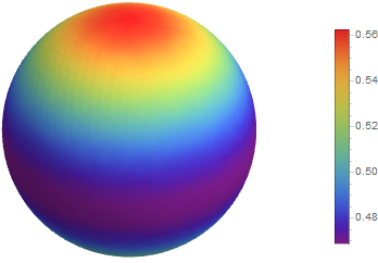
which is shown in Fig. 10. Interestingly, since we assumed that thermal emission is completely incoherent [see Eq. (42)] the thermal emission from NPG is only weakly dependent on the emission angle $\theta$, which can be clearly seen in Fig. 10.

However, the assumption that thermal emission of radiation is incoherent is not always true. Since Kirchhoff’s law is valid, thermal sources can be coherent.Greffet 2017 After theoretical calculations predicted that long-range coherence may exist for thermal emission in the case of resonant surface waves, either plasmonic or phononic in nature,Carminati and Greffet 1999; Henkel et al. 2000 experiments showed that a periodic microstructure in the polar material SiC exhibits coherence over many wavelengths and radiates in well-defined and controlled directions.Greffet et al. 2002 Here we show that the coherence length of a graphene sheet patterned with circular holes can be as large as 150 $\mu$m due to the plasmonic wave in the graphene sheet, thereby paving the way for the creation of phased arrays made of nanoantennas represented by the holes in NPG.

The coherence of thermal emission can be best understood by means of a nonlocal response function.Henkel and Joulain 2006 First, we choose the nonlocal hydrodynamic response function in Eq. (13). Using the 2D version of the fluctuation-dissipation theorem in Eq. (33), we obtain the nonlocal fluctuation-dissipation theorem in the hydrodynamic approximation,

where $\Delta{\bf r}_{||}={\bf r}_{||}-{\bf r}_{||}^{\prime}$ and $\eta^{2}=\beta^{2}+D^{2}\omega(\gamma+i\omega)$. This result suggests that the coherence length is given approximately by $D$, which according to Ref. Bandurin et al. 2016 would be $D\approx 0.4$ $\mu$m. However, the resulting broadening of the LSP resonance peaks would be very large and therefore in complete contradiction to the experimental measurements of the LSP resonance peaks in Refs. Safaei et al. 2017; Safaei et al. 2019a; Safaei et al. 2019b. Thus, we conclude that the hydrodynamic diffusion length must be frequency-dependent with $D(\nu=0)=0.4$ $\mu$m. Using the Fermi velocity of $v_{F}=10^{6}$ m/s and a frequency of $\nu=30$ THz, the average oscillation distance is about $L=v_{F}\nu^{-1}=0.033$ $\mu$m, which is much smaller than $D(\nu=0)$ in graphene. Thus we can approximate $D(\nu=30$ THz$)=0$. We conjecture that there is a crossover for $D$ into the hydrdynamic regime when the frequency is reduced below around $\nu_{0}=1$ to $3$ THz, below which the hydrodynamic effect leads to a strong broadening of the LSP peaks for NPG. Consequently, the viscosity of graphene should also be frequency-dependent and a crossover for the viscosity should happen at about the same frequency $\nu_{0}$. We plan to elaborate this conjecture in future work. Future experiments could corroborate our conjecture by measuring the absorbance or emittance as a function of wavelength for varying scale of patterning of the graphene sheet.

Next, let us consider the coherence of thermal emission by means of the nonlocal optical conductivity in the RPA approximation. Using the general formula

with

in the low-temperature and low-frequency approximation, one obtains Eq. (12). Now, let us use the full polarization in RPA approximation including only the Coulomb interaction,

from which we obtain

which introduces the nonlocal response via the Coulomb interaction in the denominator. After taking the Fourier transform, we obtain the nonlocal fluctuation-dissipation theorem in RPA approximation,

where the coherence length in RPA approximation is

and the coherence wavenumber is given by

For simplicity, we switch now to a square lattice of holes. In the case of the LSP resonance for a square lattice of holes at $\lambda=10$ $\mu$m, corresponding to $\nu=30$ THz, $\epsilon_{F}=-1.0$ eV, $\omega=2\pi\nu$, and $\gamma=ev_{F}^{2}/(\mu E_{F})=0.3$ THz for $\mu=3000$ cm²V^-1s^-1, which results in a coherence length of $C_{RPA}=3$ $\mu$m. This result is in reasonable agreement with the full width at half maximum (FWHM) values of the widths of the LSP resonance peaks in Refs. Safaei et al. 2017; Safaei et al. 2019a; Safaei et al. 2019b. This coherence length would allow to preserve coherence for a linear array of period $\mathcal{P}=300$ nm and $C_{RPA}/\mathcal{P}=10$ holes. In order to show the coherence length that can be achieved with graphene, we can consider a suspended graphene sheet with a mobility of $\mu=15000$ cm²V^-1s^-1. Then the coherence length increases to a value of $C_{RPA}=13$ $\mu$m, which would allow for coherence over a linear array with $C_{RPA}/\mathcal{P}=43$ holes.

In the case of the LSP resonance for a square lattice of holes at $\lambda=5$ $\mu$m, corresponding to $\nu=60$ THz, $\epsilon_{F}=-1.0$ eV, $\omega=2\pi\nu$, and $\gamma=ev_{F}^{2}/(\mu E_{F})=0.3$ THz for $\mu=3000$ cm²V^-1s^-1 , which results in a coherence length of $C_{RPA}=1.5$ $\mu$m. Considering again a suspended graphene sheet, the coherence length can be increased to $C_{RPA}=6.7$ $\mu$m. Since the period in this case is $\mathcal{P}=45$ nm, the coherence for $\mu=3000$ cm²V^-1s^-1 and $\mu=15000$ cm²V^-1s^-1 can be preserved for a linear array of $C_{RPA}/\mathcal{P}=33$ and 148 holes, respectively.

The coherence length and time of thermally emitted photons is larger because the photons travel mostly in vacuum. Taking advantage of the Wiener-Kinchine theorem,Greffet 2017 we can extract the coherence length $C_{\rm FDTD}$ and coherence time $\tau_{\rm FDTD}$ of thermally emitted photons by means of the full-width half-maximum (FWHM) of the spectral radiances shown in Figs. 6, 7, and 9. Our results are shown in Fig. 11. The coherence length of the thermally emitted photons can reach up to $C_{\rm FDTD}=150$ $\mu$m at a resonance wavelength of $\lambda=4$ $\mu$m. This means that the coherence length of the thermally emitted photons is about 37 times larger than the wavelength.

Thus, the latter large coherence length allows for the coherent control of a 150x150 square array of holes with period $\mathcal{P}=45$ nm, individually acting as nanoantennas, that can be used to create a phased array of nanoantennas. One of the intriguing properties of a phased array is that it allows to control the directivity of the emission of photons, which is currently being implemented for large 5G antennas in the 3 to 30 GHz range. The beamsteering capability of our NPG sheet is shown in Fig. 12. In contrast, our proposed phased array based on NPG can operate in the 10 to 100 THz range.

The temporal control of the individual phases of the holes requires an extraordinary fast switching time of around 1 ps, which is not feasible with current electronics. However, the nonlocal response function reveals a spatial phase shift determined by the coherence wavenumber $K_{RPA}$, which is independent of the mobility of graphene. In the case of the LSP resonance at $\lambda=4$ $\mu$m, we obtain $\lambda_{RPA}=2\pi/K_{RPA}=6$ $\mu$m, resulting in a minimum phase shift of $2\pi\mathcal{P}/\lambda_{RPA}=0.042=2.4^{\circ}$ between neighboring holes, which can be increased to a phase shift of $9.7^{\circ}$ by decreasing the Fermi energy to $E_{F}=-0.25$ eV. Thus, the phase shift between neighboring holes can be tuned arbitrarily between $2.4^{\circ}$ and $9.7^{\circ}$ by varying the Fermi energy between $\epsilon_{F}=-1.0$ eV and $\epsilon_{F}=-0.25$ eV. Fig. 12 shows the capability of beamsteering for our proposed structure by means of directional thermal emission, which is tunable by means of the gate voltage applied to the NPG sheet.

Due to the full control of directivity with angle of emission between $\theta=12^{\circ}$ and $\theta=80^{\circ}$ by tuning the Fermi energy in the range between $\epsilon_{F}=-1.0$ eV and $\epsilon_{F}=-0.25$ eV, thereby achieving beamsteering by means of the gate voltage, our proposed mid-IR light source based on NPG can be used not only in a vertical setup for surface emission, but also in a horizontal setup for edge emission, which is essential for nanophotonics applications.

In conclusion, we have demonstrated in our theoretical study that NPG can be used to develop a plasmonically enhanced mid-IR light source with spectrally tunable selective thermal emission. Most importantly, the LSPs along with an optical cavity increase substantially the emittance of graphene from about 2% for pristine graphene to 80% for NPG, thereby outperforming state-of-the-art graphene light sources working in the visible and NIR by at least a factor of 100. Combining our proposed mid-IR light source based on patterned graphene with our demonstrated mid-IR detector based on NPGSafaei et al. 2019b, we are going to develop a mid-IR spectroscopy and detection platform based on patterned graphene that will be able to detect a variety of molecules that have mid-IR vibrational resonances, such as CO, CO₂, NO, NO₂, CH₄, TNT, H₂O₂, acetone, TATP, Sarin, VX, etc. In particular, a recent study showed that it is possible to detect the hepatitis B and C viruses label-free at a wavelength of around 6 $\mu$m.Roy et al. 2019 Therefore, we will make great effort to demonstrate that our platform will be able to detect with high sensitivity and selectivity the COVID-19 virus and other viruses that pose a threat to humanity.

References

• Baranov et al. (2019) D. G. Baranov, Y. Xiao, I. A. Nechepurenko, A. Krasnok, A. Alù, and M. A. Kats, Nature Materials 18, 920 (2019).
• Cornelius and Dowling (1999) C. M. Cornelius and J. P. Dowling, Phys. Rev. A 59, 4736 (1999).
• Lin et al. (2000) S.-Y. Lin, J. G. Fleming, E. Chow, J. Bur, K. K. Choi, and A. Goldberg, Phys. Rev. B 62, R2243 (2000).
• Celanovic et al. (2005) I. Celanovic, D. Perreault, and J. Kassakian, Phys. Rev. B 72, 075127 (2005).
• Yang et al. (2017) Z.-Y. Yang, S. Ishii, T. Yokoyama, T. D. Dao, M.-G. Sun, P. S. Pankin, I. V. Timofeev, T. Nagao, and K.-P. Chen, ACS Photonics 4, 2212 (2017).
• Freitag et al. (2010) M. Freitag, H. Y. Chiu, M. Steiner, V. Perebeinos, and P. Avouris, Nat. Nanotechnol. 5, 497 (2010).
• Luxmoore et al. (2013) I. J. Luxmoore, C. Adlem, T. Poole, L. M. Lawton, N. H. Mahlmeister, and G. R. Nash, Appl. Phys. Lett. 103, 131906 (2013).
• Kim et al. (2018) Y. D. Kim, Y. D. Gao, R. J. Shiue, L. Wang, O. B. Aslan, M. H. Bae, H. Kim, D. Seo, H. J. Choi, S. H. Kim, A. Nemilentsau, T. Low, C. Tan, D. K. Efetov, T. Taniguchi, K. Watanabe, K. L. Shepard, T. F. Heinz, D. Englund, and J. Hone, Nano Letters 18, 934 (2018).
• Luo et al. (2019) F. Luo, Y. Fan, G. Peng, S. Xu, Y. Yang, K. Yuan, J. Liu, W. Ma, W. Xu, Z. H. Zhu, X.-A. Zhang, A. Mishchenko, Y. Ye, H. Huang, Z. Han, W. Ren, K. S. Novoselov, M. Zhu, and S. Qin, ACS Photonics 6, 2117 (2019).
• Shiue et al. (2019) R. J. Shiue, Y. D. Gao, C. Tan, C. Peng, J. B. Zheng, D. K. Efetov, Y. D. Kim, J. Hone, and D. Englund, Nature Communications 10, 109 (2019).
• Safaei et al. (2017) A. Safaei, S. Chandra, A. Vázquez-Guardado, J. Calderon, D. Franklin, L. Tetard, L. Zhai, M. N. Leuenberger, and D. Chanda, Physical Review B 96, 165431 (2017).
• Paudel et al. (2017) H. P. Paudel, A. Safaei, and M. N. Leuenberger, in Nanoplasmonics - Fundamentals and Applications, edited by G. Barbillon (Intech, London, 2017) Chap. 3, p. 1142.
• Bandurin et al. (2016) D. A. Bandurin, I. Torre, R. K. Kumar, M. Ben Shalom, A. Tomadin, A. Principi, G. H. Auton, E. Khestanova, K. S. Novoselov, I. V. Grigorieva, L. A. Ponomarenko, A. K. Geim, and M. Polini, Science 351, 1055 (2016).
• Christensen (2017) T. Christensen, From Classical to Quantum Plasmonics in Three and Two Dimensions (Springer, 2017).
• Thongrattanasiri et al. (2012) S. Thongrattanasiri, F. H. L. Koppens, and F. J. García de Abajo, Phys. Rev. Lett. 108, 047401 (2012).
• Zhao et al. (2003) L. Zhao, K. Kelly, and G. Schatz, J. Phys. Chem. B 107, 7343 (2003).
• Novotny and Hecht (2012) L. Novotny and B. Hecht, Principles of Nano-Optics (Cambridge University Press, 2012).
• Lifshitz and Pitaevskii (1980) E. Lifshitz and P. Pitaevskii, Statistical Physics: Part 2, 3rd edition (Elsevier, 1980).
• Greffet (2017) J.-J. Greffet, Comptes Rendus Physique 18, 24 (2017), prizes of the French Academy of Sciences 2015 / Prix de l’Académie des sciences 2015.
• Carminati and Greffet (1999) R. Carminati and J.-J. Greffet, Phys. Rev. Lett. 82, 1660 (1999).
• Henkel et al. (2000) C. Henkel, K. Joulain, R. Carminati, and J.-J. Greffet, Optics Communications 186, 57 (2000).
• Greffet et al. (2002) J.-J. Greffet, R. Carminati, K. Joulain, J.-P. Mulet, S. Mainguy, and Y. Chen, Nature 416, 61 (2002).
• Henkel and Joulain (2006) C. Henkel and K. Joulain, Applied Physics B 84, 61 (2006).
• Safaei et al. (2019a) A. Safaei, S. Chandra, M. N. Leuenberger, and D. Chanda, Acs Nano 13, 421 (2019a).
• Safaei et al. (2019b) A. Safaei, S. Chandra, M. W. Shabbir, M. N. Leuenberger, and D. Chanda, Nature Communications 10, 3498 (2019b).
• Roy et al. (2019) S. Roy, D. Perez-Guaita, S. Bowden, P. Heraud, and B. R. Wood, Clinical Spectroscopy 1, 100001 (2019).
• Abramowitz and Stegun (1965) M. Abramowitz and I. A. Stegun, Handbook of Mathematical Functions: with Formulas, Graphes, and Mathematical Tables (Dover, 1965).
• Li et al. (2002) L.-W. Li, X.-K. Kang, and M.-S. Leong, Spheroidal Wave Functions in Electromagnetic Theory (John Wiley & Sons, 2002).
• Landau et al. (1984) L. D. Landau, E. M. Lifshitz, and L. P. Pitaevskii, Electrodynamics of Continuous Media, 2nd edition (Elsevier, 1984).
• Bohren and Huffman (1998) C. F. Bohren and D. R. Huffman, Absorption and scattering of light by small particles (Wiley, 1998).
• Yan et al. (2013) H. Yan, T. Low, W. Zhu, Y. Wu, M. Freitag, X. Li, F. Guinea, P. Avouris, and F. Xia, Nature Photonics 7, 394 (2013).