ANOMALOUS SOUND DETECTION BASED ON
INTERPOLATION DEEP NEURAL NETWORK
Abstract
As the labor force decreases, the demand for labor-saving automatic anomalous sound detection technology that conducts maintenance of industrial equipment has grown. Conventional approaches detect anomalies based on the reconstruction errors of an autoencoder. However, when the target machine sound is non-stationary, a reconstruction error tends to be large independent of an anomaly, and its variations increased because of the difficulty of predicting the edge frames. To solve the issue, we propose an approach to anomalous detection in which the model utilizes multiple frames of a spectrogram whose center frame is removed as an input, and it predicts an interpolation of the removed frame as an output. Rather than predicting the edge frames, the proposed approach makes the reconstruction error consistent with the anomaly. Experimental results showed that the proposed approach achieved 27 improvement based on the standard AUC score, especially against non-stationary machinery sounds.
Index Terms:
Machine health monitoring, Anomaly detection, DNN, Autoencoder1-280, Higashi-koigakubo, Kokubunji-shi, Tokyo 185-8601, Japan
kaori.suefusa.fz@hitachi.com
1 Introduction
All machinery in factories is subject to failures or breakdown, causing companies to bear significant costs. Conventionally, skilled maintenance technicians have diagnosed a machine’s condition by listening to the machinery. However, as the labor force decreases, it has become difficult to maintain the quality of the maintenance service with fewer skilled workers. To solve the issue, technology that performs automatic diagnosis based on operating sounds has been developed [1, 2].
Conventional approaches to unsupervised anomaly detection employed autoencoders and attempted to detect anomalies based on reconstruction errors [3]. In terms of anomalous sound detection, multiple frames of a spectrogram are used as an input feature, and the same number of frames are generated as an output. Although such approaches can achieve high performance, some issues have been remained. When the target machine sound is non-stationary, the reconstruction error tends to be large without regarding the anomaly. Since it is relatively difficult to predict edge frames, the variation of the reconstruction error can be large.
In this paper, we propose an unsupervised approach to anomalous sound detection called the “interpolation deep neural network (IDNN).” The model utilizes multiple frames of a spectrogram whose center frame is removed as an input, and it predicts an interpolation of the removed frame as an output. Anomalies can be detected based on an interpolation error that is the difference between the predicted frame and the true frame. It is hypothesized that the proposed IDNN will not be affected by variations of errors regarding the edge frame, since it does not predict them.
We experimented to compare the performance of our approach with the conventional one using real-life industrial machine sounds. Experimental results indicated that our IDNN outperformed the conventional approach, especially against non-stationary machinery sounds.
2 Conventional Approaches
|
|
|
|
Several approaches to implementing unsupervised anomalous sound detection have been proposed. Recent studies leveraged a deep neural network (DNN) that includes an autoencoder (AE), a variational autoencoder (VAE), and so forth [4, 2, 5, 6, 7]. To detect anomalies with an AE [8], the model is trained with normal training data and learns to minimize reconstruction errors [4, 2, 5]. A reconstruction error is the difference between the original input and the reconstructed output. Since the AE is trained with normal data, the reconstruction error of the normal data is expected to be small while that of the anomalies would be relatively large. Thereby, the anomaly score is calculated as the reconstruction error. Figure 1 summarizes the typical architecture of an AE for anomalous sound detection. Parameters of an encoder E() and a decoder D() of an AE are trained to minimize the loss function given as follows:
| (1) |
where represents an input.
In a manner similar to an AE, a VAE [9] has been also utilized for anomalous sound detection [10, 11]. Figure 1 shows the typical architecture of a VAE. The loss function of a VAE is given as follows:
| (2) |
where represents the latent vector and represents the Kullback–Leibler divergence of the approximate posterior and the prior distribution.
Although conventional approaches can achieve high performance, the following issues remained. 1) In the case of non-stationary sound, the reconstruction error tends to be large without regarding the anomaly due to the difficulty of predicting the edge frame. 2) The number of parameters is relatively large since those approaches attempt to reconstruct the whole input feature, which consists of multiple frames. 3) As its prediction includes its input itself, it can fall into a trivial solution and cannot embed a spectrotemporal structure of normal sound if the number of bottleneck neurons is set to a large number.
3 Proposed Approach
|
|
|
|
|
|
To solve the issues described above, our method attempts to only predict the center frame that is removed from the consecutive frames as the input, which It can be considered an interpolation of the removed frame. Thus, we name it “interpolation DNN (IDNN).” Figure 2 depicts the proposed architecture of IDNN. The loss function of IDNN is given as follows:
| (3) |
where is the sum of the number of the input frames and the output frame.
Given the key assumption that the detection performance would be improved by avoiding the difficulty of predicting the edge frames, an alternative approach named “prediction DNN (PDNN)” was also tested to verify the hypothesis. Figure 3 shows the architecture of PDNN, and its loss function is given as follows:
| (4) |
As illustrated in Figure 3, consecutive multiple frames are used as an input and the next frame is predicted as an output.
In addition to the possibility of IDNN described above, we hypothesize that IDNN has the following merits. 1) It predicts only the center frame making the number of parameters small, which enables easier parameter optimization. 2) IDNN can avoid such trivial solutions as an AE by removing the frame to be predicted from the input and embedding the spectrotemporal structure of the normal sound.
In both IDNN and PDNN, the model can be either an AE or a VAE. Thus, four approaches IDNN with AE/VAE (named IDNN and VIDNN) and PDNN with AE/VAE (named PDNN and VPDNN) were evaluated in this study. Figure 2 shows the proposed architecture of VIDNN. Figure 2 and 2 show that IDNN and VIDNN utilize the same input feature vector and predict the interpolation with each different network. The concepts of these networks correspond to an AE and a VAE, respectively. In a similar manner, PDNN and VPDNN predict the next frame with each different network that corresponds to AE/VAE (see Figure 3).
4 Experiment
| Machine types | Fan, pump, slider, and valve |
|---|---|
| Data length [sec] | 10 |
| SNR [dB] | -6, 0, 6 |
| Sampling rate [Hz] | 16000 |

|

|

|

|
We conducted an experiment using a real-life machinery sound dataset [12] to evaluate the performance of our approach. Table 1 summarizes the dataset. There were a total of 24,490 normal sound segments and 5,620 anomalous sound segments. Each machine type consists of seven individual machines.
For our IDNN, PDNN, and the conventional approach, an AE and a VAE were trained for each machine type. A log-Mel spectrogram was used as an input feature. To calculate the Mel spectrogram, the frame size was set to 1024, the hop size was set to 512, and the number of Mel filter banks was set to 64. For the conventional approaches, five frames were concatenated and used as an input feature vector, and the same number of frames were reconstructed as an output. For our approaches, four frames were used as an input, and one frame was interpolated/predicted as an output.
The autoencoder network structure for the experiment is summarized as follows: The encoder network E() comprises FC(Input, 64, ReLU), FC(64, 32, ReLU), and FC(32, 16, ReLU); the decoder network D() incorporates FC(16, 32, ReLU) FC(32, 64, ReLU), and FC(64, Output, none), where FC() represents a fully-connected layer with input neurons , an output layer , and activation function , respectively [13]. The network was trained with an Adam optimization technique [14]. The weight coefficient in Eq. 2 was empirically optimized to 0.1, 0.01, and 0.01 for the VAE, VIDNN, and VPDNN, respectively. The performance was evaluated based on the area under the curve (AUC) of the receiver operating characteristic, and the calculation was iterated three times for each individual machine.
Figure 5 shows the results of averaged AUC with the AE, IDNN, and PDNN. Figure 6 shows the results of averaged AUC with the VAE, VIDNN, and VPDNN. As depicted in Figure 5, the proposed IDNN showed significantly higher AUC compared to the AE and PDNN with the valve sound. With the slider sound, IDNN and PDNN both showed higher AUC than the AE. On the other hand, IDNN and PDNN and the conventional approach performed similarly with the fan and the pump sound. Meanwhile, as depicted in Figure 6, our VIDNN and VPDNN performed similarly to the conventional VAE except for the valve sound where VIDNN outperformed the VAE and VPDNN. A similar trend can be seen regardless of SNR in Figs. 5 and 6

|
|

|

|

|
|

|

|

|
|

|

|

|

|

|

|
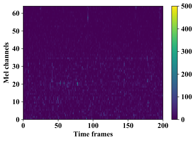
As Figure 4 shows, non-stationarity can be seen in the valve and the slider sound, where the proposed IDNN outperformed the conventional approach. For the following discussions, the performances were compared based on an example of the valve sound.
Figures 7 and 8 show the restored output for the normal and abnormal sound of the valve, respectively. As shown in Figure 7, both the AE and IDNN removed noises well and showed small errors with the normal sound. Meanwhile, in the case of the anomalous sound (see Figure 8), the error (i.e., anomaly score) of IDNN was properly large while the AE showed a smaller error than that of IDNN. As Figure 8 shows, the spectrogram reconstructed by IDNN was similar to that of the normal valve, indicating that IDNN was accurately trained for non-stationarity. In contrast, the error of PDNN was large without regarding normality, indicating that predicting the edge frame is more difficult than interpolating the center frame. Additionally, as shown in Figure 5, IDNN and PDNN showed similar performance with the slider sound, while IDNN performed much better than PDNN with the valve sound. In terms of the characteristics of the sound, the sound changes of the valve were shorter than the slider (see Figure 4), indicating that the sound change in a shorter duration made predicting the edge frame more difficult, and IDNN can be more robust in such a situation.
5 Conclusion
We proposed an approach to anomalous sound detection that employs an interpolation error of AE/VAE as an anomaly score that avoids the difficulty of predicting the edge frame. Experimental results showed that our approach outperformed conventional approaches for the non-stationary sound in particular. In the study, the number of input frames and the output were set to four and one, respectively. Further studies are needed in order to assess how those parameters can affect the detection rate.
References
- [1] Atsushi Yamashita, Takahiro Hara, and Toru Kaneko, “Inspection of visible and invisible features of objects with image and sound signal processing,” in 2006 IEEE/RSJ International Conference on Intelligent Robots and Systems. IEEE, 2006, pp. 3837–3842.
- [2] Yuma Koizumi, Shoichiro Saito, Hisashi Uematsu, and Noboru Harada, “Optimizing acoustic feature extractor for anomalous sound detection based on neyman-pearson lemma,” in 2017 25th European Signal Processing Conference (EUSIPCO). IEEE, 2017, pp. 698–702.
- [3] Varun Chandola, Arindam Banerjee, and Vipin Kumar, “Anomaly detection: A survey,” ACM computing surveys (CSUR), vol. 41, no. 3, pp. 15, 2009.
- [4] Erik Marchi, Fabio Vesperini, Florian Eyben, Stefano Squartini, and Björn Schuller, “A novel approach for automatic acoustic novelty detection using a denoising autoencoder with bidirectional lstm neural networks,” in 2015 IEEE International Conference on Acoustics, Speech and Signal Processing (ICASSP). IEEE, 2015, pp. 1996–2000.
- [5] Yohei Kawaguchi and Takashi Endo, “How can we detect anomalies from subsampled audio signals?,” in 2017 IEEE 27th International Workshop on Machine Learning for Signal Processing (MLSP). IEEE, 2017, pp. 1–6.
- [6] Takaaki Tagawa, Yukihiro Tadokoro, and Takehisa Yairi, “Structured denoising autoencoder for fault detection and analysis,” in Asian Conference on Machine Learning, 2015, pp. 96–111.
- [7] Erik Marchi, Fabio Vesperini, Felix Weninger, Florian Eyben, Stefano Squartini, and Björn Schuller, “Non-linear prediction with ’lstm’ recurrent neural networks for acoustic novelty detection,” in 2015 International Joint Conference on Neural Networks (IJCNN). IEEE, 2015, pp. 1–7.
- [8] Pascal Vincent, Hugo Larochelle, Isabelle Lajoie, Yoshua Bengio, and Pierre-Antoine Manzagol, “Stacked denoising autoencoders: Learning useful representations in a deep network with a local denoising criterion,” Journal of Machine Learning Research, vol. 11, no. Dec, pp. 3371–3408, 2010.
- [9] Diederik P Kingma and Max Welling, “Auto-encoding variational bayes,” in Proceedings of the International Conference on Learning Representations (ICLR), 2014.
- [10] Jinwon An and Sungzoon Cho, “Variational autoencoder based anomaly detection using reconstruction probability,” Special Lecture on IE, vol. 2, no. 1, 2015.
- [11] Yuta Kawachi, Yuma Koizumi, and Noboru Harada, “Complementary set variational autoencoder for supervised anomaly detection,” in 2018 IEEE International Conference on Acoustics, Speech and Signal Processing (ICASSP). IEEE, 2018, pp. 2366–2370.
- [12] Harsh Purohit, Ryo Tanabe, Kenji Ichige, Takashi Endo, Yuki Nikaido, Kaori Suefusa, and Yohei Kawaguchi, “MIMII dataset: Sound dataset for malfunctioning industrial machine investigation and inspection,” arXiv preprint arXiv:1909.09347, 2019.
- [13] Kevin Jarrett, Koray Kavukcuoglu, Marc’Aurelio Ranzato, and Yann LeCun, “What is the best multi-stage architecture for object recognition?,” in 2009 IEEE 12th international conference on computer vision. IEEE, 2009, pp. 2146–2153.
- [14] Diederik P Kingma and Jimmy Ba, “Adam: A method for stochastic optimization,” in Proceedings of the International Conference on Learning Representations (ICLR), 2015.