跳到论文正文
W Papers独立论文阅读器 arXiv:2005.09196 论文正文 计算阅读时间 · 0%
引用这篇论文根据当前论文元数据生成,正式投稿前建议核对。


License: arXiv.org perpetual non-exclusive license
arXiv:2005.09196v3 [math.DG] 06 May 2022

A new uniform lower bound on Weil-Petersson distance

Yunhui Wu Address: Tsinghua University, Haidian District, Beijing 100084, China Email address: yunhui_wu@mail.tsinghua.edu.cn
Date: August 11, 2026
Abstract.

In this paper we study the injectivity radius based at a fixed point along Weil-Petersson geodesics. We show that the square root of the injectivity radius based at a fixed point is 0.38840.3884-Lipschitz on Teichmüller space endowed with the Weil-Petersson metric. As an application we reprove that the square root of the systole function is uniformly Lipschitz on Teichmüller space endowed with the Weil-Petersson metric, where the Lipschitz constant can be chosen to be 0.54920.5492. Applications to asymptotic geometry of moduli space of Riemann surfaces for large genus will also be discussed.

Key words and phrases: 
Uniform bound, Weil-Petersson distance, injectivity radius
1991 Mathematics Subject Classification
30F60, 53C21, 32G15

1. Introduction

Let SgS_{g} be a closed surface of genus gg (g⩾2)(g\geqslant 2), and 𝒯g\mathcal{T}_{g} be the Teichmüller space of SgS_{g}. Let Teich⁡(Sg)\Teich(S_{g}) be the space 𝒯g\mathcal{T}_{g} endowed with the Weil-Petersson metric. The mapping class group Mod​(Sg)\mbox{\rm Mod}(S_{g}) acts on Teich⁡(Sg)\Teich(S_{g}) by isometries. The moduli space ℳg\mathcal{M}_{g} of SgS_{g} endowed with the Weil-Petersson metric, is realized as the quotient Teich⁡(Sg)/Mod​(Sg)\Teich(S_{g})/\mbox{\rm Mod}(S_{g}). Let ℳ−1\mathcal{M}_{-1} be the space of complete Riemannian metrics on SgS_{g} of constant Gauss curvature −1-1. It is known that 𝒯g=ℳ−1/Diff0⁡(Sg)\mathcal{T}_{g}=\mathcal{M}_{-1}/\Diff_{0}(S_{g}) where Diff0⁡(Sg)\Diff_{0}(S_{g}) is the group of diffeomorphisms of SgS_{g} isotopic to the identity. Let p∈Sgp\in S_{g} be fixed and X~∈ℳ−1\widetilde{X}\in\mathcal{M}_{-1} be a hyperbolic metric on SgS_{g}. The injectivity radius injX~⁡(p)\inj_{\widetilde{X}}(p) of X~\widetilde{X} at pp is half of the length of a shortest nontrivial geodesic loop based at pp. The geodesic loop based at pp realizing injX~⁡(p)\inj_{\widetilde{X}}(p) may not be unique. It is known that injX~⁡(p)\inj_{\widetilde{X}}(p) is bounded from above by a positive constant only depending on gg. Let

π:ℳ−1→𝒯g\pi:\mathcal{M}_{-1}\to\mathcal{T}_{g}

be the natural projection. In order to transfer the quantity inj(⋅)⁡(p)\inj_{(\cdot)}(p) onto Weil-Petersson geodesics in 𝒯g\mathcal{T}_{g}, we make the following definition. First we recall in [RT18a, RT18b] that for a smooth path c⁡(t)⊂ℳ−1c(t)\subset\mathcal{M}_{-1}, we say c⁡(t)c(t) is a horizontal curve if for each tt, there exists a holomorphic quadratic differential Ψ⁡(t)\Psi(t) of c⁡(t)c(t) such that the variation of hyperbolic metrics satisfies ∂c⁡(t)∂t=Re⁡Ψ⁡(t)\frac{\partial c(t)}{\partial t}=\re{\Psi(t)}. A smooth path in 𝒯g\mathcal{T}_{g} can always be lifted onto a horizontal curve in ℳ−1\mathcal{M}_{-1}. Throughout this paper we always assume that parameters are proportional to arc-length parameters for both geodesics in hyperbolic surfaces and smooth Weil-Petersson paths in Teichmüller space of Riemann surfaces. It is not well-defined for inj(⋅)⁡(p)\inj_{(\cdot)}(p) on 𝒯g\mathcal{T}_{g} because point pp is clearly not invariant by diffeomorphisms of SgS_{g}. To fix this problem, we first pick the Weil-Petersson geodesic joining XX and YY, and lift this Weil-Petersson geodesic onto a horizontal curve c:[0,1]→ℳ−1c:[0,1]\to\mathcal{M}_{-1}. Then we consider the injectivity radius function injc⁡(t)⁡(p)\inj_{c(t)}(p) along c⁡([0,1])c([0,1]) which is well-defined. Now we define

Definition.

Fix a point p∈Sgp\in S_{g} (g⩾2)(g\geqslant 2). For any X,Y∈𝒯gX,Y\in\mathcal{T}_{g}, we define

|injX⁡(p)−injY⁡(p)|:=supc|injc⁡(0)⁡(p)−injc⁡(1)⁡(p)|\left|\sqrt{\inj_{X}(p)}-\sqrt{\inj_{Y}(p)}\right|:=\sup_{c}\left|\sqrt{\inj_{c(0)}(p)}-\sqrt{\inj_{c(1)}(p)}\right|

where c:[0,1]→ℳ−1c:[0,1]\to\mathcal{M}_{-1} runs over all smooth horizontal curves with π⁡(c⁡(0))=X\pi(c(0))=X, π⁡(c⁡(1))=Y\pi(c(1))=Y and π⁡(c⁡([0,1]))⊂𝒯g\pi(c([0,1]))\subset\mathcal{T}_{g} is the Weil-Petersson geodesic joining XX and YY.

The definition above actually does not depend on the choice of pp. One may see the following remark for an equivalent definition.

Remark.

It is known that any two horizontal lifts in ℳ−1\mathcal{M}_{-1} of a smooth curve in 𝒯g\mathcal{T}_{g} differ by an element in Diff0⁡(Sg)\Diff_{0}(S_{g}) (see e.g. [Tro92, Chapter 22]), and the group Diff0⁡(Sg)\Diff_{0}(S_{g}) acts transitively on SgS_{g}. So the definition above is equivalent to

|injX⁡(p)−injY⁡(p)|:=supq∈Sg|injc′​(0)⁡(q)−injc′​(1)⁡(q)|\left|\sqrt{\inj_{X}(p)}-\sqrt{\inj_{Y}(p)}\right|:=\sup\limits_{q\in S_{g}}\left|\sqrt{\inj_{c^{\prime}(0)}(q)}-\sqrt{\inj_{c^{\prime}(1)}(q)}\right|

where c′:[0,1]→ℳ−1c^{\prime}:[0,1]\to\mathcal{M}_{-1} is a horizontal lift of the Weil-Petersson geodesic joining XX and YY.

In this paper, we show that

Theorem 1.1.

Fix a point p∈Sgp\in S_{g} (g⩾2)(g\geqslant 2). Then for any X,Y∈𝒯gX,Y\in\mathcal{T}_{g},

|injX⁡(p)−injY⁡(p)|⩽0.3884​distw​p⁡(X,Y)\left|\sqrt{\inj_{X}(p)}-\sqrt{\inj_{Y}(p)}\right|\leqslant 0.3884\dist_{wp}(X,Y)

where distw​p\dist_{wp} is the Weil-Petersson distance.

Remark.

Rupflin and Topping in [RT18a, Section 2] showed that

|injX⁡(p)−injY⁡(p)|⩽c⁡(g)​distw​p⁡(X,Y)\left|\sqrt{\inj_{X}(p)}-\sqrt{\inj_{Y}(p)}\right|\leqslant c(g)\dist_{wp}(X,Y)

where c⁡(g)>0c(g)>0 is a constant depending on gg. Our approach is similar to that of Rupflin and Topping, but using a detailed analysis of injectivity radius along shortest geodesic loops and a recent uniform bound for harmonic Beltrami differentials on thin parts [BW21], we are able to obtain the above uniform bound independent of gg. The Lipschitz constant 0.38840.3884 above is not optimal. More refined arguments in this proof can improve this uniform constant. In general, it is difficult to measure the Weil-Petersson distance on 𝒯g\mathcal{T}_{g}. One may see [Bro03, BBB19, BB22, CP12, KM18, RT18a, Sch13, Sch20, Wol08, Wu19] for related bounds on Weil-Petersson distances.

Recall that the systole ℓs​y​s​(X)\ell_{sys}(X) of X∈𝒯gX\in\mathcal{T}_{g} is the length of a shortest nontrivial closed geodesic in XX. Which is also the same as 2​minp∈X~​injX~⁡(p)2\min_{p\in\widetilde{X}}\inj_{\widetilde{X}}(p) where X~∈ℳ−1\widetilde{X}\in\mathcal{M}_{-1} is a hyperbolic metric on SgS_{g} with π⁡(X~)=X∈𝒯g\pi(\widetilde{X})=X\in\mathcal{T}_{g}. As a direct application of Theorem 1.1, we prove

Corollary 1.2.

For any X,Y∈𝒯gX,Y\in\mathcal{T}_{g} (g⩾2)(g\geqslant 2),

|ℓs​y​s​(X)−ℓs​y​s​(Y)|⩽0.5492​distw​p⁡(X,Y).\left|\sqrt{\ell_{sys}(X)}-\sqrt{\ell_{sys}(Y)}\right|\leqslant 0.5492\dist_{wp}(X,Y).
Proof.

Without loss of generality, one may assume that

ℓs​y​s​(X)⩾ℓs​y​s​(Y).\ell_{sys}(X)\geqslant\ell_{sys}(Y).

Let c:[0,1]→ℳ−1c:[0,1]\to\mathcal{M}_{-1} be a horizontal curve with π⁡(c⁡(0))=X\pi(c(0))=X, π⁡(c⁡(1))=Y\pi(c(1))=Y and π⁡(c⁡([0,1]))⊂𝒯g\pi(c([0,1]))\subset\mathcal{T}_{g} is the Weil-Petersson geodesic joining XX and YY. Let α⊂c⁡(1)\alpha\subset c(1) be a shortest closed geodesic. So for any p∈αp\in\alpha, we have

2​injc⁡(1)⁡(p)=ℓs​y​s​(Y)​a​n​d2​injc⁡(0)⁡(p)⩾ℓs​y​s​(X).2\inj_{c(1)}(p)=\ell_{sys}(Y)\quad\emph{and}\quad 2\inj_{c(0)}(p)\geqslant\ell_{sys}(X).

Then by Theorem 1.1 we get

ℓs​y​s​(X)−ℓs​y​s​(Y)⩽2​injc⁡(0)​(p)−2​injc⁡(1)​(p)⩽0.5492​distw​p⁡(X,Y)\sqrt{\ell_{sys}(X)}-\sqrt{\ell_{sys}(Y)}\leqslant\sqrt{2\inj_{c(0)}(p)}-\sqrt{2\inj_{c(1)}(p)}\leqslant 0.5492\dist_{wp}(X,Y)

as desired. ∎

Remark.
  1. (1)

    It was shown in [Wu19] that

    |ℓs​y​s​(X)−ℓs​y​s​(Y)|⩽K​distw​p⁡(X,Y)\left|\sqrt{\ell_{sys}(X)}-\sqrt{\ell_{sys}(Y)}\right|\leqslant K\dist_{wp}(X,Y)

    where K>0K>0 is a uniform (implicit) constant independent of gg.

  2. (2)

    Very recently, Bridgeman-Bromberg in [BB22] show that the uniform constant KK above can be chosen to be 12\frac{1}{2} by a completely different method.

Both the proofs in [Wu19] and [BB22] rely on certain uniform bound for the Weil-Petersson norm ‖∇(ℓα​(X))‖w​p||\nabla(\ell_{\alpha}(X))||_{wp} of the Weil-Petersson gradient ∇(ℓα​(X))\nabla(\ell_{\alpha}(X)) of the geodesic length function ℓα​(⋅)\ell_{\alpha}(\cdot) on Teichmüller space, where α⊂X\alpha\subset X is a systolic curve (one may also see [Wu20] for a different proof). In this paper, our proof is totally different without any estimation on ‖∇(ℓα​(X))‖w​p||\nabla(\ell_{\alpha}(X))||_{wp}. Moreover, we are able to obtain the explicit Lipschitz constant above to be 0.54920.5492, which can be improved by more careful arguments for the proof of Theorem 1.1.

The Weil-Petersson completion of the moduli space ℳg\mathcal{M}_{g} is compact which is homeomorphic to the Deligne-Mumford compactification of the moduli space of Riemann surfaces. In particular, the moduli space ℳg\mathcal{M}_{g} has finite Weil-Petersson diameter and inradius. Cavendish-Parlier [CP12] showed that for large genus the ratio diam⁡(ℳg)g\frac{\diam(\mathcal{M}_{g})}{\sqrt{g}} is bounded below by a uniform positive constant and above by a uniform constant multiple of ln⁡(g)\ln(g). It is an open problem that whether the Weil-Petersson diameter diam⁡(ℳg)\diam(\mathcal{M}_{g}) of ℳg\mathcal{M}_{g} is uniformly comparable to g​ln⁡(g)\sqrt{g}\ln(g). Recall that the Weil-Petersson inradius InRad⁡(ℳg)\Inrad(\mathcal{M}_{g}) of ℳg\mathcal{M}_{g} is defined as

InRad⁡(ℳg):=maxX∈ℳg⁡distw​p⁡(X,∂ℳg)\Inrad(\mathcal{M}_{g}):=\max_{X\in\mathcal{M}_{g}}\dist_{wp}(X,\partial\mathcal{M}_{g})

where ∂ℳg\partial\mathcal{M}_{g} is the boundary of ℳg\mathcal{M}_{g} consisting of nodal surfaces. It was shown in [Wu19] that as g→∞g\to\infty, the Weil-Petersson inradius InRad⁡(ℳg)\Inrad(\mathcal{M}_{g}) is uniformly comparable to ln⁡(g)\sqrt{\ln(g)}. More precisely, there exists a uniform constant K′>0K^{\prime}>0 independent of gg such that

K′⩽InRad⁡(ℳg)ln⁡(g)⩽4​πK^{\prime}\leqslant\frac{\Inrad(\mathcal{M}_{g})}{\sqrt{\ln(g)}}\leqslant\sqrt{4\pi}

where the uniform (implicit) constant K′K^{\prime} depends on the work of Buser-Sarnak [BS94]. The following question is natural and interesting.

Question 1.

Does limg→∞InRad⁡(ℳg)ln⁡(g)\lim\limits_{g\to\infty}\frac{\Inrad(\mathcal{M}_{g})}{\sqrt{\ln(g)}} exist? If exists, what is its value?

Set

sys⁡(g)=maxX∈ℳg⁡ℓs​y​s​(X).\sys(g)=\max_{X\in\mathcal{M}_{g}}\ell_{sys}(X).

It is known that

ℓs​y​s​(X)⩽2​ln⁡(4​g−2)\ell_{sys}(X)\leqslant 2\ln(4g-2)

for all X∈ℳgX\in\mathcal{M}_{g}. Buser and Sarnak in [BS94] showed that

sys⁡(g)⩾U​ln⁡(g)\sys(g)\geqslant U\ln(g)

for some uniform constant U>0U>0. Moreover, they also showed that there exists a sequence {gk}k⩾1\{g_{k}\}_{k\geqslant 1} of positive integers tending to infinity such that for each gkg_{k}, there exists a closed hyperbolic surface 𝒳gk\mathcal{X}_{g_{k}} of genus gkg_{k} with

ℓs​y​s​(𝒳gk)⩾4​ln⁡(gk)3−U′\ell_{sys}(\mathcal{X}_{g_{k}})\geqslant\frac{4\ln(g_{k})}{3}-U^{\prime}

where U′>0U^{\prime}>0 is a uniform constant independent of gg. Thus, the quantity sys⁡(g)\sys(g) is uniformly comparable to ln⁡(g)\ln(g) as g→∞g\to\infty. Moreover

43⩽lim supg→∞sys⁡(g)ln⁡(g)⩽2.\frac{4}{3}\leqslant\limsup_{g\to\infty}\frac{\sys(g)}{\ln(g)}\leqslant 2.

By applying the proof of Theorem 1.1 it is not hard to see that

2.0472⩽lim infg→∞InRad⁡(ℳg)sys⁡(g)⩽2.50662.0472\leqslant\liminf_{g\to\infty}\frac{\Inrad(\mathcal{M}_{g})}{\sqrt{\sys(g)}}\leqslant 2.5066

and

2.3696⩽lim supg→∞InRad⁡(ℳg)ln⁡(g)⩽3.5449.2.3696\leqslant\limsup_{g\to\infty}\frac{\Inrad(\mathcal{M}_{g})}{\sqrt{\ln(g)}}\leqslant 3.5449.

In this paper we show that

Theorem 1.3.

The following limit holds:

limg→∞InRad⁡(ℳg)sys⁡(g)=2​π∼2.5066.\lim_{g\to\infty}\frac{\Inrad(\mathcal{M}_{g})}{\sqrt{\sys(g)}}=\sqrt{2\pi}\sim 2.5066.
Remark.
  1. (1)

    Theorem 1.3 was firstly obtained in [BB22] by Bridgeman and Bromberg. We are grateful to M. Bridgeman for kindly sharing their latest version of [BB22].

  2. (2)

    The proof of [BB22] relies on bounds of ‖∇(ℓα​(X))‖w​p||\nabla(\ell_{\alpha}(X))||_{wp} in terms of functions on collars. Our proof is a slightly refined argument of the proof of [Wu19, Theorem 1.1] where we bound ‖∇(ℓα​(X))‖w​p||\nabla(\ell_{\alpha}(X))||_{wp} in terms of functions on hyperbolic disks. In both cases, α\alpha is a systolic curve of XX.

Theorem 1.3 reduces Question 1 to study the following one which has no metric involved on ℳg\mathcal{M}_{g}.

Question 2.

Does limg→∞sys⁡(g)ln⁡(g)\lim\limits_{g\to\infty}\frac{\sys(g)}{\ln(g)} exist? If exists, what is its value?

Recall that for any hyperbolic surface X∈ℳgX\in\mathcal{M}_{g}, the Bers’ constant ℬg​(X)\mathcal{B}_{g}(X) at XX is the smallest positive number such that there exist (3​g−3)(3g-3) disjoint simple closed geodesics {γi}i=13​g−3\{\gamma_{i}\}_{i=1}^{3g-3} on XX with

max1⩽i⩽(3​g−3)⁡ℓγi​(X)⩽ℬg​(X).\max_{1\leqslant i\leqslant(3g-3)}\ell_{\gamma_{i}}(X)\leqslant\mathcal{B}_{g}(X).

It is known [Bus10, Chapter 5] that

6​g−2⩽supX∈ℳgℬg​(X)⩽26​(g−1).\sqrt{6g}-2\leqslant\sup_{X\in\mathcal{M}_{g}}\mathcal{B}_{g}(X)\leqslant 26(g-1).

Buser [Bus10] conjectures that supX∈ℳgℬg​(X)\sup_{X\in\mathcal{M}_{g}}\mathcal{B}_{g}(X) is uniformly comparable to g\sqrt{g}. Fix any L>0L>0, we set the subset ℳ​𝒞(⩽L)⊆ℳg\MC(\leqslant L)\subseteq\mathcal{M}_{g} as

ℳ​𝒞(⩽L):={X∈ℳg;ℬg​(X)⩽L}.\mathcal{MC}(\leqslant L):=\left\{X\in\mathcal{M}_{g};\ \mathcal{B}_{g}(X)\leqslant L\right\}.

So ℳ​𝒞(⩽supX∈ℳgℬg​(X))=ℳg\mathcal{MC}\left(\leqslant\sup_{X\in\mathcal{M}_{g}}\mathcal{B}_{g}(X)\right)=\mathcal{M}_{g}. Let Lg=ϵ​ln⁡(g)L_{g}=\epsilon\ln(g) for large gg and small enough ϵ>0\epsilon>0. By applying [Mir13] and Theorem 1.1, we show that for large enough gg, the 1.0511​ln⁡(g)1.0511\sqrt{\ln(g)}-neighbourhood of ℳ​𝒞(⩽Lg)\mathcal{MC}(\leqslant L_{g}) can be arbitrarily small in ℳg\mathcal{M}_{g} in the following sense.

Theorem 1.4.

For any small enough ϵ>0\epsilon>0 and if Lg=ϵ​ln⁡(g)L_{g}=\epsilon\ln(g), then

limg→∞Vol_{WP}⁡({X∈ℳg;distw​p⁡(X,ℳ​𝒞(⩽Lg))>1.0511​ln⁡(g)})Vol_{WP}⁡(ℳg)=1\lim_{g\to\infty}\frac{\Vol\left(\left\{X\in\mathcal{M}_{g};\ \dist_{wp}\left(X,\mathcal{MC}(\leqslant L_{g})\right)>1.0511\sqrt{\ln(g)}\right\}\right)}{\Vol(\mathcal{M}_{g})}=1

where Vol_{WP}⁡(⋅)\Vol(\cdot) is the Weil-Petersson volume.

Plan of the paper. Section 2 provides some necessary background and the basic properties on two-dimensional hyperbolic geometry and Teichmüller theory. In Section 3 we prove two bounds for the injectivity radius along a shortest geodesic loop based at a fixed point. A technical inequality is provided in Section 4 which is crucial in the proof of Theorem 1.1. In Section 5 we finish the proof of Theorem 1.1. Theorem 1.3 is shown in Section 6. And we prove Theorem 1.4 in Section 7.

Acknowledgements. The author would like to thank Martin Bridgeman, Ran Ji and Scott Wolpert for helpful conversations on this paper, and thank to Melanie Rupflin, Peter Topping and Shing-Tung Yau for their interests. He especially would like to thank Peter Topping for useful discussions on the Definition on Page 22. He is also very grateful to anonymous referees for their helpful comments. This work is supported by the NSFC grant No. 1217126312171263 and a grant from Tsinghua University.

2. Preliminaries

In this section we will set up the notations and provide some necessary background on two-dimensional hyperbolic geometry and Teichmüller theory of Riemann surfaces.

2.1. Injectivity radius at a point

Let XX be a closed hyperbolic surface. Since the curvature of XX is −1-1, the conjugate radius at any point of XX is infinity. Thus for any point p∈Xp\in X, the injectivity radius injX⁡(p)\inj_{X}(p) of XX at pp is half of the length of a shortest nontrivial geodesic loop based at pp. Let

σ:[0,2​injX⁡(p)]→X\sigma:[0,2\inj_{X}(p)]\to X

be such a shortest geodesic loop with σ⁡(0)=σ⁡(2​injX⁡(p))=p\sigma(0)=\sigma(2\inj_{X}(p))=p of arc-length parameter. Then

  1. (1)

    the restriction σ:[0,injX⁡(p)]→X\sigma:[0,\inj_{X}(p)]\to X is a minimizing geodesic;

  2. (2)

    the restriction σ:[injX⁡(p),2​injX⁡(p)]→X\sigma:[\inj_{X}(p),2\inj_{X}(p)]\to X is also a minimizing geodesic.

For any r>0r>0, we let

B⁡(p,r):={q∈X;dist⁡(q,p)<r}B(p;r):=\left\{q\in X;\ \dist(q,p)<r\right\}

be the open geodesic ball centered at pp of radius rr. The open ball B⁡(p,injX⁡(p))B(p;\inj_{X}(p)) is an embedded hyperbolic open disk of radius injX⁡(p)\inj_{X}(p). By the Gauss-Bonnet formula we know that Area⁡(X)=4​π​(g−1)\Area(X)=4\pi(g-1). Thus,

Area⁡(B⁡(p,injX⁡(p)))=2​π​(cosh⁡(injX⁡(p))−1)⩽4​π​(g−1)\Area(B(p;\inj_{X}(p)))=2\pi\left(\cosh(\inj_{X}(p))-1\right)\leqslant 4\pi(g-1)

which implies that for any p∈Xp\in X,

(2.1) injX⁡(p)⩽ln⁡(4​g−2).\displaystyle\inj_{X}(p)\leqslant\ln(4g-2).

We remark here that for all g⩾2g\geqslant 2, Buser and Sarnak in [BS94] constructed a closed surface 𝒳g\mathcal{X}_{g} of genus gg such that

infp∈𝒳ginj𝒳g⁡(p)⩾U​ln⁡(g)\inf_{p\in\mathcal{X}_{g}}\inj_{\mathcal{X}_{g}}(p)\geqslant U\ln(g)

for some uniform constant U>0U>0 independent of gg.

2.2. Teichmüller space and Weil-Petersson metric.

We denote by SgS_{g} an oriented closed surface of genus gg (g⩾2)(g\geqslant 2). The Uniformization Theorem implies that the surface SgS_{g} admits hyperbolic metrics of constant curvature −1-1. We let 𝒯g\mathcal{T}_{g} be the Teichmüller space of surfaces of genus gg, which we consider as the equivalence classes under the action of the group Diff0⁡(Sg)\Diff_{0}(S_{g}) of diffeomorphisms isotopic to the identity of the space of hyperbolic surfaces X=(Sg,σ⁡(z)​|d​z|2)X=(S_{g},\sigma(z)|dz|^{2}). The tangent space TX​𝒯gT_{X}\mathcal{T}_{g} at a point X=(Sg,σ⁡(z)​|d​z|2)X=(S_{g},\sigma(z)|dz|^{2}) is identified with the space of harmonic Beltrami differentials on XX, i.e., forms on XX expressible as μ=ψ¯/σ\mu=\overline{\psi}/\sigma where ψ∈Q⁡(X)\psi\in Q(X) is a holomorphic quadratic differential on XX. The pointwise norm |μ⁡(⋅)|:X→ℝ⩾0|\mu(\cdot)|:X\to\mathbb{R}^{\geqslant 0} gives a continuous nonnegative function on XX. Let z=x+i​yz=x+iy and dArea=σ⁡(z)​d​x​d​y\dArea=\sigma(z)dxdy be the volume form. The Weil-Petersson metric is the Hermitian metric on 𝒯g\mathcal{T}_{g} arising from the the Petersson scalar product

⟨φ,ψ⟩=∫Xφ⋅ψ¯σ2​dArea\left<\varphi,\psi\right>=\int_{X}\frac{\varphi\cdot\overline{\psi}}{\sigma^{2}}\dArea

via duality. We will concern ourselves primarily with its Riemannian part gW​Pg_{WP}. Throughout this paper we denote by Teich⁡(Sg)\Teich(S_{g}) the Teichmüller space endowed with the Weil-Petersson metric. By definition it is easy to see that the mapping class group Mod​(Sg)\mbox{\rm Mod}(S_{g}) acts on Teich⁡(Sg)\Teich(S_{g}) as isometries. Thus, the Weil-Petersson metric descends to a metric, also called the Weil-Petersson metric, on the moduli space of Riemann surfaces ℳg\mathcal{M}_{g} which is defined as 𝒯g/Mod​(Sg)\mathcal{T}_{g}/\mbox{\rm Mod}(S_{g}). Throughout this paper we also denote by ℳg\mathcal{M}_{g} the moduli space endowed with the Weil-Petersson metric. One may refer to [IT92, Wol10] for more details on Weil-Petersson geometry.

2.3. Uniform bounds on harmonic Beltrami differentials

In this subsection we recall two uniform bounds on the pointwise norm of any harmonic Beltrami differential in terms of the injectivity radius at a point. We first refer to a function C⁡(r)C(r) introduced by Teo in [Teo09] which is given by

(2.2) C⁡(r)=(4​π3​(1−(4​er(1+er)2)3))−12.\displaystyle C(r)=\left(\frac{4\pi}{3}\left(1-\left(\frac{4e^{r}}{(1+e^{r})^{2}}\right)^{3}\right)\right)^{-\frac{1}{2}}.

It follows that C⁡(r)C(r) is decreasing with respect to rr and as rr tends to zero we have

C⁡(r)=1π​r+O⁡(1).C(r)=\frac{1}{\sqrt{\pi}r}+O(1).

Furthermore C⁡(r)C(r) tends to 34​π\sqrt{\frac{3}{4\pi}} as rr tends to infinity. The following property follows by a Taylor expansion of μ\mu on a hyperbolic disk of radius r>0r>0.

Proposition 2.1 (Teo, [Teo09, Prop 3.1] or [WW18, Prop 2.10]).

Let XX be a closed hyperbolic surface and μ\mu be a harmonic Beltrami differential on XX. Then for any p∈Xp\in X,

|μ⁡(p)|2⩽(C⁡(injX⁡(p)))2​∫B⁡(p,r)|μ⁡(z)|2​dArea⁡(z),∀ 0<r⩽injX⁡(p)|\mu(p)|^{2}\leqslant\left(C(\inj_{X}(p))\right)^{2}\int_{B(p;r)}{|\mu(z)|^{2}\dArea(z)},\ \forall\ 0<r\leqslant\inj_{X}(p)

where the constant C⁡(⋅)C(\cdot) is given by (2.2).

Proposition 2.1 is useful when the injectivity radius at a point is uniformly bounded from below, especially as the injectivity radius goes to infinity. For the case that the injectivity radius at a point is small, we will use the following recent result, which follows by a detailed analysis on the Fourier expansion of μ\mu on a collar of a short closed geodesic. More precisely,

Proposition 2.2 (Bridgeman-Wu, [BW21, Prop 1.1]).

Let XX be a closed hyperbolic surface and μ\mu be a harmonic Beltrami differential on XX. Then for any p∈Xp\in X with injX⁡(p)⩽arcsinh⁡(1)\inj_{X}(p)\leqslant\arcsinh(1),

|μ⁡(p)|2⩽∫X|μ⁡(z)|2​dArea⁡(z)injX⁡(p).|\mu(p)|^{2}\leqslant\frac{\int_{X}|\mu(z)|^{2}\dArea(z)}{\inj_{X}(p)}.

3. Two bounds on injectivity radius

Let XX be a closed hyperbolic surface of genus g⩾2g\geqslant 2 and γ⊂X\gamma\subset X be a non-trivial simple loop. There always exists a unique closed geodesic, still denoted by γ\gamma, representing this loop. The Collar Lemma says that it has a tubular neighborhood which is a topological cylinder with a standard hyperbolic metric. And the width of this cylinder, only depending on the length of γ\gamma, goes to infinity as the length of γ\gamma goes to 00. First we recall the following version of the Collar Lemma which will be applied.

Theorem 3.1.

[Bus10, Theorem 4.1.1] Let γ1,γ2,…,γm\gamma_{1},\gamma_{2},...,\gamma_{m} be disjoint simple closed geodesics on a closed hyperbolic Riemann surface XX of genus gg, and ℓ⁡(γi)\ell(\gamma_{i}) be the length of γi\gamma_{i}. Then m⩽3​g−3m\leqslant 3g-3 and we can define the collar of γi\gamma_{i} by

𝒞⁡(γi)={x∈Xg;dist⁡(x,γi)⩽w⁡(γi)}\mathcal{C}(\gamma_{i})=\{x\in X_{g};\ \dist(x,\gamma_{i})\leqslant w(\gamma_{i})\}

where

w⁡(γi)=arcsinh(1sinh⁡12​ℓ​(γi))w(\gamma_{i})=\mathop{\rm arcsinh}\left(\frac{1}{\sinh\frac{1}{2}\ell(\gamma_{i})}\right)

is the half width of the collar.

Then the collars are pairwise disjoint for i=1,…,mi=1,...,m. Each 𝒞⁡(γi)\mathcal{C}(\gamma_{i}) is isomorphic to a cylinder (ρ,t)∈[−w⁡(γi),w⁡(γi)]×𝕊1(\rho,t)\in[-w(\gamma_{i}),w(\gamma_{i})]\times\mathbb{S}^{1}, where 𝕊1=ℝ/ℤ\mathbb{S}^{1}=\mathbb{R}/\mathbb{Z}, with the metric

(3.1) d​s2=d​ρ2+ℓ​(γi)2​cosh2⁡ρ​d​t2.\displaystyle ds^{2}=d\rho^{2}+\ell(\gamma_{i})^{2}\cosh^{2}\rho dt^{2}.

And for a point (ρ,t)(\rho,t), the point (0,t)(0,t) is its projection on the geodesic γi\gamma_{i}, the absolute value |ρ|\lvert\rho\rvert is the distance to γi\gamma_{i}, tt is the coordinate on γi≅𝕊1\gamma_{i}\cong\mathbb{S}^{1}.

As the length ℓ⁡(γ)\ell(\gamma) of the central closed geodesic goes to 00, the width

(3.2) ew⁡(γ)∼4ℓ⁡(γ)\displaystyle e^{w(\gamma)}\sim\frac{4}{\ell(\gamma)}

which tends to infinity. In this paper, we mainly deal with the case that ℓ⁡(γ)\ell(\gamma) is small and so w⁡(γ)w(\gamma) is large.

Now we recall another version of the Collar Lemma which provides useful information on the injectivity radius at a point.

Theorem 3.2.

[Bus10, Theorem 4.1.6] Let β1,⋯,βk\beta_{1},\cdots,\beta_{k} be the set of all simple closed geodesics of length ⩽2​arcsinh⁡(1)\leqslant 2\arcsinh(1) on a closed hyperbolic Riemann surface XX of genus gg. Then k⩽3​g−3k\leqslant 3g-3, and the followings hold.

  1. (1)

    The geodesics β1,⋯,βk\beta_{1},\cdots,\beta_{k} are pairwise disjoint

  2. (2)

    injX⁡(p)>arcsinh⁡(1)\inj_{X}(p)>\arcsinh(1) for any p∈X∖(∪i=1k𝒞(βi))p\in X\setminus(\cup_{i=1}^{k}\mathcal{C}(\beta_{i})).

  3. (3)

    If p∈𝒞⁡(βi)p\in\mathcal{C}(\beta_{i}), and d⁡(p)=dist⁡(p,∂𝒞⁡(βi))d(p)=\dist(p,\partial\mathcal{C}(\beta_{i})), then

    (3.3) sinh⁡(injX⁡(p))=cosh⁡(ℓ⁡(βi)2)​cosh⁡(d⁡(p))−sinh⁡(d⁡(p)),\displaystyle\sinh(\inj_{X}(p))=\cosh\left(\frac{\ell(\beta_{i})}{2}\right)\cosh\left(d(p))-\sinh(d(p)\right),
    (3.4) sinh⁡(injX⁡(p))=sinh⁡(ℓ⁡(βi)2)​cosh⁡(dist⁡(p,βi))​​(s​e​e​[Bus10, 4.1.7])\displaystyle\quad\quad\quad\sinh(\inj_{X}(p))=\sinh\left(\frac{\ell(\beta_{i})}{2}\right)\cosh(\dist(p,\beta_{i}))\ \emph{(see\cite[cite]{[\@@bibref{}{Buser10}{}{}, 4.1.7]})}

By comparing the total area of all these standard collars 𝒞​(βi)′​s\mathcal{C}(\beta_{i})^{\prime}s and the total area 4​π​(g−1)4\pi(g-1) of XX, the set X∖(∪i=1k𝒞(βi))X\setminus(\cup_{i=1}^{k}\mathcal{C}(\beta_{i})) is always non-empty. And for any point q∈∂𝒞⁡(βi)q\in\partial\mathcal{C}(\beta_{i}), by continuity or (3.3) we know that injX⁡(q)⩾arcsinh⁡(1)\inj_{X}(q)\geqslant\arcsinh(1). Now we study the injectivity radius along shortest geodesic loops (may not smooth at base points). First we consider the case that the base point is contained in a collar with a central closed geodesic of length ⩽2​arcsinh⁡(1)\leqslant 2\arcsinh(1).

Proposition 3.3.

Let XX be a closed hyperbolic surface. For any p∈Xp\in X with injX⁡(p)⩽arcsinh⁡(1)\inj_{X}(p)\leqslant\arcsinh(1), we let σ:[0,2​injX⁡(p)]→X\sigma:[0,2\inj_{X}(p)]\to X be a shortest nontrivial geodesic loop based at pp. Then for any s∈[0,2​injX⁡(p)]s\in[0,2\inj_{X}(p)], we have

(2−1)​injX⁡(p)⩽injX⁡(σ⁡(s))⩽injX⁡(p).\left(\sqrt{2}-1\right)\inj_{X}(p)\leqslant\inj_{X}(\sigma(s))\leqslant\inj_{X}(p).
Proof.

Since injX⁡(p)⩽arcsinh⁡(1)\inj_{X}(p)\leqslant\arcsinh(1), by Theorem 3.1 and 3.2 one may assume that β\beta is the unique simple closed geodesic of length ⩽2​arcsinh⁡(1)\leqslant 2\arcsinh(1) such that p∈𝒞⁡(β)p\in\mathcal{C}(\beta). So the shortest geodesic loop

σ⁡([0,2​injX⁡(p)])⊂𝒞⁡(β)\sigma([0,2\inj_{X}(p)])\subset\mathcal{C}(\beta)

otherwise it follows by Theorem 3.2 that σ⁡([0,2​injX⁡(p)])\sigma([0,2\inj_{X}(p)]) contains a point q∉𝒞⁡(β)q\notin\mathcal{C}(\beta) with injX⁡(q)>arcsinh⁡(1)\inj_{X}(q)>\arcsinh(1) implying that ℓ⁡(σ)>2​arcsinh⁡(1)\ell(\sigma)>2\arcsinh(1) which is a contradiction.

Now we first show the right hand side inequality: up to a conjugation one may lift β\beta onto the imaginary axis i⋅ℝ+\textbf{i}\cdot\mathbb{R}^{+} in the upper half plane ℍ\mathbb{H}, and the deck transformation corresponding to β\beta is A⁡(z)=eℓ⁡(β)​zA(z)=e^{\ell(\beta)}z. By Theorem 3.1 one may let p~\widetilde{p} be a lift of pp with

distℍ⁡(p~,i⋅ℝ+)=dist⁡(p,β)⩽arcsinh⁡(1sinh⁡12​ℓ​(β)).\dist_{\mathbb{H}}(\widetilde{p},\textbf{i}\cdot\mathbb{R}^{+})=\dist(p,\beta)\leqslant\arcsinh\left(\frac{1}{\sinh\frac{1}{2}\ell(\beta)}\right).

Then the lift σ~:[0,2​injX⁡(p)]→ℍ\widetilde{\sigma}:[0,2\inj_{X}(p)]\to\mathbb{H} of σ\sigma based at p~\widetilde{p} is the geodesic joining p~\widetilde{p} and A⁡(p~)A(\widetilde{p}) in ℍ\mathbb{H}. By the convexity of distance functions on ℍ\mathbb{H} we know that for any s∈[0,2​injX⁡(p)]s\in[0,2\inj_{X}(p)],

distℍ⁡(σ~​(s),i⋅ℝ+)⩽distℍ⁡(p~,i⋅ℝ+)=distℍ⁡(A⁡(p~),i⋅ℝ+)\dist_{\mathbb{H}}(\widetilde{\sigma}(s),\textbf{i}\cdot\mathbb{R}^{+})\leqslant\dist_{\mathbb{H}}(\widetilde{p},\textbf{i}\cdot\mathbb{R}^{+})=\dist_{\mathbb{H}}(A(\widetilde{p}),\textbf{i}\cdot\mathbb{R}^{+})

which implies that

(3.5) dist⁡(σ⁡(s),β)⩽dist⁡(p,β).\displaystyle\dist(\sigma(s),\beta)\leqslant\dist(p,\beta).

Then it follows by (3.4) that

injX⁡(σ⁡(s))⩽injX⁡(p)\inj_{X}(\sigma(s))\leqslant\inj_{X}(p)

for all s∈[0,2​injX⁡(p)]s\in[0,2\inj_{X}(p)].

Next we show the other side inequality. Let s∈[0,2​injX⁡(p)]s\in[0,2\inj_{X}(p)]. Then

(3.6) dist⁡(p,σ⁡(s))⩽injX⁡(p)⩽arcsinh⁡(1).\displaystyle\dist(p,\sigma(s))\leqslant\inj_{X}(p)\leqslant\arcsinh(1).

We finish the proof by considering the following two cases.

Case (1)(1). dist⁡(p,β)>dist⁡(p,σ⁡(s))\dist(p,\beta)>\dist(p,\sigma(s)). Let π⁡(σ⁡(s))∈β\pi(\sigma(s))\in\beta with

dist⁡(σ⁡(s),π⁡(σ⁡(s)))=dist⁡(σ⁡(s),β).\dist(\sigma(s),\pi(\sigma(s)))=\dist(\sigma(s),\beta).

By the triangle inequality we have

dist⁡(σ⁡(s),β)\displaystyle\dist(\sigma(s),\beta) ⩾\displaystyle\geqslant dist⁡(π⁡(σ⁡(s)),p)−dist⁡(p,σ⁡(s))\displaystyle\dist(\pi(\sigma(s)),p)-\dist(p,\sigma(s))
⩾\displaystyle\geqslant dist⁡(p,β)−dist⁡(p,σ⁡(s))>0.\displaystyle\dist(p,\beta)-\dist(p,\sigma(s))>0.

Then it follows by (3.4) and (3.6) that

sinh⁡(injX⁡(σ⁡(s)))\displaystyle\sinh(\inj_{X}(\sigma(s))) =\displaystyle= sinh⁡(ℓ⁡(β)2)​cosh⁡(dist⁡(σ⁡(s),β))\displaystyle\sinh\left(\frac{\ell(\beta)}{2}\right)\cosh(\dist(\sigma(s),\beta))
⩾\displaystyle\geqslant sinh⁡(ℓ⁡(β)2)​cosh⁡(dist⁡(p,β)−dist⁡(p,σ⁡(s)))\displaystyle\sinh\left(\frac{\ell(\beta)}{2}\right)\cosh\left(\dist(p,\beta)-\dist(p,\sigma(s))\right)
⩾\displaystyle\geqslant (sinh⁡(ℓ⁡(β)2)​cosh⁡(dist⁡(p,β)))​e−dist⁡(p,σ⁡(s))\displaystyle\left(\sinh\left(\frac{\ell(\beta)}{2}\right)\cosh(\dist(p,\beta))\right)e^{-\dist(p,\sigma(s))}
⩾\displaystyle\geqslant sinh⁡(injX⁡(p))⋅e−arcsinh⁡(1)\displaystyle\sinh(\inj_{X}(p))\cdot e^{-\arcsinh(1)}
>\displaystyle> sinh⁡(e−arcsinh⁡(1)⋅injX⁡(p)).\displaystyle\sinh\left(e^{-\arcsinh(1)}\cdot\inj_{X}(p)\right).

Thus, we have

(3.7) injX⁡(σ⁡(s))⩾e−arcsinh⁡(1)​injX⁡(p)=(2−1)​injX⁡(p).\displaystyle\inj_{X}(\sigma(s))\geqslant e^{-\arcsinh(1)}\inj_{X}(p)=\left(\sqrt{2}-1\right)\inj_{X}(p).

Which completes the proof for this case.

Case (2)(2). dist⁡(p,β)⩽dist⁡(p,σ⁡(s))\dist(p,\beta)\leqslant\dist(p,\sigma(s)). Then by (3.6) we have

(3.8) dist⁡(p,β)⩽dist⁡(p,σ⁡(s))⩽arcsinh⁡(1).\displaystyle\dist(p,\beta)\leqslant\dist(p,\sigma(s))\leqslant\arcsinh(1).

By (3.1) of Theorem 3.1, we have that the closed curve (not a geodesic loop) based at pp with equidistance dist⁡(p,β)\dist(p,\beta) to β\beta has length ℓ⁡(β)​cosh⁡(dist⁡(p,β))\ell(\beta)\cosh(\dist(p,\beta)). Which together with (3.8) implies that

injX⁡(p)<ℓ⁡(β)2​cosh⁡(arcsinh⁡(1))=22​ℓ​(β).\inj_{X}(p)<\frac{\ell(\beta)}{2}\cosh(\arcsinh(1))=\frac{\sqrt{2}}{2}\ell(\beta).

Thus, we have

(3.9) injX⁡(σ⁡(s))⩾ℓ⁡(β)2>22​injX⁡(p).\displaystyle\inj_{X}(\sigma(s))\geqslant\frac{\ell(\beta)}{2}>\frac{\sqrt{2}}{2}\inj_{X}(p).

Then the conclusion follows by (3.7) and (3.9) because 22>(2−1)\frac{\sqrt{2}}{2}>(\sqrt{2}-1). ∎

Now we consider the case that the base point has injectivity radius larger than arcsinh⁡(1)\arcsinh(1). Let β\beta be a simple closed geodesic in XX of length

ℓ⁡(β)⩽2​arcsinh⁡(1).\ell(\beta)\leqslant 2\arcsinh(1).

The boundary ∂𝒞⁡(β)\partial\mathcal{C}(\beta) of the collar 𝒞⁡(β)\mathcal{C}(\beta) are two disjoint closed curves homotopic to β\beta. By (3.1) we know that for each component β′\beta^{\prime} of ∂𝒞⁡(β)\partial\mathcal{C}(\beta), the length ℓ⁡(β′)\ell(\beta^{\prime}) of β′\beta^{\prime} is

ℓ⁡(β′)=ℓ⁡(β)​cosh⁡(ω⁡(β))=ℓ⁡(β)⋅cosh⁡(arcsinh⁡(1sinh⁡12​ℓ​(β))).\displaystyle\quad\ell(\beta^{\prime})=\ell(\beta)\cosh(\omega(\beta))=\ell(\beta)\cdot\cosh\left(\arcsinh\left(\frac{1}{\sinh\frac{1}{2}\ell(\beta)}\right)\right).

A simple computation shows that

(3.10) ℓ⁡(β′)\displaystyle\quad\ell(\beta^{\prime}) =\displaystyle= ℓ⁡(β)sinh⁡12​ℓ​(β)⋅1+(sinh⁡12​ℓ​(β))2⩽2​2.\displaystyle\frac{\ell(\beta)}{\sinh\frac{1}{2}\ell(\beta)}\cdot\sqrt{1+\left(\sinh\frac{1}{2}\ell(\beta)\right)^{2}}\leqslant 2\sqrt{2}.

Now we are ready to state the result for the other case.

Proposition 3.4.

Let XX be a closed hyperbolic surface. For any p∈Xp\in X with injX⁡(p)>arcsinh⁡(1)\inj_{X}(p)>\arcsinh(1), we let σ:[0,2​injX⁡(p)]→X\sigma:[0,2\inj_{X}(p)]\to X be a shortest nontrivial geodesic loop based at pp. Then

mins∈[0,2​injX⁡(p)]⁡injX⁡(σ⁡(s))⩾ln⁡(e−2+e−2​2+1)∼0.2407.\min_{s\in[0,2\inj_{X}(p)]}\inj_{X}(\sigma(s))\geqslant\ln\left(e^{-\sqrt{2}}+\sqrt{e^{-2\sqrt{2}}+1}\right)\sim 0.2407.
Proof.

If the geodesic loop σ\sigma does not intersect with any standard collar with central closed geodesic of length less than 2​arcsinh⁡(1)2\arcsinh(1), it follows by Theorem 3.2 that

mins∈[0,2​injX⁡(p)]⁡injX⁡(σ⁡(s))⩾arcsinh⁡(1)>ln⁡(e−2+e−2​2+1)∼0.2407.\min_{s\in[0,2\inj_{X}(p)]}\inj_{X}(\sigma(s))\geqslant\arcsinh(1)>\ln\left(e^{-\sqrt{2}}+\sqrt{e^{-2\sqrt{2}}+1}\right)\sim 0.2407.

Now we assume that

σ∩𝒞⁡(β)≠∅\sigma\cap\mathcal{C}(\beta)\neq\emptyset

for some simple closed geodesic β\beta of length less than or equal to 2​arcsinh⁡(1)2\arcsinh(1).

Claim: ∀q∈(σ∩𝒞⁡(β))\forall q\in(\sigma\cap\mathcal{C}(\beta)), dist⁡(q,∂𝒞⁡(β))⩽2\dist(q,\partial\mathcal{C}(\beta))\leqslant\sqrt{2}.

If the claim above is true, then it follows by (3.3) in Theorem 3.2 that

sinh⁡(injX⁡(q))\displaystyle\sinh(\inj_{X}(q)) =\displaystyle= cosh⁡(ℓ⁡(β)2)​cosh⁡(dist⁡(q,∂𝒞⁡(β)))−sinh⁡(dist⁡(q,∂𝒞⁡(β)))\displaystyle\cosh\left(\frac{\ell(\beta)}{2}\right)\cosh\left(\dist(q,\partial\mathcal{C}(\beta)))-\sinh(\dist(q,\partial\mathcal{C}(\beta))\right)
⩾\displaystyle\geqslant cosh⁡(dist⁡(q,∂𝒞⁡(β)))−sinh⁡(dist⁡(q,∂𝒞⁡(β)))\displaystyle\cosh\left(\dist(q,\partial\mathcal{C}(\beta)))-\sinh(\dist(q,\partial\mathcal{C}(\beta))\right)
=\displaystyle= e−dist⁡(q,∂𝒞⁡(β))\displaystyle e^{-\dist(q,\partial\mathcal{C}(\beta))}
⩾\displaystyle\geqslant e−2\displaystyle e^{-\sqrt{2}}

which implies that

injX⁡(q)⩾ln⁡(e−2+e−2​2+1)∼0.2407.\inj_{X}(q)\geqslant\ln\left(e^{-\sqrt{2}}+\sqrt{e^{-2\sqrt{2}}+1}\right)\sim 0.2407.

Since β\beta is an arbitrary closed geodesic of length less than or equal to 2​arcsinh⁡(1)2\arcsinh(1) such that σ∩𝒞⁡(β)≠∅\sigma\cap\mathcal{C}(\beta)\neq\emptyset, by Theorem 3.2 we know that

mins∈[0,2​injX⁡(p)]⁡injX⁡(σ⁡(s))⩾min⁡{arcsinh⁡(1), 0.2407}=0.2407.\min_{s\in[0,2\inj_{X}(p)]}\inj_{X}(\sigma(s))\geqslant\min\left\{\arcsinh(1),\ 0.2407\right\}=0.2407.

Now we prove the claim.

Proof of Claim. Suppose for contradiction that

dist⁡(q,∂𝒞⁡(β))>2\dist(q,\partial\mathcal{C}(\beta))>\sqrt{2}

for some q∈(σ∩𝒞⁡(β))q\in(\sigma\cap\mathcal{C}(\beta)). We let t1>0t_{1}>0 be the first time when σ\sigma meets 𝒞⁡(β)\mathcal{C}(\beta), and t2>0t_{2}>0 be the last time when σ\sigma meets 𝒞⁡(β)\mathcal{C}(\beta). That is,

t1:=min⁡{s∈[0,2​injX⁡(p)];σ⁡(s)∈𝒞⁡(β)}t_{1}:=\min\left\{s\in[0,2\inj_{X}(p)];\ \sigma(s)\in\mathcal{C}(\beta)\right\}

and

t2:=max⁡{s∈[0,2​injX⁡(p)];σ⁡(t)∈𝒞⁡(β)}.t_{2}:=\max\left\{s\in[0,2\inj_{X}(p)];\ \sigma(t)\in\mathcal{C}(\beta)\right\}.

Since injX⁡(σ⁡(0))=injX⁡(σ⁡(2​injX⁡(p)))=injX⁡(p)>arcsinh⁡(1)\inj_{X}(\sigma(0))=\inj_{X}(\sigma(2\inj_{X}(p)))=\inj_{X}(p)>\arcsinh(1), we have that t1>0t_{1}>0 and t2<2​injX⁡(p)t_{2}<2\inj_{X}(p). Clearly we have σ⁡(t1)∪σ⁡(t2)∈∂𝒞⁡(β)\sigma(t_{1})\cup\sigma(t_{2})\in\partial\mathcal{C}(\beta). If σ⁡(t1)\sigma(t_{1}) and σ⁡(t2)\sigma(t_{2}) are on the same component of the boundary ∂𝒞⁡(β)\partial\mathcal{C}(\beta), then we have

t2−t1⩾dist⁡(σ⁡(t1),q)+dist⁡(q,σ⁡(t2))>2​2.t_{2}-t_{1}\geqslant\dist(\sigma(t_{1}),q)+\dist(q,\sigma(t_{2}))>2\sqrt{2}.

If σ⁡(t1)\sigma(t_{1}) and σ⁡(t2)\sigma(t_{2}) are on the different components of the boundary ∂𝒞⁡(β)\partial\mathcal{C}(\beta), by symmetry of the standard collar 𝒞⁡(β)\mathcal{C}(\beta) we also have

t2−t1⩾2​dist⁡(q,∂𝒞⁡(β))>2​2.t_{2}-t_{1}\geqslant 2\dist(q,\partial\mathcal{C}(\beta))>2\sqrt{2}.

So we always have

(3.11) t2−t1>2​2.\displaystyle t_{2}-t_{1}>2\sqrt{2}.

Now we finish the argument by considering the following two cases.

Case (1)(1). t1=ℓ⁡(σ⁡([0,t1]))⩽ℓ⁡(σ⁡([t2,2​injX⁡(p)]))=2​injX⁡(p)−t2t_{1}=\ell(\sigma([0,t_{1}]))\leqslant\ell(\sigma([t_{2},2\inj_{X}(p)]))=2\inj_{X}(p)-t_{2}. Let β′\beta^{\prime} be the component of the boundary ∂𝒞⁡(β)\partial\mathcal{C}(\beta) with σ⁡(t1)∈β′\sigma(t_{1})\in\beta^{\prime}, and we parametrize β′\beta^{\prime} such that β′​(0)=β′​(ℓ⁡(β′))=σ⁡(t1)\beta^{\prime}(0)=\beta^{\prime}(\ell(\beta^{\prime}))=\sigma(t_{1}). Consider the closed curve σ′\sigma^{\prime} based at pp as following.

σ′​(s):={σ⁡(s),​s∈[0,t_1];β′​(s−t1),​s∈[t_1, t_1+ℓ(β’)];σ⁡(2​t1+ℓ⁡(β′)−s),​s∈[t_1+ℓ(β’), 2t_1+ℓ(β’)].\displaystyle\sigma^{\prime}(s):=\begin{cases}\sigma(s),\quad\quad\quad\ \emph{$s\in[0,t_1]$};\\ \beta^{\prime}(s-t_{1}),\quad\emph{$s\in[t_1, t_1+\ell(\beta')]$};\\ \sigma\left(2t_{1}+\ell(\beta^{\prime})-s\right),\quad\emph{$s\in[t_1+\ell(\beta'), 2t_1+\ell(\beta')]$}.\end{cases}

The closed curve σ′\sigma^{\prime} is freely homotopic to β\beta. So σ′\sigma^{\prime} is nontrivial. By (3.10) and (3.11), the length of σ′\sigma^{\prime} satisfies

ℓ⁡(σ′)\displaystyle\ell(\sigma^{\prime}) =\displaystyle= 2​t1+ℓ⁡(β′)\displaystyle 2t_{1}+\ell(\beta^{\prime})
⩽\displaystyle\leqslant t1+(2​injX⁡(p)−t2)+2​2\displaystyle t_{1}+(2\inj_{X}(p)-t_{2})+2\sqrt{2}
<\displaystyle< 2​injX​(p)\displaystyle 2\inj_{X}(p)

which is a contradiction since σ\sigma is a shortest nontrivial geodesic loop based at pp.

Case (2)(2). t1=ℓ⁡(σ⁡([0,t1]))⩾ℓ⁡(σ⁡([t2,2​injX⁡(p)]))=2​injX⁡(p)−t2t_{1}=\ell(\sigma([0,t_{1}]))\geqslant\ell(\sigma([t_{2},2\inj_{X}(p)]))=2\inj_{X}(p)-t_{2}. Let β′′\beta^{\prime\prime} be the component of the boundary ∂𝒞⁡(β)\partial\mathcal{C}(\beta) with σ⁡(t2)∈β′′\sigma(t_{2})\in\beta^{\prime\prime}. Similarly, we consider the closed curve σ′′\sigma^{\prime\prime} based at pp which is defined as

σ′′=σ⁡([t2,2​injX⁡(p)])∪β′′∪σ⁡([t2,2​injX⁡(p)]).\sigma^{\prime\prime}=\sigma([t_{2},2\inj_{X}(p)])\cup\beta^{\prime\prime}\cup\sigma([t_{2},2\inj_{X}(p)]).

Then the closed curve σ′′\sigma^{\prime\prime} is freely homotopic to β\beta. So σ′′\sigma^{\prime\prime} is nontrivial. By (3.10) and (3.11), the length of σ′′\sigma^{\prime\prime} satisfies

ℓ⁡(σ′′)\displaystyle\ell(\sigma^{\prime\prime}) =\displaystyle= 2​(2​injX⁡(p)−t2)+ℓ⁡(β′′)\displaystyle 2(2\inj_{X}(p)-t_{2})+\ell(\beta^{\prime\prime})
⩽\displaystyle\leqslant t1+(2​injX⁡(p)−t2)+2​2\displaystyle t_{1}+(2\inj_{X}(p)-t_{2})+2\sqrt{2}
<\displaystyle< 2​injX​(p)\displaystyle 2\inj_{X}(p)

which is a contradiction since σ′′\sigma^{\prime\prime} is a nontrivial closed loop based at pp.

The proof is complete. ∎

4. One useful inequality

In this section we prove the following property which is crucial in the proof of Theorem 1.1.

Proposition 4.1.

Let XX be a hyperbolic surface. For any p∈Xp\in X we let σ:[0,2​injX⁡(p)]→X\sigma:[0,2\inj_{X}(p)]\to X be a shortest nontrivial geodesic loop based at pp. Assume that

infs∈[0,2​injX⁡(p)]injX⁡(σ⁡(s))⩾2​ε0\inf_{s\in[0,2\inj_{X}(p)]}\inj_{X}(\sigma(s))\geqslant 2\varepsilon_{0}

for some uniform constant ε0>0\varepsilon_{0}>0. Then for any function f⩾0f\geqslant 0 on XX, we have

∫02​injX​(p)(∫B⁡(σ⁡(s),ε0)f​dArea)​𝑑s⩽12​ε0​∫𝒩ε0​(σ)f​dArea.\int_{0}^{2\inj_{X}(p)}\left(\int_{B(\sigma(s);\varepsilon_{0})}f\dArea\right)ds\leqslant 12\varepsilon_{0}\int_{\mathcal{N}_{\varepsilon_{0}}(\sigma)}f\dArea.

Where B⁡(σ⁡(s),ε0)={q∈X;dist⁡(q,σ⁡(s))<ε0}B(\sigma(s);\varepsilon_{0})=\{q\in X;\ \dist(q,\sigma(s))<\varepsilon_{0}\} and 𝒩ε0​(σ)\mathcal{N}_{\varepsilon_{0}}(\sigma) is the ε0\varepsilon_{0}-neighbourhood of σ\sigma, i.e.,

𝒩ε0​(σ)={z∈X;dist⁡(x,σ⁡([0,2​injX⁡(p)]))<ε0}\mathcal{N}_{\varepsilon_{0}}(\sigma)=\{z\in X;\ \dist\left(x,\sigma([0,2\inj_{X}(p)])\right)<\varepsilon_{0}\}

We split the proof into several parts.

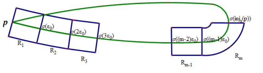
First since σ:[0,2​injX⁡(p)]→X\sigma:[0,2\inj_{X}(p)]\to X is a shortest nontrivial geodesic loop based at pp, it is known that both the two restrictions σ:[0,injX⁡(p)]→X\sigma:[0,\inj_{X}(p)]\to X and σ:[injX⁡(p),2​injX⁡(p)]→X\sigma:[\inj_{X}(p),2\inj_{X}(p)]\to X are minimizing geodesics. For any s∈(0,2​injX⁡(p))s\in(0,2\inj_{X}(p)), we let n→​(s)\vec{n}(s) be an unit normal vector of σ\sigma at σ⁡(s)\sigma(s). Consider the foliation {expσ⁡(s)⁡(t⋅n→​(s))}t∈(−ε0,ε0),t∈(0,2​injX⁡(p))\left\{\exp_{\sigma(s)}(t\cdot\vec{n}(s))\right\}_{t\in(-\varepsilon_{0},\varepsilon_{0}),\ t\in(0,2\inj_{X}(p))} along σ\sigma where expσ⁡(s)⁡(⋅)\exp_{\sigma(s)}(\cdot) is the standard exponential map at σ⁡(s)\sigma(s). Set

m=[injX⁡(p)ε0]m=\left[\frac{\inj_{X}(p)}{\varepsilon_{0}}\right]

to be the largest integer of the number injX⁡(p)ε0\frac{\inj_{X}(p)}{\varepsilon_{0}}.

Now we assume that

m⩾2.m\geqslant 2.

Set

  1. (1)

    for 1⩽i⩽m−11\leqslant i\leqslant m-1,

    Ri=⋃s∈[(i−1)​ε0,i​ε0)⋃t∈(−ε0,ε0)expσ⁡(s)⁡(t⋅n→​(s))R_{i}=\bigcup_{s\in\left[(i-1)\varepsilon_{0},i\varepsilon_{0}\right)}\ \bigcup_{t\in\left(-\varepsilon_{0},\varepsilon_{0}\right)}\exp_{\sigma(s)}(t\cdot\vec{n}(s))

    and

    Rm=⋃s∈[(m−1)​ε0,injX⁡(p)]⋃t∈(−ε0,ε0)expσ⁡(s)⁡(t⋅n→​(s))R_{m}=\bigcup_{s\in\left[(m-1)\varepsilon_{0},\inj_{X}(p)\right]}\ \bigcup_{t\in\left(-\varepsilon_{0},\varepsilon_{0}\right)}\exp_{\sigma(s)}(t\cdot\vec{n}(s))

    (see Figure 1).

    Refer to caption
    Figure 1. RiR_{i}’s and RmR_{m}
  2. (2)

    for 1⩽i⩽m−11\leqslant i\leqslant m-1,

    Ri′=⋃s∈(2injX(p)−i⋅ε0,2injX(p)−(i−1)ε0]⋃t∈(−ε0,ε0)expσ⁡(s)(t⋅n→(s))R_{i}^{{}^{\prime}}=\bigcup_{s\in\left(2\inj_{X}(p)-i\cdot\varepsilon_{0},2\inj_{X}(p)-(i-1)\varepsilon_{0}\right]}\ \bigcup_{t\in\left(-\varepsilon_{0},\varepsilon_{0}\right)}\exp_{\sigma(s)}(t\cdot\vec{n}(s))

    and

    Rm′=⋃s∈[injX⁡(p),2​injX⁡(p)−(m−1)​ε0]⋃t∈(−ε0,ε0)expσ⁡(s)(t⋅n→(s)).R_{m}^{{}^{\prime}}=\bigcup_{s\in\left[\inj_{X}(p),2\inj_{X}(p)-(m-1)\varepsilon_{0}\right]}\ \bigcup_{t\in\left(-\varepsilon_{0},\varepsilon_{0}\right)}\exp_{\sigma(s)}(t\cdot\vec{n}(s)).
Lemma 4.2.

With the notations above,

  1. (1)

    ⋃i=1m(Ri∪Ri′)⊆𝒩ε0(σ);\bigcup_{i=1}^{m}\left(R_{i}\cup R_{i}^{{}^{\prime}}\right)\subseteq\mathcal{N}_{\varepsilon_{0}}(\sigma);

  2. (2)

    for all 1⩽i≠j⩽m1\leqslant i\neq j\leqslant m, we have

    Ri∩Rj=∅andRi′∩Rj′=∅.R_{i}\cap R_{j}=\emptyset\quad\emph{and}\quad R_{i}^{{}^{\prime}}\cap R_{j}^{{}^{\prime}}=\emptyset.
Proof.

Part (1) is clear.

For Part (2)(2), we first prove

Ri∩Rj=∅​​f​o​r​ 1⩽i≠j⩽m.R_{i}\cap R_{j}=\emptyset\ \emph{for}\ 1\leqslant i\neq j\leqslant m.

Suppose for contradiction that there would exist a point q∈Ri∩Rjq\in R_{i}\cap R_{j} for some i≠j∈[1,m]i\neq j\in[1,m]. Recall that σ:[0,injX⁡(p)]→X\sigma:[0,\inj_{X}(p)]\to X is a minimizing geodesic. By construction one may assume that qi∈Riq_{i}\in R_{i} and qj∈Rjq_{j}\in R_{j} such that

  1. (i)

    the geodesic triangle Δ⁡(pi,pj,q)\Delta(p_{i},p_{j},q) with vertices pi,pjp_{i},p_{j} and qq has at least two interior π2\frac{\pi}{2}-angles;

  2. (ii)

    max⁡{dist⁡(pi,q),dist⁡(pj,q)}<ε0\max\{\dist(p_{i},q),\dist(p_{j},q)\}<\varepsilon_{0}.

It follows by the triangle inequality and Part (ii) above that

dist⁡(pi,pj)<2​ε0\dist(p_{i},p_{j})<2\varepsilon_{0}

which implies that the geodesic triangle Δ⁡(pi,pj,q)⊂B⁡(pi,2​ε0)\Delta(p_{i},p_{j},q)\subset B(p_{i};2\varepsilon_{0}). Recall that injX⁡(pi)⩾2​ε0\inj_{X}(p_{i})\geqslant 2\varepsilon_{0}. So Δ⁡(pi,pj,q)⊂B⁡(pi,2​ε0)\Delta(p_{i},p_{j},q)\subset B(p_{i};2\varepsilon_{0}) bounds a disk. By the Gauss-Bonnet formula [Bus10] we know that the total interior angle of Δ⁡(pi,pj,q)\Delta(p_{i},p_{j},q) is less than π\pi, which contradicts Part (i)(i).

The proof for Ri′∩Rj′=∅R_{i}^{{}^{\prime}}\cap R_{j}^{{}^{\prime}}=\emptyset is the same as above. ∎

Remark 4.3.

It is possible that for all 1⩽i⩽m1\leqslant i\leqslant m, Ri∩Ri′≠∅R_{i}\cap R_{i}^{{}^{\prime}}\neq\emptyset.

Lemma 4.4.

With the notations above,

  1. (1)

    ∫0ε0(∫B⁡(σ⁡(s),ε0)f​dArea)​𝑑s⩽ε0​∫𝒩ε0​(σ)f​dArea.\int_{0}^{\varepsilon_{0}}\left(\int_{B(\sigma(s);\varepsilon_{0})}f\dArea\right)ds\leqslant\varepsilon_{0}\int_{\mathcal{N}_{\varepsilon_{0}}(\sigma)}f\dArea.

  2. (2)

    ∫(m−1)​ε0injX⁡(p)(∫B⁡(σ⁡(s),ε0)f​dArea)​𝑑s⩽2​ε0​∫𝒩ε0​(σ)f​dArea.\int_{(m-1)\varepsilon_{0}}^{\inj_{X}(p)}\left(\int_{B(\sigma(s);\varepsilon_{0})}f\dArea\right)ds\leqslant 2\varepsilon_{0}\int_{\mathcal{N}_{\varepsilon_{0}}(\sigma)}f\dArea.

Proof.

It follows by the triangle inequality that

∪0⩽s⩽ε0B(σ(s);ε0)⊂𝒩ε0(σ)and∪(m−1)​ε0⩽s⩽injX⁡(p)B(σ(s);ε0)⊂𝒩ε0(σ)\cup_{0\leqslant s\leqslant\varepsilon_{0}}B(\sigma(s);\varepsilon_{0})\subset\mathcal{N}_{\varepsilon_{0}}(\sigma)\ \emph{and}\ \cup_{(m-1)\varepsilon_{0}\leqslant s\leqslant\inj_{X}(p)}B(\sigma(s);\varepsilon_{0})\subset\mathcal{N}_{\varepsilon_{0}}(\sigma)

which implies (1)(1), and

∫(m−1)​ε0injX⁡(p)(∫B⁡(σ⁡(s),ε0)f​dArea)\displaystyle\int_{(m-1)\varepsilon_{0}}^{\inj_{X}(p)}\left(\int_{B(\sigma(s);\varepsilon_{0})}f\dArea\right) ⩽\displaystyle\leqslant (injX⁡(p)−(m−1)​ε0)​∫𝒩ε0​(σ)f​dArea\displaystyle(\inj_{X}(p)-(m-1)\varepsilon_{0})\int_{\mathcal{N}_{\varepsilon_{0}}(\sigma)}f\dArea
⩽\displaystyle\leqslant 2​ε0​∫𝒩ε0​(σ)f​dArea.\displaystyle 2\varepsilon_{0}\int_{\mathcal{N}_{\varepsilon_{0}}(\sigma)}f\dArea.

The proof is complete. ∎

Now we are ready to prove Proposition 4.1.

Proof of Proposition 4.1.

If

m=[injX⁡(p)ε0]⩽5,m=\left[\frac{\inj_{X}(p)}{\varepsilon_{0}}\right]\leqslant 5,

then 2​injX⁡(p)⩽12​ε02\inj_{X}(p)\leqslant 12\varepsilon_{0}. Since ∪0⩽s⩽2​injX⁡(p)B(σ(s);ε0)⊂𝒩ε0(σ),\cup_{0\leqslant s\leqslant 2\inj_{X}(p)}B(\sigma(s);\varepsilon_{0})\subset\mathcal{N}_{\varepsilon_{0}}(\sigma), we have

∫02​injX​(p)(∫B⁡(σ⁡(s),ε0)f​dArea)​𝑑s⩽12​ε0​∫𝒩ε0​(σ)f​dArea\int_{0}^{2\inj_{X}(p)}\left(\int_{B(\sigma(s);\varepsilon_{0})}f\dArea\right)ds\leqslant 12\varepsilon_{0}\int_{\mathcal{N}_{\varepsilon_{0}}(\sigma)}f\dArea

which completes the proof.

Now we always assume that

m=[injX⁡(p)ε0]⩾6.m=\left[\frac{\inj_{X}(p)}{\varepsilon_{0}}\right]\geqslant 6.

From Lemma 4.4 we have

(4.1) ∫0injX⁡(p)(∫B⁡(σ⁡(s),ε0)f​dArea)​𝑑s=∫0ε0(∫B⁡(σ⁡(s),ε0)f​dArea)​𝑑s+\displaystyle\quad\int_{0}^{\inj_{X}(p)}\left(\int_{B(\sigma(s);\varepsilon_{0})}f\dArea\right)ds=\int_{0}^{\varepsilon_{0}}\left(\int_{B(\sigma(s);\varepsilon_{0})}f\dArea\right)ds+
∑i=1m−2∫i​ε0(i+1)​ε0(∫B⁡(σ⁡(s),ε0)f​dArea)​𝑑s+∫(m−1)​ε0injX⁡(p)(∫B⁡(σ⁡(s),ε0)f​dArea)​𝑑s\displaystyle\sum_{i=1}^{m-2}\int_{i\varepsilon_{0}}^{(i+1)\varepsilon_{0}}\left(\int_{B(\sigma(s);\varepsilon_{0})}f\dArea\right)ds+\int_{(m-1)\varepsilon_{0}}^{\inj_{X}(p)}\left(\int_{B(\sigma(s);\varepsilon_{0})}f\dArea\right)ds
⩽3​ε0​∫𝒩ε0​(σ)f​dArea+∑i=1m−2∫i​ε0(i+1)​ε0(∫B⁡(σ⁡(s),ε0)f​dArea)​𝑑s.\displaystyle\leqslant 3\varepsilon_{0}\int_{\mathcal{N}_{\varepsilon_{0}}(\sigma)}f\dArea+\sum_{i=1}^{m-2}\int_{i\varepsilon_{0}}^{(i+1)\varepsilon_{0}}\left(\int_{B(\sigma(s);\varepsilon_{0})}f\dArea\right)ds.

For each 1⩽i⩽m−21\leqslant i\leqslant m-2, by the triangle inequality we know that

⋃s=i​ε0(i+1)​ε0B⁡(σ⁡(s),ε0)⊂(Ri∪Ri+1∪Ri+2).\bigcup_{s=i\varepsilon_{0}}^{(i+1)\varepsilon_{0}}B(\sigma(s);\varepsilon_{0})\subset(R_{i}\cup R_{i+1}\cup R_{i+2}).

Thus, by Lemma 4.2 we have

∑i=1m−2∫i​ε0(i+1)​ε0(∫B⁡(σ⁡(s),ε0)f​dArea)​𝑑s⩽∑i=1m−2ε0​(∫Ri∪Ri+1∪Ri+2f​dArea)\displaystyle\sum_{i=1}^{m-2}\int_{i\varepsilon_{0}}^{(i+1)\varepsilon_{0}}\left(\int_{B(\sigma(s);\varepsilon_{0})}f\dArea\right)ds\leqslant\sum_{i=1}^{m-2}\varepsilon_{0}\left(\int_{R_{i}\cup R_{i+1}\cup R_{i+2}}f\dArea\right)
=ε0​∑i=1m−2(∫Rif​dArea+∫Ri+1f​dArea+∫Ri+2f​dArea)\displaystyle=\varepsilon_{0}\sum_{i=1}^{m-2}\left(\int_{R_{i}}f\dArea+\int_{R_{i+1}}f\dArea+\int_{R_{i+2}}f\dArea\right)
⩽3​ε0​∫⋃i=1mRif​dArea\displaystyle\leqslant 3\varepsilon_{0}\int_{\bigcup_{i=1}^{m}R_{i}}f\dArea
⩽3​ε0​∫𝒩⁡(σ)f​dArea\displaystyle\leqslant 3\varepsilon_{0}\int_{\mathcal{N}(\sigma)}f\dArea

which together with (4.1) implies that

(4.2) ∫0injX⁡(p)(∫B⁡(σ⁡(s),ε0)f​dArea)​𝑑s⩽6​ε0​∫𝒩⁡(σ)f​dArea.\displaystyle\quad\int_{0}^{\inj_{X}(p)}\left(\int_{B(\sigma(s);\varepsilon_{0})}f\dArea\right)ds\leqslant 6\varepsilon_{0}\int_{\mathcal{N}(\sigma)}f\dArea.

Restricted on the geodesic σ⁡([injX⁡(p),2​injX⁡(p)])\sigma([\inj_{X}(p),2\inj_{X}(p)]) and replace each RiR_{i} by Ri′R_{i}^{\prime} , one may also apply the same argument above to get

(4.3) ∫injX⁡(p)2​injX​(p)(∫B⁡(σ⁡(s),ε0)f​dArea)​𝑑s⩽6​ε0​∫𝒩⁡(σ)f​dArea.\displaystyle\quad\int_{\inj_{X}(p)}^{2\inj_{X}(p)}\left(\int_{B(\sigma(s);\varepsilon_{0})}f\dArea\right)ds\leqslant 6\varepsilon_{0}\int_{\mathcal{N}(\sigma)}f\dArea.

Then the conclusion follows by (4.2) and (4.3). ∎

Remark 4.5.

The two main ingredients in the proof above are:

  1. (1)

    the two restrictions σ:[0,injX⁡(p)]→X\sigma:[0,\inj_{X}(p)]\to X and σ:[injX⁡(p),2​injX⁡(p)]→X\sigma:[\inj_{X}(p),2\inj_{X}(p)]\to X are minimizing geodesics;

  2. (2)

    the total interior angle of any geodesic triangle, which bounds a disk, is less than or equal to π\pi.

Actually in the argument above, if one replaces the foliation

{expσ⁡(s)⁡(t⋅n→​(s))}t∈(−ε0,ε0),t∈(0,2​injX⁡(p))\left\{\exp_{\sigma(s)}(t\cdot\vec{n}(s))\right\}_{t\in(-\varepsilon_{0},\varepsilon_{0}),t\in(0,2\inj_{X}(p))}

along σ\sigma by

{expσ⁡(s)⁡(t⋅w→​(s))}t∈(−ε0,ε0),t∈(0,2​injX⁡(p)),​w→​(s)​i​s​u​n​i​t​a​n​d​n​o​r​m​a​l​t​o​σ′​(s),\left\{\exp_{\sigma(s)}(t\cdot\vec{w}(s))\right\}_{t\in(-\varepsilon_{0},\varepsilon_{0}),\ t\in(0,2\inj_{X}(p)),\ \emph{\vec{w}(s)isunitandnormalto\sigma^{\prime}(s)}},

then it follows by the same argument above that one may generalize Proposition 4.1 to higher dimensions. More precisely, we have

Proposition 4.6.

Let MM be a complete Riemannian manifold of nonpositive curvature. For any p∈Mp\in M we let σ:[0,2​injM⁡(p)]→M\sigma:[0,2\inj_{M}(p)]\to M be a shortest nontrivial geodesic loop based at pp. Assume that

infs∈[0,2​injM⁡(p)]injX⁡(σ⁡(s))⩾2​ε0\inf_{s\in[0,2\inj_{M}(p)]}\inj_{X}(\sigma(s))\geqslant 2\varepsilon_{0}

for some uniform constant ε0>0\varepsilon_{0}>0. Then for any function f⩾0f\geqslant 0 on MM, we have

∫02​injM​(p)(∫B⁡(σ⁡(s),ε0)f​dVol)​𝑑s⩽12​ε0​∫𝒩ε0​(σ)f​dVol.\int_{0}^{2\inj_{M}(p)}\left(\int_{B(\sigma(s);\varepsilon_{0})}f\dVol\right)ds\leqslant 12\varepsilon_{0}\int_{\mathcal{N}_{\varepsilon_{0}}(\sigma)}f\dVol.

Where 𝒩ε0​(σ)\mathcal{N}_{\varepsilon_{0}}(\sigma) is the ε0\varepsilon_{0}-neighbourhood of σ\sigma, i.e.,

𝒩ε0​(σ)={z∈X;dist⁡(x,σ⁡([0,2​injM⁡(p)]))<ε0}.\mathcal{N}_{\varepsilon_{0}}(\sigma)=\{z\in X;\ \dist\left(x,\sigma([0,2\inj_{M}(p)])\right)<\varepsilon_{0}\}.

5. Proof of Theorem 1.1

In this section we prove Theorem 1.1.

Let c:[0,T0]→ℳ−1c:[0,T_{0}]\to\mathcal{M}_{-1} be a smooth horizontal path of Weil-Petersson arc-length parameter where T0>0T_{0}>0 is a constant. For any t∈(0,T0)t\in(0,T_{0}), here one may view the tangent vector c′​(t)c^{\prime}(t) as a harmonic Beltrami differential on the hyperbolic surface c⁡(t)∈ℳ−1c(t)\in\mathcal{M}_{-1}. Since tt is an arc-length parameter,

∫c⁡(t)|c′​(t)​(z)|2​dArea⁡(z)≡1\int_{c(t)}|c^{\prime}(t)(z)|^{2}\dArea(z)\equiv 1

for all t∈(0,T0)t\in(0,T_{0}). It is known from [RT18a] that this function injc⁡(t)⁡(p)\inj_{c(t)}(p) is differentiable almost everywhere in (0,T0)(0,T_{0}) and the Fundamental Theorem of Calculus holds for injc⁡(t)⁡(p)\inj_{c(t)}(p) along cc. Now we recall the following two lemmas from [RT18a], whose proofs are outlined here for completeness.

Lemma 5.1 (Rupflin-Topping, [RT18a, Lemma 2.1]).

Let c:[0,T0]→ℳ−1c:[0,T_{0}]\to\mathcal{M}_{-1} be a a smooth horizontal path of Weil-Petersson arc-length parameter where T0>0T_{0}>0 is a fixed constant. Then for any p∈Sgp\in S_{g}, the function injc⁡(t)⁡(p):[0,T0]→ℝ>0\inj_{c(t)}(p):[0,T_{0}]\to\mathbb{R}^{>0} is locally Lipschitz.

Proof.

For completeness we outline the proof here. One may see the proof of [RT18a, Lemma 2.1] for more details. Let I⊂[0,T0]I\subset[0,T_{0}] be any sub-interval. Since c⁡(t)c(t) is smooth, for any t1,t2∈It_{1},t_{2}\in I there exists a constant C>0C>0 such that for all t1,t2,t∈It_{1},t_{2},t\in I,

‖c⁡(t1)−c⁡(t2)‖c⁡(t)⩽C⋅|t1−t2|||c(t_{1})-c(t_{2})||_{c(t)}\leqslant C\cdot|t_{1}-t_{2}|

where ‖c⁡(t1)−c⁡(t2)‖c⁡(t)||c(t_{1})-c(t_{2})||_{c(t)} is the norm of the difference of two hyperbolic metrics c⁡(t1)c(t_{1}) and c⁡(t2)c(t_{2}) at c⁡(t)c(t). Let σi​(i=1,2):[0,2​injc⁡(ti)⁡(p)]→c⁡(ti)\sigma_{i}(i=1,2):[0,2\inj_{c(t_{i})}(p)]\to c(t_{i}) be a shortest geodesic loop based at pp respectively. Without loss of generality one may assume that injc⁡(t1)⁡(p)⩾injc⁡(t2)⁡(p)\inj_{c(t_{1})}(p)\geqslant\inj_{c(t_{2})}(p). Since,

2​injc⁡(t1)​(p)\displaystyle 2\inj_{c(t_{1})}(p) ⩽\displaystyle\leqslant ∫02​injc⁡(t2)​(p)⟨σ2′​(s),σ2′​(s)⟩c⁡(t1)​𝑑s\displaystyle\int_{0}^{2\inj_{c(t_{2})}(p)}\sqrt{\left<\sigma_{2}^{\prime}(s),\sigma_{2}^{\prime}(s)\right>_{c(t_{1})}}ds
⩽\displaystyle\leqslant 12​∫02​injc⁡(t2)​(p)(⟨σ2′​(s),σ2′​(s)⟩c⁡(t1)+1)​𝑑s.\displaystyle\frac{1}{2}\int_{0}^{2\inj_{c(t_{2})}(p)}\left(\left<\sigma_{2}^{\prime}(s),\sigma_{2}^{\prime}(s)\right>_{c(t_{1})}+1\right)ds.

Thus, we have

2​(injc⁡(t1)⁡(p)−injc⁡(t2)⁡(p))⩽12​∫02​injc⁡(t2)​(p)(⟨σ2′​(s),σ2′​(s)⟩c⁡(t1)−1)​𝑑s\displaystyle 2(\inj_{c(t_{1})}(p)-\inj_{c(t_{2})}(p))\leqslant\frac{1}{2}\int_{0}^{2\inj_{c(t_{2})}(p)}\left(\left<\sigma_{2}^{\prime}(s),\sigma_{2}^{\prime}(s)\right>_{c(t_{1})}-1\right)ds
=12​∫02​injc⁡(t2)​(p)(⟨σ2′​(s),σ2′​(s)⟩c⁡(t1)−⟨σ2′​(s),σ2′​(s)⟩c⁡(t2))​𝑑s\displaystyle=\frac{1}{2}\int_{0}^{2\inj_{c(t_{2})}(p)}\left(\left<\sigma_{2}^{\prime}(s),\sigma_{2}^{\prime}(s)\right>_{c(t_{1})}-\left<\sigma_{2}^{\prime}(s),\sigma_{2}^{\prime}(s)\right>_{c(t_{2})}\right)ds
⩽12​∫02​injc⁡(t2)​(p)‖c⁡(t2)−c⁡(t1)‖c⁡(t2)​𝑑s\displaystyle\leqslant\frac{1}{2}\int_{0}^{2\inj_{c(t_{2})}(p)}||c(t_{2})-c(t_{1})||_{c(t_{2})}ds
⩽C​injc⁡(t2)⁡(p)​|t1−t2|\displaystyle\leqslant C\inj_{c(t_{2})}(p)|t_{1}-t_{2}|
⩽C​ln⁡(4​g−2)​|t1−t2|\displaystyle\leqslant C\ln(4g-2)|t_{1}-t_{2}|

which completes the proof. ∎

Lemma 5.2 (Rupflin-Topping, [RT18a, Lemma 2.5]).

Let c:[0,T0]→ℳ−1c:[0,T_{0}]\to\mathcal{M}_{-1} be a smooth horizontal path of Weil-Petersson arc-length parameter where T0>0T_{0}>0 is a fixed constant. For any p∈Sgp\in S_{g}, and suppose that the function injc⁡(t)⁡(p):[0,T0]→ℝ>0\inj_{c(t)}(p):[0,T_{0}]\to\mathbb{R}^{>0} is differentiable at t=t0∈(0,T0)t=t_{0}\in(0,T_{0}). Then for any shortest geodesic loop σ:[0,2​injc⁡(t0)⁡(p)]→c⁡(t0)\sigma:[0,2\inj_{c(t_{0})}(p)]\to c(t_{0}) based at pp,

dd​t​injc⁡(t)⁡(p)|t=t0=14​∫02​injc⁡(t0)​(p)c′​(t0)​(σ′​(s),σ′​(s))​𝑑s.\frac{d}{dt}\inj_{c(t)}(p)\big|_{t=t_{0}}=\frac{1}{4}\int_{0}^{2\inj_{c(t_{0})}(p)}c^{\prime}(t_{0})(\sigma^{\prime}(s),\sigma^{\prime}(s))ds.
Proof.

For completeness we also provide the proof here. Set

f⁡(t):=12​∫02​injc⁡(t0)​(p)⟨σ′​(s),σ′​(s)⟩c⁡(t)​𝑑s−injc⁡(t)⁡(p).f(t):=\frac{1}{2}\int_{0}^{2\inj_{c(t_{0})}(p)}\sqrt{\left<\sigma^{\prime}(s),\sigma^{\prime}(s)\right>_{c(t)}}ds-\inj_{c(t)}(p).

So we have f⁡(t)⩾0f(t)\geqslant 0 and f⁡(t0)=0f(t_{0})=0. Then the conclusion follows by that f′​(t0)=0f^{\prime}(t_{0})=0. ∎

Now we prove the key estimation in the proof of Theorem 1.1.

Proposition 5.3.

Let c:[0,T0]→ℳ−1c:[0,T_{0}]\to\mathcal{M}_{-1} be a smooth horizontal path of Weil-Petersson arc-length parameter where T0>0T_{0}>0 is a fixed constant. For any p∈Sgp\in S_{g}, and suppose that the function injc⁡(t)⁡(p):[0,T0]→ℝ>0\inj_{c(t)}(p):[0,T_{0}]\to\mathbb{R}^{>0} is differentiable at t=t0∈(0,T0)t=t_{0}\in(0,T_{0}). Then we have

|dd​t​injc⁡(t)⁡(p)|t=t0|⩽0.3884.\left|\frac{d}{dt}\sqrt{\inj_{c(t)}(p)}\bigg|_{t=t_{0}}\right|\leqslant 0.3884.
Remark.

It was shown in [RT18a, Lemma 2.2] by Rupflin and Topping that |dd​t​injc⁡(t)⁡(p)|t=t0|⩽Kg\left|\frac{d}{dt}\sqrt{\inj_{c(t)}(p)}\bigg|_{t=t_{0}}\right|\leqslant K_{g} where Kg>0K_{g}>0 is a constant depending on gg. Our essential improvement for Proposition 5.3 is that this constant KgK_{g} can be chosen to be uniform.

Proof of Proposition 5.3.

We follow the same idea as the proof of [RT18a, Lemma 2.2], and prove it by two cases. Let σ:[0,2​injc⁡(t0)⁡(p)]→c⁡(t0)\sigma:[0,2\inj_{c(t_{0})}(p)]\to c(t_{0}) be a shortest geodesic loop based at pp. Thus, it follows by Lemma 5.2 that

(5.1) |dd​t​injc⁡(t)⁡(p)|t=t0|\displaystyle\left|\frac{d}{dt}\inj_{c(t)}(p)\bigg|_{t=t_{0}}\right| ⩽\displaystyle\leqslant 14​∫02​injc⁡(t0)​(p)|c′​(t0)​(σ′​(s),σ′​(s))|​𝑑s\displaystyle\frac{1}{4}\int_{0}^{2\inj_{c(t_{0})}(p)}\left|c^{\prime}(t_{0})(\sigma^{\prime}(s),\sigma^{\prime}(s))\right|ds
⩽\displaystyle\leqslant 14​∫02​injc⁡(t0)​(p)|c′​(t0)​(σ⁡(s))|​𝑑s.\displaystyle\frac{1}{4}\int_{0}^{2\inj_{c(t_{0})}(p)}\left|c^{\prime}(t_{0})(\sigma(s))\right|ds.

Either (1).injc⁡(t0)⁡(p)⩽arcsinh⁡(1)(1).\inj_{c(t_{0})}(p)\leqslant\arcsinh(1) or (2).injc⁡(t0)⁡(p)>arcsinh⁡(1)(2).\inj_{c(t_{0})}(p)>\arcsinh(1). We finish the proof by considering these two cases.

Case (1)(1). injc⁡(t0)⁡(p)⩽arcsinh⁡(1)\inj_{c(t_{0})}(p)\leqslant\arcsinh(1). By Proposition 3.3 we know that for any s∈[0,2​injc⁡(t0)⁡(p)]s\in[0,2\inj_{c(t_{0})}(p)],

(5.2) (2−1)​injc⁡(t0)⁡(p)⩽injc⁡(t0)⁡(σ⁡(s))⩽injc⁡(t0)⁡(p)⩽arcsinh⁡(1).\displaystyle\quad\left(\sqrt{2}-1\right)\inj_{c(t_{0})}(p)\leqslant\inj_{c(t_{0})}(\sigma(s))\leqslant\inj_{c(t_{0})}(p)\leqslant\arcsinh(1).

Then one may apply Proposition 2.2 to get that for any s∈[0,2​injc⁡(t0)⁡(p)]s\in[0,2\inj_{c(t_{0})}(p)],

(5.3) |c′​(t0)​(σ⁡(s))|\displaystyle\left|c^{\prime}(t_{0})(\sigma(s))\right| ⩽\displaystyle\leqslant ∫c⁡(t0)|c′​(t0)​(z)|2​dArea⁡(z)injc⁡(t0)⁡(σ⁡(s))\displaystyle\sqrt{\frac{\int_{c(t_{0})}|c^{\prime}(t_{0})(z)|^{2}\dArea(z)}{\inj_{c(t_{0})}(\sigma(s))}}
=\displaystyle= 1injc⁡(t0)⁡(σ⁡(s))\displaystyle\frac{1}{\sqrt{\inj_{c(t_{0})}(\sigma(s))}}

where in the last inequality we apply the fact that tt is an arc-length parameter. Thus, by (5.1), (5.2) and (5.3) we have

|dd​t​injc⁡(t)⁡(p)|t=t0|\displaystyle\left|\frac{d}{dt}\inj_{c(t)}(p)\bigg|_{t=t_{0}}\right| ⩽\displaystyle\leqslant 14​∫02​injc⁡(t0)​(p)1injc⁡(t0)⁡(σ⁡(s))​𝑑s\displaystyle\frac{1}{4}\int_{0}^{2\inj_{c(t_{0})}(p)}\frac{1}{\sqrt{\inj_{c(t_{0})}(\sigma(s))}}ds
⩽\displaystyle\leqslant injc⁡(t0)⁡(p)2​2−1\displaystyle\frac{\sqrt{\inj_{c(t_{0})}(p)}}{2\sqrt{\sqrt{2}-1}}

which implies that

(5.4) |dd​t​injc⁡(t)⁡(p)|t=t0|⩽14​2−1∼0.3884.\displaystyle\left|\frac{d}{dt}\sqrt{\inj_{c(t)}(p)}\bigg|_{t=t_{0}}\right|\leqslant\frac{1}{4\sqrt{\sqrt{2}-1}}\sim 0.3884.

Case (2)(2). injc⁡(t0)⁡(p)>arcsinh⁡(1)\inj_{c(t_{0})}(p)>\arcsinh(1). First by Proposition 3.4 we know that

(5.5) mins∈[0,2​injX⁡(p)]⁡injX⁡(σ⁡(s))⩾0.2407.\displaystyle\min_{s\in[0,2\inj_{X}(p)]}\inj_{X}(\sigma(s))\geqslant 0.2407.

Let

0<r0⩽0.24072∼0.1203.0<r_{0}\leqslant\frac{0.2407}{2}\sim 0.1203.

One may apply Proposition 2.1 to get that for any s∈[0,2​injc⁡(t0)⁡(p)]s\in[0,2\inj_{c(t_{0})}(p)],

(5.6) |c′​(t0)​(σ⁡(s))|⩽C⁡(r0)​∫Bc⁡(t0)​(σ⁡(s),r0)|c′​(t0)​(z)|2​dArea⁡(z)\displaystyle\quad\left|c^{\prime}(t_{0})(\sigma(s))\right|\leqslant C(r_{0})\sqrt{\int_{B_{c(t_{0})}(\sigma(s);r_{0})}|c^{\prime}(t_{0})(z)|^{2}\dArea(z)}

where Bc⁡(t0)​(σ⁡(s),r0)={q∈c⁡(t0);dist⁡(q,σ⁡(s))<r0}B_{c(t_{0})}(\sigma(s);r_{0})=\left\{q\in c(t_{0});\ \dist(q,\sigma(s))<r_{0}\right\}. Then by (5.1) and (5.6) we have

|dd​t​injc⁡(t)⁡(p)|t=t0|⩽C⁡(r0)4​∫02​injc⁡(t0)​(p)∫Bc⁡(t0)​(σ⁡(s),r0)|c′​(t0)​(z)|2​dArea⁡(z)​𝑑s\displaystyle\left|\frac{d}{dt}\inj_{c(t)}(p)\bigg|_{t=t_{0}}\right|\leqslant\frac{C(r_{0})}{4}\int_{0}^{2\inj_{c(t_{0})}(p)}\sqrt{\int_{B_{c(t_{0})}(\sigma(s);r_{0})}|c^{\prime}(t_{0})(z)|^{2}\dArea(z)}ds
⩽C⁡(r0)4​2​injc⁡(t0)​(p)​∫02​injc⁡(t0)​(p)(∫Bc⁡(t0)​(σ⁡(s),r0)|c′​(t0)​(z)|2​dArea⁡(z))​𝑑s\displaystyle\leqslant\frac{C(r_{0})}{4}\sqrt{2\inj_{c(t_{0})}(p)}\sqrt{\int_{0}^{2\inj_{c(t_{0})}(p)}\left(\int_{B_{c(t_{0})}(\sigma(s);r_{0})}|c^{\prime}(t_{0})(z)|^{2}\dArea(z)\right)ds}

where in the last inequality we apply the Cauchy-Schwarz inequality. In light of (5.5), we now apply Proposition 4.1. Let X=c⁡(t0)X=c(t_{0}), ε0=r0\varepsilon_{0}=r_{0} and f⁡(z)=|c′​(t0)​(z)|2⩾0f(z)=|c^{\prime}(t_{0})(z)|^{2}\geqslant 0 in Proposition 4.1, then it follows by Proposition 4.1 that

|dd​t​injc⁡(t)⁡(p)|t=t0|\displaystyle\left|\frac{d}{dt}\inj_{c(t)}(p)\bigg|_{t=t_{0}}\right| ⩽\displaystyle\leqslant 6​r02​C​(r0)​injc⁡(t0)⁡(p)​∫𝒩r0​(σ)|c′​(t0)​(z)|2​dArea⁡(z)\displaystyle\frac{\sqrt{6r_{0}}}{2}C(r_{0})\sqrt{\inj_{c(t_{0})}(p)}\sqrt{\int_{\mathcal{N}_{r_{0}}(\sigma)}|c^{\prime}(t_{0})(z)|^{2}\dArea(z)}
⩽\displaystyle\leqslant 6​r02​C​(r0)​injc⁡(t0)⁡(p)\displaystyle\frac{\sqrt{6r_{0}}}{2}C(r_{0})\sqrt{\inj_{c(t_{0})}(p)}

where in the last inequality we apply that c⁡(t)c(t) is of Weil-Petersson arc-length parameter. Thus, we have

(5.7) |dd​t​injc⁡(t)⁡(p)|t=t0|⩽64​C​(r0)​r0.\displaystyle\left|\frac{d}{dt}\sqrt{\inj_{c(t)}(p)}\bigg|_{t=t_{0}}\right|\leqslant\frac{\sqrt{6}}{4}C(r_{0})\sqrt{r_{0}}.

Recall that C⁡(r)=1π​r+O⁡(1)C(r)=\frac{1}{\sqrt{\pi r}}+O(1) as r→0r\to 0. Let r0→0r_{0}\to 0 in (5.7) we get

(5.8) |dd​t​injc⁡(t)⁡(p)|t=t0|⩽64​π∼0.3454.\displaystyle\left|\frac{d}{dt}\sqrt{\inj_{c(t)}(p)}\bigg|_{t=t_{0}}\right|\leqslant\frac{\sqrt{6}}{4\sqrt{\pi}}\sim 0.3454.

Then the conclusion follows by (5.4) and (5.8). ∎

Now we are ready to prove Theorem 1.1.

Theorem 5.4 (= Theorem 1.1).

Fix a point p∈Sgp\in S_{g} (g⩾2)(g\geqslant 2). Then for any X,Y∈𝒯gX,Y\in\mathcal{T}_{g},

|injX⁡(p)−injY⁡(p)|⩽0.3884​distw​p⁡(X,Y)\left|\sqrt{\inj_{X}(p)}-\sqrt{\inj_{Y}(p)}\right|\leqslant 0.3884\dist_{wp}(X,Y)

where distw​p\dist_{wp} is the Weil-Petersson distance.

Proof of Theorem 1.1.

For any X,Y∈Teich⁡(Sg)X,Y\in\Teich(S_{g}), by Wolpert [Wol87] there exists a unique Weil-Petersson geodesic c¯:[0,distw​p⁡(X,Y)]→Teich⁡(Sg)\underline{c}:[0,\dist_{wp}(X,Y)]\to\Teich(S_{g}) of arc-length parameter such that c¯​(0)=X\underline{c}(0)=X and c¯​(distw​p⁡(X,Y))=Y\underline{c}(\dist_{wp}(X,Y))=Y. We lift c¯\underline{c} onto a horizontal curve c:[0,distw​p⁡(X,Y)]→ℳ−1c:[0,\dist_{wp}(X,Y)]\to\mathcal{M}_{-1} such that π​(c​(t))=c¯​(t)\pi(c(t))=\underline{c}(t) for all t∈[0,distw​p⁡(X,Y)CLOSEt\in[0,\dist_{wp}(X,Y). By Lemma 5.1 we know that the injectivity radius injc⁡(t)⁡(p):[0,distw​p⁡(X,Y)]→ℝ>0\inj_{c(t)}(p):[0,\dist_{wp}(X,Y)]\to\mathbb{R}^{>0} is locally Lipschitz. Then we apply the Fundamental Theorem of Calculus and Proposition 5.3 to get

|injc⁡(0)⁡(p)−injc⁡(1)⁡(p)|\displaystyle|\sqrt{\inj_{c(0)}(p)}-\sqrt{\inj_{c(1)}(p)}| =\displaystyle= |∫0distw​p⁡(X,Y)dd​t​(injc⁡(t)⁡(p))​𝑑t|\displaystyle\left|\int_{0}^{\dist_{wp}(X,Y)}\frac{d}{dt}\left(\sqrt{\inj_{c(t)}(p)}\right)dt\right|
⩽\displaystyle\leqslant ∫0distw​p⁡(X,Y)|dd​t​(injc⁡(t)⁡(p))|​𝑑t\displaystyle\int_{0}^{\dist_{wp}(X,Y)}\left|\frac{d}{dt}\left(\sqrt{\inj_{c(t)}(p)}\right)\right|dt
⩽\displaystyle\leqslant 0.3884​distw​p​(X,Y)\displaystyle 0.3884\dist_{wp}(X,Y)

which implies the conclusion by letting cc runs over all such horizontal lifts of the Weil-Petersson geodesic c¯\underline{c} joining XX and YY. ∎

If we only restrict the proof of Theorem 1.1 on the Case (2)(2) in the proof of Proposition 5.3, one may get

Corollary 5.5.

Fix a point p∈Sgp\in S_{g} (g⩾2)(g\geqslant 2) and let X,Y∈𝒯gX,Y\in\mathcal{T}_{g}. Assume that for some horizontal curve c⊂ℳ−1c\subset\mathcal{M}_{-1} such that the projection π⁡(c)\pi(c) is the Weil-Petersson geodesic joining XX and YY, and

mint∈[0,distw​p⁡(X,Y)]⁡injc⁡(t)⁡(p)>arcsinh⁡(1),\min_{t\in[0,\dist_{wp}(X,Y)]}\inj_{c(t)}(p)>\arcsinh(1),

then we have

|injX⁡(p)−injY⁡(p)|⩽0.3454​distw​p⁡(X,Y).\left|\sqrt{\inj_{X}(p)}-\sqrt{\inj_{Y}(p)}\right|\leqslant 0.3454\dist_{wp}(X,Y).

6. The geometry of ℳg\mathcal{M}_{g} for large genus

In this section we study the asymptotic geometry of ℳg\mathcal{M}_{g} for large genus.

Before proving Theorem 1.3, we recall several things in [Wu19]. Let α⊂X\alpha\subset X be a simple closed geodesic. Up to a conjugation one may lift α\alpha to the imaginary axis i​ℝ+\textbf{i}\mathbb{R}^{+} in the upper half plane ℍ\mathbb{H}. A special case of Riera’s formula [Rie05, Theorem 2] says that

(6.1) ⟨∇ℓα,∇ℓα⟩w​p​(X)=2π​(ℓα+∑B∈{⟨A⟩\Γ/⟨A⟩−i​d}(u​ln⁡u+1u−1−2))\langle\,\nabla\ell_{\alpha},\nabla\ell_{\alpha}\rangle_{wp}(X)=\frac{2}{\pi}(\ell_{\alpha}+\displaystyle\sum_{B\in\left\{\left<A\right>\backslash\Gamma/\left<A\right>-id\right\}}(u\ln{\frac{u+1}{u-1}}-2))

where u=cosh⁡(distℍ⁡(i​ℝ+,B∘i​ℝ+))u=\cosh{(\dist_{\mathbb{H}}(\textbf{i}\mathbb{R}^{+},B\circ\textbf{i}\mathbb{R}^{+}))} and the double-coset of the identity element is omitted from the sum.

From now on, we always assume that α\alpha is a systolic curve of XX with large length, more precisely,

(6.2) ℓα​(X)=ℓs​y​s​(X)⩾8.\displaystyle\ell_{\alpha}(X)=\ell_{sys}(X)\geqslant 8.

As in [Wu19, Page 1327], we know that for any B∈{⟨A⟩\Γ/⟨A⟩−i​d}B\in\left\{\left<A\right>\backslash\Gamma/\left<A\right>-id\right\} there exists a unique point pB∈B∘(i​ℝ+)p_{B}\in B\circ(\textbf{i}\mathbb{R}^{+}) such that

distℍ⁡(pB,i​ℝ+)=distℍ⁡(B∘(i​ℝ+),i​ℝ+).\dist_{\mathbb{H}}(p_{B},\textbf{i}\mathbb{R}^{+})=\dist_{\mathbb{H}}(B\circ(\textbf{i}\mathbb{R}^{+}),\textbf{i}\mathbb{R}^{+}).

By [Wu19, Lemma 4.6] and [Wu19, Lemma 4.8], one may choose a representative B′∈⟨A⟩\Γ−i​dB^{\prime}\in\left<A\right>\backslash\Gamma-id for BB such that

  1. (1)

    distℍ⁡(pB′,i​ℝ+)⩾ℓs​y​s​(X)4⩾2\dist_{\mathbb{H}}(p_{B^{\prime}},\textbf{i}\mathbb{R}^{+})\geqslant\frac{\ell_{sys}(X)}{4}\geqslant 2;

  2. (2)

    1⩽rB′⩽eℓs​y​s​(X)1\leqslant r_{B^{\prime}}\leqslant e^{\ell_{sys}(X)}

where pB′=(rB′,θB′)p_{B^{\prime}}=(r_{B^{\prime}},\theta_{B^{\prime}}) in polar coordinate be the nearest projection point on B′∘(i​ℝ+)B^{\prime}\circ(\textbf{i}\mathbb{R}^{+}) from i​ℝ+\textbf{i}\mathbb{R}^{+}. For z=(r,θ)∈ℍz=(r,\theta)\in\mathbb{H} given in polar coordinate where θ∈(0,π)\theta\in(0,\pi), the hyperbolic distance between zz and the imaginary axis i​ℝ+\textbf{i}\mathbb{R^{+}} is

(6.3) distℍ⁡(z,i​ℝ+)=ln⁡|csc⁡θ+|cot⁡θ||.\displaystyle\dist_{\mathbb{H}}(z,\textbf{i}\mathbb{R^{+}})=\ln|\csc{\theta}+|\cot{\theta}||.

Which implies

(6.4) e−2​distℍ⁡(z,i​ℝ+)⩽sin2⁡θ=Im2⁡(z)|z|2⩽4​e−2​distℍ⁡(z,i​ℝ+).\displaystyle e^{-2\dist_{\mathbb{H}}(z,\textbf{i}\mathbb{R^{+}})}\leqslant\sin^{2}{\theta}=\frac{\im^{2}(z)}{|z|^{2}}\leqslant 4e^{-2\dist_{\mathbb{H}}(z,\textbf{i}\mathbb{R^{+}})}.

Now we consider the geodesic balls {B⁡(pB,1)}B∈⟨A⟩\Γ−i​d\{B(p_{B};1)\}_{B\in\left<A\right>\backslash\Gamma-id} of radius 11 in ℍ\mathbb{H}.

Lemma 6.1.

For any B1≠B2∈⟨A⟩\Γ−i​dB_{1}\neq B_{2}\in\left<A\right>\backslash\Gamma-id,

B⁡(pB1,1)∩B⁡(pB2,1)=∅.B(p_{B_{1}};1)\cap B(p_{B_{2}};1)=\emptyset.
Proof.

It follows by the triangle inequality and [Wu19, Lemma 4.6]. ∎

Lemma 6.2.
⋃B∈⟨A⟩\Γ−i​dB(pB;1)⊂{(r,θ)∈ℍ;e−1⩽r⩽eℓs​y​s​(X)+1andsin(θ)⩽2e−ℓs​y​s​(X)8}.\bigcup_{B\in\left<A\right>\backslash\Gamma-id}B(p_{B};1)\subset\left\{(r,\theta)\in\mathbb{H};\ e^{-1}\leqslant r\leqslant e^{\ell_{sys}(X)+1}\ \emph{and}\ \sin(\theta)\leqslant 2e^{-\frac{\ell_{sys}(X)}{8}}\right\}.
Proof.

For any z=(r,θ)∈(pB;1)z=(r,\theta)\in(p_{B};1) where B∈{⟨A⟩\Γ−i​d}B\in\{\left<A\right>\backslash\Gamma-id\} is arbitrary, since 1⩽rB⩽eℓs​y​s​(X)1\leqslant r_{B}\leqslant e^{\ell_{sys}(X)}, by the triangle inequality we clearly have

e−1⩽r⩽eℓs​y​s​(X)+1.e^{-1}\leqslant r\leqslant e^{\ell_{sys}(X)+1}.

Now we control the angle θ\theta. Since distℍ⁡(pB,i​ℝ+)⩾ℓs​y​s​(X)4\dist_{\mathbb{H}}(p_{B},\textbf{i}\mathbb{R}^{+})\geqslant\frac{\ell_{sys}(X)}{4}, by the triangle inequality we have that for any z=(r,θ)∈B⁡(pB,1)z=(r,\theta)\in B(p_{B};1),

distℍ⁡(z,i​ℝ+)\displaystyle\dist_{\mathbb{H}}(z,\textbf{i}\mathbb{R^{+}}) ⩾\displaystyle\geqslant distℍ⁡(pB,i​ℝ+)−distℍ⁡(pB,z)\displaystyle\dist_{\mathbb{H}}(p_{B},\textbf{i}\mathbb{R^{+}})-\dist_{\mathbb{H}}(p_{B},z)
⩾\displaystyle\geqslant ℓs​y​s​(X)4−1\displaystyle\frac{\ell_{sys}(X)}{4}-1
⩾\displaystyle\geqslant ℓs​y​s​(X)8.\displaystyle\frac{\ell_{sys}(X)}{8}.

Then by (6.3) we know that

sin⁡(θ)⩽2​e−ℓs​y​s​(X)8\sin(\theta)\leqslant 2e^{-\frac{\ell_{sys}(X)}{8}}

which completes the proof. ∎

Now we follow the same argument of the proof of [Wu19, Proposition 4.4] to prove the following property with an effective leading constant.

Proposition 6.3.

Let X∈ℳgX\in\mathcal{M}_{g} with ℓs​y​s​(X)⩾8\ell_{sys}(X)\geqslant 8. Then for any curve α⊂X\alpha\subset X with ℓα​(X)=ℓs​y​s​(X)\ell_{\alpha}(X)=\ell_{sys}(X) there exists a uniform constant C>0C>0 independent of gg such that

‖∇ℓα​(X)‖w​p2⩽2π​ℓs​y​s​(X)​(1+C​e−ℓs​y​s​(X)8).||\nabla\ell_{\alpha}(X)||_{wp}^{2}\leqslant\frac{2}{\pi}\ell_{sys}(X)\left(1+Ce^{-\frac{\ell_{sys}(X)}{8}}\right).

That is

‖∇ℓα​(X)‖w​p⩽12​π​(1+C​e−ℓs​y​s​(X)8).||\nabla\sqrt{\ell_{\alpha}(X)}||_{wp}\leqslant\frac{1}{\sqrt{2\pi}}\sqrt{\left(1+Ce^{-\frac{\ell_{sys}(X)}{8}}\right)}.
Proof.

We will apply (6.1) of Riera to finish the proof. First we know that

limu→∞u​ln⁡u+1u−1−2u−2=23.\lim_{u\to\infty}\frac{u\ln{\frac{u+1}{u-1}}-2}{u^{-2}}=\frac{2}{3}.

Similar as [Wu19, Equation (4.5)(4.5)], since ℓs​y​s​(X)⩾8\ell_{sys}(X)\geqslant 8, the quantity uu in Equation (6.1) satisfies u⩾cosh⁡(2)>1u\geqslant\cosh(2)>1. Thus, it follows by (6.1) that there exists a uniform constant C2>0C_{2}>0 independent of gg such that

⟨∇ℓα,∇ℓα⟩w​p​(X)⩽2π​(ℓα+C2​∑B∈{⟨A⟩\Γ/⟨A⟩−i​d}e−2​distℍ⁡(i​ℝ+,B∘(i​ℝ+))).\displaystyle\langle\nabla\ell_{\alpha},\nabla\ell_{\alpha}\rangle_{wp}(X)\leqslant\frac{2}{\pi}\left(\ell_{\alpha}+C_{2}\displaystyle\sum_{B\in\left\{\left<A\right>\backslash\Gamma/\left<A\right>-id\right\}}e^{-2\dist_{\mathbb{H}}(\textbf{i}\mathbb{R}^{+},B\circ(\textbf{i}\mathbb{R}^{+}))}\right).

As introduced above one may choose pB=(rB,θB)∈B∘(i​ℝ+)p_{B}=(r_{B},\theta_{B})\in B\circ(\textbf{i}\mathbb{R}^{+}) such that

  1. (1)

    distℍ⁡(pB,i​ℝ+)⩾ℓs​y​s​(X)4⩾2\dist_{\mathbb{H}}(p_{B},\textbf{i}\mathbb{R}^{+})\geqslant\frac{\ell_{sys}(X)}{4}\geqslant 2;

  2. (2)

    1⩽rB⩽eℓs​y​s​(X)1\leqslant r_{B}\leqslant e^{\ell_{sys}(X)};

  3. (3)

    distℍ⁡(pB,i​ℝ+)=distℍ⁡(B∘(i​ℝ+),i​ℝ+).\dist_{\mathbb{H}}(p_{B},\textbf{i}\mathbb{R}^{+})=\dist_{\mathbb{H}}(B\circ(\textbf{i}\mathbb{R}^{+}),\textbf{i}\mathbb{R}^{+}).

Then, we have

(6.5) ‖∇ℓα​(X)‖w​p2⩽2π​(ℓα+C2​∑B∈{⟨A⟩\Γ/⟨A⟩−i​d}e−2​distℍ⁡(i​ℝ+,pB)).\displaystyle\quad\quad||\nabla\ell_{\alpha}(X)||_{wp}^{2}\leqslant\frac{2}{\pi}\left(\ell_{\alpha}+C_{2}\displaystyle\sum_{B\in\left\{\left<A\right>\backslash\Gamma/\left<A\right>-id\right\}}e^{-2\dist_{\mathbb{H}}(\textbf{i}\mathbb{R}^{+},p_{B})}\right).

It is known from [Wol08, Lemma 2.4] or [Wu19, Lemma 2.1] that the function e−2​distℍ⁡(i​ℝ+,z)e^{-2\dist_{\mathbb{H}}(\textbf{i}\mathbb{R}^{+},z)} has the mean value property. More precisely, it follows by [Wol08, Lemma 2.4] or [Wu19, Lemma 2.1] that there exists a uniform constant C3>0C_{3}>0 such that

e−2​distℍ⁡(i​ℝ+,pB)⩽C3​∫Bℍ​(pB,1)e−2​distℍ⁡(z,i​ℝ+)​dArea⁡(z).\displaystyle e^{-2\dist_{\mathbb{H}}(\textbf{i}\mathbb{R}^{+},p_{B})}\leqslant C_{3}\int_{B_{\mathbb{H}}(p_{B};1)}e^{-2\dist_{\mathbb{H}}(z,\textbf{i}\mathbb{R^{+}})}\dArea(z).

By Lemma 6.1 we know that the geodesic balls {Bℍ​(pB,1)}B∈{⟨A⟩\Γ/⟨A⟩−i​d}\{B_{\mathbb{H}}(p_{B};1)\}_{B\in\left\{\left<A\right>\backslash\Gamma/\left<A\right>-id\right\}} are pairwise disjoint. Thus, we have

(6.6) ∑B∈{⟨A⟩\Γ/⟨A⟩−i​d}e−2​distℍ⁡(i​ℝ+,pB)\displaystyle\sum_{B\in\left\{\left<A\right>\backslash\Gamma/\left<A\right>-id\right\}}e^{-2\dist_{\mathbb{H}}(\textbf{i}\mathbb{R}^{+},p_{B})}
⩽\displaystyle\leqslant C3​∑B∈{⟨A⟩\Γ/⟨A⟩−i​d}∫Bℍ​(pB,1)e−2​distℍ⁡(z,i​ℝ+)​dArea⁡(z)\displaystyle C_{3}\sum_{B\in\left\{\left<A\right>\backslash\Gamma/\left<A\right>-id\right\}}\int_{B_{\mathbb{H}}(p_{B};1)}e^{-2\dist_{\mathbb{H}}(z,\textbf{i}\mathbb{R^{+}})}\dArea(z)
=\displaystyle= C3​∫⋃B∈{⟨A⟩\Γ/⟨A⟩−i​d}Bℍ​(pB,1)e−2​distℍ⁡(z,i​ℝ+)​dArea⁡(z).\displaystyle C_{3}\displaystyle\int_{\bigcup_{B\in\left\{\left<A\right>\backslash\Gamma/\left<A\right>-id\right\}}B_{\mathbb{H}}(p_{B};1)}e^{-2\dist_{\mathbb{H}}(z,\textbf{i}\mathbb{R^{+}})}\dArea(z).

It follows by (6.4) and Lemma 6.2 that

(6.7) ∫⋃B∈{⟨A⟩\Γ/⟨A⟩−i​d}Bℍ​(pB,1)e−2​distℍ⁡(z,i​ℝ+)​dArea⁡(z)\displaystyle\displaystyle\int_{\bigcup_{B\in\left\{\left<A\right>\backslash\Gamma/\left<A\right>-id\right\}}B_{\mathbb{H}}(p_{B};1)}e^{-2\dist_{\mathbb{H}}(z,\textbf{i}\mathbb{R^{+}})}\dArea(z)
⩽∫sin⁡(θ)⩽2​e−ℓs​y​s​(X)8∫e−1eℓs​y​s​(X)+1sin2⁡θ​dArea⁡(z)\displaystyle\leqslant\int_{\sin(\theta)\leqslant 2e^{-\frac{\ell_{sys}(X)}{8}}}\int_{e^{-1}}^{e^{\ell_{sys}(X)+1}}\sin^{2}{\theta}\dArea(z)
=2​∫0arcsin⁡(2​e−ℓs​y​s​(X)8)∫e−1eℓs​y​s​(X)+1sin2⁡θr2​sin2⁡θ​r​𝑑r​𝑑θ\displaystyle=2\int_{0}^{\arcsin(2e^{-\frac{\ell_{sys}(X)}{8}})}\int_{e^{-1}}^{e^{\ell_{sys}(X)+1}}\frac{\sin^{2}{\theta}}{r^{2}\sin^{2}{\theta}}rdrd\theta
=2​arcsin⁡(2​e−ℓs​y​s​(X)8)​(ℓs​y​s​(X)+2)\displaystyle=2\arcsin(2e^{-\frac{\ell_{sys}(X)}{8}})(\ell_{sys}(X)+2)
⩽C4​ℓs​y​s​(X)​e−ℓs​y​s​(X)8\displaystyle\leqslant C_{4}\ell_{sys}(X)e^{-\frac{\ell_{sys}(X)}{8}}

where C4>0C_{4}>0 is a uniform constant.

Thus, it follows by (6.5), (6.6) and (6.7) that

(6.8) ‖∇ℓα​(X)‖w​p2⩽2π​ℓs​y​s​(X)​(1+C2​C3​C4​e−ℓs​y​s​(X)8).\displaystyle||\nabla\ell_{\alpha}(X)||_{wp}^{2}\leqslant\frac{2}{\pi}\ell_{sys}(X)\left(1+C_{2}C_{3}C_{4}e^{-\frac{\ell_{sys}(X)}{8}}\right).

Then the conclusion follows by choosing

C=C2​C3​C4>0C=C_{2}C_{3}C_{4}>0

which is a uniform constant independent of gg. ∎


Recall that

sys⁡(g)=maxX∈ℳg⁡ℓs​y​s​(X).\sys(g)=\max_{X\in\mathcal{M}_{g}}\ell_{sys}(X).

As g→∞g\to\infty, by Buser-Sarnak [BS94] we know that sys⁡(g)\sys(g) is uniformly comparable to ln⁡(g)\ln(g). In particular

sys⁡(g)→∞​​a​s​g→∞.\sys(g)\to\infty\ \emph{as}\ g\to\infty.

For any multicurve γ⊂Sg\gamma\subset S_{g}, we denote by ℳgγ\mathcal{M}_{g}^{\gamma} the stratum of ℳg\mathcal{M}_{g} whose pinching curves are γ\gamma. Wolpert in [Wol08] applied Riera’s formula [Rie05, Theorem 2] to give an upper bound for the Weil-Petersson distance from any X∈ℳgX\in\mathcal{M}_{g} to ℳgγ\mathcal{M}_{g}^{\gamma} in terms of the length ℓγ​(X)\ell_{\gamma}(X) of γ\gamma at XX. More precisely,

Theorem 6.4 (Wolpert, [Wol08, Section 4]).

For any X∈ℳgX\in\mathcal{M}_{g},

distw​p⁡(X,ℳgγ)⩽2​π​ℓX​(γ).\dist_{wp}(X,\mathcal{M}_{g}^{\gamma})\leqslant\sqrt{2\pi\ell_{X}(\gamma)}.

Now we are ready to prove Theorem 1.3.

Theorem 6.5 (=Theorem 1.3).

The following limit holds:

limg→∞InRad⁡(ℳg)sys⁡(g)=2​π∼2.5066.\lim_{g\to\infty}\frac{\Inrad(\mathcal{M}_{g})}{\sqrt{\sys(g)}}=\sqrt{2\pi}\sim 2.5066.
Proof of Theorem 1.3.

For the upper bound, we follow the same argument as the proof of the upper bound of [Wu19, Theorem 1.1]. For any hyperbolic surface X∈ℳgX\in\mathcal{M}_{g}, let α⊂X\alpha\subset X with ℓs​y​s​(X)=ℓα​(X)\ell_{sys}(X)=\ell_{\alpha}(X). Let ℳgα\mathcal{M}_{g}^{\alpha} be a stratum of ℳg¯\overline{\mathcal{M}_{g}} whose pinching curve is α\alpha. Then it follows by Theorem 6.4 that

distw​p⁡(X,ℳgα)⩽2​π​ℓα​(X)⩽2​π​sys⁡(g)\dist_{wp}(X,\mathcal{M}_{g}^{\alpha})\leqslant\sqrt{2\pi\ell_{\alpha}(X)}\leqslant\sqrt{2\pi\sys(g)}

which implies that

distw​p⁡(X,∂ℳg)⩽2​π​sys⁡(g).\dist_{wp}(X,\partial\mathcal{M}_{g})\leqslant\sqrt{2\pi\sys(g)}.

Since X∈ℳgX\in\mathcal{M}_{g} is arbitrary, we have

(6.9) lim supg→∞InRad⁡(ℳg)sys⁡(g)⩽2​π∼2.5066.\displaystyle\limsup_{g\to\infty}\frac{\Inrad(\mathcal{M}_{g})}{\sqrt{\sys(g)}}\leqslant\sqrt{2\pi}\sim 2.5066.

For the lower bound, we follow a similar idea as in [BB22]. Let X∈ℳgX\in\mathcal{M}_{g} with

ℓs​y​s​(X)=sys⁡(g).\ell_{sys}(X)=\sys(g).

Let c:[0,InRad⁡(ℳg)]→ℳg¯c:[0,\Inrad(\mathcal{M}_{g})]\to\overline{\mathcal{M}_{g}} be a Weil-Petersson geodesic of arc-length parameter realizing InRad⁡(ℳg)\Inrad(\mathcal{M}_{g}), i.e.,

  1. (1)

    c⁡(0)=Xc(0)=X;

  2. (2)

    c⁡(t)∈ℳgc(t)\in\mathcal{M}_{g} for all t∈[0,InRad⁡(ℳg))t\in[0,\Inrad(\mathcal{M}_{g}));

  3. (3)

    c⁡(InRad⁡(ℳg))∈∂ℳgc(\Inrad(\mathcal{M}_{g}))\in\partial\mathcal{M}_{g}.

For any fixed number

T>8,T>8,

by continuity one may assume that tg∈(0,InRad⁡(ℳg))t_{g}\in(0,\Inrad(\mathcal{M}_{g})) such that for large enough gg,

(6.10) mint∈[0,tg]⁡ℓs​y​s​(c⁡(t))=ℓs​y​s​(c⁡(tg))=T>8.\displaystyle\min_{t\in[0,t_{g}]}\ell_{sys}(c(t))=\ell_{sys}(c(t_{g}))=T>8.

By [Wu19, Lemma 3.4] we know that ℓs​y​s​(c​(⋅))\ell_{sys}(c(\cdot)) is piecewise smooth. So one may apply the Fundamental Theorem of Calculus and the Cauchy-Schwarz inequality to get

(6.11) |sys⁡(g)−T|\displaystyle\quad\left|\sqrt{\sys(g)}-\sqrt{T}\right| =\displaystyle= |ℓs​y​s​(X)−ℓs​y​s​(c⁡(tg))|\displaystyle\left|\sqrt{\ell_{sys}(X)}-\sqrt{\ell_{sys}(c(t_{g}))}\right|
=\displaystyle= |∫0tg⟨∇ℓs​y​s​(c​(t)),c′​(t)⟩w​p​𝑑t|\displaystyle\left|\int_{0}^{t_{g}}\langle\nabla\sqrt{\ell_{sys}(c(t))},c^{\prime}(t)\rangle_{wp}dt\right|
⩽\displaystyle\leqslant ∫0tg||∇ℓs​y​s​(c​(t))||w​p​𝑑t\displaystyle\int_{0}^{t_{g}}\left|\left|\nabla\sqrt{\ell_{sys}(c(t))}\right|\right|_{wp}dt
⩽\displaystyle\leqslant tg2​π​(1+C​e−T8)\displaystyle\frac{t_{g}}{\sqrt{2\pi}}\sqrt{\left(1+Ce^{-\frac{T}{8}}\right)}

where we apply Proposition 6.3 and (6.10) in the last inequality above, and the uniform constant C>0C>0 is from Proposition 6.3. Clearly we have

tg⩽InRad⁡(ℳg).t_{g}\leqslant\Inrad(\mathcal{M}_{g}).

Recall that sys⁡(g)→∞\sys(g)\to\infty as g→∞g\to\infty. Thus, it follows by (6.11) that

lim infg→∞InRad⁡(ℳg)sys⁡(g)\displaystyle\liminf_{g\to\infty}\frac{\Inrad(\mathcal{M}_{g})}{\sqrt{\sys(g)}} ⩾\displaystyle\geqslant lim infg→∞tgsys⁡(g)\displaystyle\liminf_{g\to\infty}\frac{t_{g}}{\sqrt{\sys(g)}}
⩾\displaystyle\geqslant 2​π(1+C​e−T8).\displaystyle\frac{\sqrt{2\pi}}{\sqrt{\left(1+Ce^{-\frac{T}{8}}\right)}}.

Since T⩾8T\geqslant 8 is arbitrary, let T→∞T\to\infty we get

(6.12) lim infg→∞InRad⁡(ℳg)sys⁡(g)⩾2​π∼2.5066.\displaystyle\liminf_{g\to\infty}\frac{\Inrad(\mathcal{M}_{g})}{\sqrt{\sys(g)}}\geqslant\sqrt{2\pi}\sim 2.5066.

Then the conclusion follows by (6.9) and (6.12). ∎

Remark 6.6.

The argument for Theorem 1.3 also works for the moduli space ℳg,n\mathcal{M}_{g,n} of Riemann surfaces with punctures where n>0n>0. We only consider the closed case in this paper for simplicity.

Remark 6.7.

The argument of Theorem 1.3 above highly relies on large genus. Bromberg and Bridgeman in [BB22] proved the following surprising result: for all g,ng,n with 3​g+n−3<03g+n-3<0,

InRad⁡(ℳg,n)⩾0.94​2​π​sys⁡(g,n)\Inrad(\mathcal{M}_{g,n})\geqslant 0.94\sqrt{2\pi\sys(g,n)}

where sys⁡(g,n)=maxX∈ℳg,n⁡ℓs​y​s​(X)\sys(g,n)=\max_{X\in\mathcal{M}_{g,n}}\ell_{sys}(X).

Similarly, we define the Weil-Petersson inradius InRad⁡(𝒯g)\Inrad(\mathcal{T}_{g}) of the Teichmüller space 𝒯g\mathcal{T}_{g} as

InRad⁡(𝒯g):=maxX∈𝒯g⁡distw​p⁡(X,∂𝒯g)\Inrad(\mathcal{T}_{g}):=\max_{X\in\mathcal{T}_{g}}\dist_{wp}(X,\partial\mathcal{T}_{g})

where ∂𝒯g\partial\mathcal{T}_{g} is the boundary of 𝒯g\mathcal{T}_{g} consisting of nodal surfaces. The proof of Theorem 1.3 also gives that

Corollary 6.8.

The following limit holds:

limg→∞InRad⁡(𝒯g)sys⁡(g)=2​π.\lim_{g\to\infty}\frac{\Inrad(\mathcal{T}_{g})}{\sqrt{\sys(g)}}=\sqrt{2\pi}.

7. Proof of Theorem 1.4

For any L>0L>0 which may depend on the genus gg, recall that for any X∈ℳ​𝒞(⩽L)X\in\mathcal{MC}(\leqslant L) there exists a pants decomposition 𝒫\mathcal{P} of XX such that the length satisfies

maxα∈𝒫⁡ℓ⁡(α)⩽L.\max_{\alpha\in\mathcal{P}}\ell(\alpha)\leqslant L.

The following lemma tells that the largest radius of embedded hyperbolic disk in XX is bounded above by a function of LL. More precisely,

Lemma 7.1.

For any X∈ℳ​𝒞(⩽L)X\in\mathcal{MC}(\leqslant L),

maxp∈X⁡injX⁡(p)<L2+ln⁡(6).\max_{p\in X}\inj_{X}(p)<\frac{L}{2}+\ln(6).
Proof.

For any p∈X∈ℳ​𝒞(⩽L)p\in X\in\mathcal{MC}(\leqslant L), one may assume that p∈Pp\in P where PP is a pant whose three boundary closed geodesics all have length ⩽L\leqslant L. Take two copies of PP and we double them into a closed hyperbolic surface X2X_{2} of genus 22 (here one may take any twist along these three closed geodesics). In X2X_{2}, by (2.1) we have

injX2⁡(p)⩽ln⁡(6).\inj_{X_{2}}(p)\leqslant\ln(6).

Let BX2​(p,injX2⁡(p)):={q∈X2;dist⁡(q,p)<injX2⁡(p)}B_{X_{2}}(p;\inj_{X_{2}}(p)):=\left\{q\in X_{2};\ \dist(q,p)<\inj_{X_{2}}(p)\right\} be the hyperbolic open disk in X2X_{2} centered at pp of radius injX2⁡(p)\inj_{X_{2}}(p). We finish the proof by considering the following two cases.

Case (1)(1). BX2​(p,injX2⁡(p))∩∂P=∅B_{X_{2}}(p;\inj_{X_{2}}(p))\cap\partial P=\emptyset. For this case we clearly have

(7.1) injX⁡(p)=injX2⁡(p)⩽ln⁡(6).\displaystyle\inj_{X}(p)=\inj_{X_{2}}(p)\leqslant\ln(6).

Case (2)(2). BX2​(p,injX2⁡(p))∩∂P≠∅B_{X_{2}}(p;\inj_{X_{2}}(p))\cap\partial P\neq\emptyset. For this case, one may assume

p0∈BX2​(p,injX2⁡(p))∩αp_{0}\in B_{X_{2}}(p;\inj_{X_{2}}(p))\cap\alpha

for some component α\alpha of ∂P\partial P. We parametrize α\alpha such that α⁡(0)=α⁡(ℓ⁡(α))=p0\alpha(0)=\alpha(\ell(\alpha))=p_{0}. Let σ:[0,dist⁡(p,p0)]→P⊂X\sigma:[0,\dist(p,p_{0})]\to P\subset X be a shortest geodesic of XX joining pp and p0p_{0}. Consider the closed curve σ′\sigma^{\prime} based at pp as following.

σ′​(s):={σ⁡(s),​0⩽s⩽dist(p,p_0)α⁡(s−dist⁡(p,p0)),​dist(p,p_0)⩽s ⩽dist(p,p_0)+ℓ(α)σ⁡(2​dist⁡(p,p0)+ℓ⁡(α)−s),​dist(p,p_0)+ℓ(α) ⩽s ⩽2dist(p,p_0)+ℓ(α)\displaystyle\sigma^{\prime}(s):=\begin{cases}\sigma(s),\hskip 9.24994pt\emph{$0\leqslant s\leqslant\dist(p,p_0)$}\\ \alpha(s-\dist(p,p_{0})),\hskip 9.24994pt\emph{$\dist(p,p_0)\leqslant s \leqslant\dist(p,p_0)+\ell(\alpha)$}\\ \sigma(2\dist(p,p_{0})+\ell(\alpha)-s),\hskip 9.24994pt\emph{$\dist(p,p_0)+\ell(\alpha) \leqslant s \leqslant 2\dist(p,p_0)+\ell(\alpha)$}\end{cases}

This closed curve σ′⊂P⊂X\sigma^{\prime}\subset P\subset X is freely homotopic to α\alpha. So it is nontrivial. Thus, we have

(7.2) injX⁡(p)<ℓ⁡(σ′)2=dist⁡(p,p0)+ℓ⁡(α)2⩽ln⁡(6)+L2.\displaystyle\inj_{X}(p)<\frac{\ell(\sigma^{\prime})}{2}=\dist(p,p_{0})+\frac{\ell(\alpha)}{2}\leqslant\ln(6)+\frac{L}{2}.

Then the conclusion follows by these two cases. ∎

Now we recall the following result of Mirzakhani which roughly says that as g→∞g\to\infty, almost all hyperbolic surfaces of genus gg contain an embedded hyperbolic disk of radius ln⁡(g)6\frac{\ln(g)}{6}. More precisely,

Theorem 7.2 (Mirzakhani, [Mir13, Theorem 4.5]).
limg→∞Vol_{WP}⁡({X∈ℳg;maxp∈X⁡injX⁡(p)⩾ln⁡(g)6})Vol_{WP}⁡(ℳg)=1.\lim_{g\to\infty}\frac{\Vol\left(\left\{X\in\mathcal{M}_{g};\ \max_{p\in X}\inj_{X}(p)\geqslant\frac{\ln(g)}{6}\right\}\right)}{\Vol(\mathcal{M}_{g})}=1.

Now we are ready to prove Theorem 1.4.

Theorem 7.3 (= Theorem 1.4).

For any small enough ϵ>0\epsilon>0 and if Lg=ϵ​ln⁡(g)L_{g}=\epsilon\ln(g), then

limg→∞Vol_{WP}⁡({X∈ℳg;distw​p⁡(X,ℳ​𝒞(⩽Lg))>1.0511​ln⁡(g)})Vol_{WP}⁡(ℳg)=1\lim_{g\to\infty}\frac{\Vol\left(\left\{X\in\mathcal{M}_{g};\ \dist_{wp}\left(X,\mathcal{MC}(\leqslant L_{g})\right)>1.0511\sqrt{\ln(g)}\right\}\right)}{\Vol(\mathcal{M}_{g})}=1

where Vol_{WP}⁡(⋅)\Vol(\cdot) is the Weil-Petersson volume.

Proof of Theorem 1.4.

Set

ℳ​ℛ:={X∈ℳg;maxp∈X⁡injX⁡(p)⩾ln⁡(g)6}.\mathcal{MR}:=\left\{X\in\mathcal{M}_{g};\ \max_{p\in X}\inj_{X}(p)\geqslant\frac{\ln(g)}{6}\right\}.

For any X∈ℳ​ℛX\in\mathcal{MR} and Y∈ℳ​𝒞(⩽Lg)Y\in\mathcal{MC}(\leqslant L_{g}), one may let p∈Sgp\in S_{g} such that

injX⁡(p)⩾ln⁡(g)6.\inj_{X}(p)\geqslant\frac{\ln(g)}{6}.

Then it follows by Theorem 1.1 and Lemma 7.1 that

distw​p⁡(X,Y)\displaystyle\dist_{wp}(X,Y) ⩾\displaystyle\geqslant injX⁡(p)−injY⁡(p)0.3884\displaystyle\frac{\sqrt{\inj_{X}(p)}-\sqrt{\inj_{Y}(p)}}{0.3884}
⩾\displaystyle\geqslant ln⁡(g)−3​Lg+6​ln⁡(6)0.3884​6.\displaystyle\frac{\sqrt{\ln(g)}-\sqrt{3L_{g}+6\ln(6)}}{0.3884\sqrt{6}}.

Since 10.3884​6∼1.051102>1.0511\frac{1}{0.3884\sqrt{6}}\sim 1.051102>1.0511 and Lg=ϵ​ln⁡(g)L_{g}=\epsilon\ln(g), we have that for large enough gg and small enough ϵ>0\epsilon>0,

(7.3) distw​p⁡(X,Y)>1.0511​ln⁡(g).\displaystyle\dist_{wp}(X,Y)>1.0511\sqrt{\ln(g)}.

Which implies that for large enough gg,

ℳ​ℛ⊂{X∈ℳg;distw​p⁡(X,ℳ​𝒞(⩽Lg))>1.0511​ln⁡(g)}.\mathcal{MR}\subset\left\{X\in\mathcal{M}_{g};\ \dist_{wp}\left(X,\mathcal{MC}(\leqslant L_{g})\right)>1.0511\sqrt{\ln(g)}\right\}.

Then the conclusion follows by Theorem 7.2. ∎

Remark 7.4.

For L>0L>0, we say X∈ℳgX\in\mathcal{M}_{g} has total pants length at least LL if for any pants decomposition 𝒫\mathcal{P} of XX, ∑α∈𝒫ℓ⁡(α)⩾L\sum_{\alpha\in\mathcal{P}}\ell(\alpha)\geqslant L. Guth, Parlier and Young in [GPY11] showed that for any ε>0\varepsilon>0,

limg→∞Vol_{WP}⁡({X∈ℳg;​X​h​a​s​t​o​t​a​l​p​a​n​t​s​l​e​n​g​t​h​a​t​l​e​a​s​t​g76−ε})Vol_{WP}⁡(ℳg)=1.\lim_{g\to\infty}\frac{\Vol\left(\left\{X\in\mathcal{M}_{g};\ \emph{Xhastotalpantslengthatleastg^{\frac{7}{6}-\varepsilon}}\right\}\right)}{\Vol(\mathcal{M}_{g})}=1.

Clearly we have that for any X∈ℳ​𝒞(⩽Lg)X\in\mathcal{MC}(\leqslant L_{g}), the hyperbolic surface XX has total pants length at most (3​g−3)​Lg(3g-3)L_{g}. We do not know too much information on the least total pants length of Y∈ℳgY\in\mathcal{M}_{g} with distw​p⁡(Y,ℳ​𝒞(⩽Lg))>1.0511​ln⁡(g)\dist_{wp}(Y,\mathcal{MC}(\leqslant L_{g}))>1.0511\sqrt{\ln(g)}.

References

  • [BB22] Martin Bridgeman and Kenneth Bromberg, Strata Separation for the Weil-Petersson Completion and Gradient Estimates for Length Functions, Journal of Topology and Analysis, doi: 10.1142/S1793525321500667, (2022).
  • [BBB19] Martin Bridgeman, Jeffrey Brock, and Kenneth Bromberg, Schwarzian derivatives, projective structures, and the Weil-Petersson gradient flow for renormalized volume, Duke Math. J. 168 (2019), no. 5, 867–896.
  • [Bro03] Jeffrey F. Brock, The Weil-Petersson metric and volumes of 3-dimensional hyperbolic convex cores, J. Amer. Math. Soc. 16 (2003), no. 3, 495–535 (electronic).
  • [BS94] P. Buser and P. Sarnak, On the period matrix of a Riemann surface of large genus, Invent. Math. 117 (1994), no. 1, 27–56, With an appendix by J. H. Conway and N. J. A. Sloane.
  • [Bus10] Peter Buser, Geometry and spectra of compact Riemann surfaces, Modern Birkhäuser Classics, Birkhäuser Boston, Inc., Boston, MA, 2010, Reprint of the 1992 edition.
  • [BW21] Martin Bridgeman and Yunhui Wu, Uniform bounds on harmonic Beltrami differentials and Weil-Petersson curvatures, J. Reine Angew. Math. 770 (2021), 159–181.
  • [CP12] William Cavendish and Hugo Parlier, Growth of the Weil-Petersson diameter of moduli space, Duke Math. J. 161 (2012), no. 1, 139–171.
  • [GPY11] Larry Guth, Hugo Parlier, and Robert Young, Pants decompositions of random surfaces, Geom. Funct. Anal. 21 (2011), no. 5, 1069–1090.
  • [IT92] Y. Imayoshi and M. Taniguchi, An introduction to Teichmüller spaces, Springer-Verlag, Tokyo, 1992, Translated and revised from the Japanese by the authors.
  • [KM18] Sadayoshi Kojima and Greg McShane, Normalized entropy versus volume for pseudo-Anosovs, Geom. Topol. 22 (2018), no. 4, 2403–2426.
  • [Mir13] Maryam Mirzakhani, Growth of Weil-Petersson volumes and random hyperbolic surfaces of large genus, J. Differential Geom. 94 (2013), no. 2, 267–300.
  • [Rie05] Gonzalo Riera, A formula for the Weil-Petersson product of quadratic differentials, J. Anal. Math. 95 (2005), 105–120.
  • [RT18a] Melanie Rupflin and Peter M. Topping, Horizontal curves of hyperbolic metrics, Calc. Var. Partial Differential Equations 57 (2018), no. 4, Paper No. 106, 17.
  • [RT18b] by same author, Teichmüller harmonic map flow into nonpositively curved targets, J. Differential Geom. 108 (2018), no. 1, 135–184.
  • [Sch13] Jean-Marc Schlenker, The renormalized volume and the volume of the convex core of quasifuchsian manifolds, Math. Res. Lett. 20 (2013), no. 4, 773–786.
  • [Sch20] by same author, Volumes of quasifuchsian manifolds, Surveys in Differential Geometry (2020), to appear.
  • [Teo09] Lee-Peng Teo, The Weil-Petersson geometry of the moduli space of Riemann surfaces, Proc. Amer. Math. Soc. 137 (2009), no. 2, 541–552.
  • [Tro92] Anthony J. Tromba, Teichmüller theory in Riemannian geometry, Lectures in Mathematics ETH Zürich, Birkhäuser Verlag, Basel, 1992, Lecture notes prepared by Jochen Denzler.
  • [Wol87] Scott A. Wolpert, Geodesic length functions and the Nielsen problem, J. Differential Geom. 25 (1987), no. 2, 275–296.
  • [Wol08] by same author, Behavior of geodesic-length functions on Teichmüller space, J. Differential Geom. 79 (2008), no. 2, 277–334.
  • [Wol10] by same author, Families of Riemann surfaces and Weil-Petersson geometry, CBMS Regional Conference Series in Mathematics, vol. 113, Published for the Conference Board of the Mathematical Sciences, Washington, DC; by the American Mathematical Society, Providence, RI, 2010.
  • [Wu19] Yunhui Wu, Growth of the Weil-Petersson inradius of moduli space, Annales de l’Institut Fourier 69 (2019), no. 3, 1309–1346 (en).
  • [Wu20] by same author, Systole functions and Weil-Petersson geometry, preprint.
  • [WW18] Michael Wolf and Yunhui Wu, Uniform bounds for Weil-Petersson curvatures, Proc. Lond. Math. Soc. (3) 117 (2018), no. 5, 1041–1076.